c
2001 Cambridge University Press
Models of void electromigration
L. J. CUMMINGS1, G. RICHARDSON1 and M. BEN AMAR2
1Laboratoire de Physique Statistique de l’ENS, 24 Rue Lhomond, 75231 Paris Cedex 05, France†
email:[email protected]
2Mechanical Engineering, 1-310, 77 Massachusetts Avenue, Cambridge MA 02139, USA
(Received 18 May 1999; revised 7 August 2000)
We study the motion of voids in conductors subject to intense electrical current densities. We use a free-boundary model in which the flow of current around the insulating void is coupled to a law of motion (kinematic condition) for the void boundary. In the first part of the paper, we apply a new complex variable formulation of the model to an infinite domain and use this to (i) consider the stability of circular and flat front travelling waves, (ii) show that, in the unbounded metal domain, the only travelling waves of finite void area are circular, and (iii) consider possible static solutions. In the second part of the paper, we look at a conducting strip (which can be used to model interconnects in electronic devices) and use asymptotic methods to investigate the motion of long wavelength voids on the conductor boundary. In this case we derive a nonlinear parabolic PDE describing the evolution of the free boundary and, using this simpler model, are able to make some predictions about the evolution of the void over long times.
1 Introduction
Metal conductors subjected to intense electrical currents can exhibit the phenomenon of surface electromigration. A void can form within the conductor (nucleating either in the interior or at a boundary) and then ‘drift’ within the conductor, changing its shape as it does so. A schematic diagram of the process within a conducting metal strip is shown in Figure 1: Figure 1(a) depicts a void within a conductor, and Figure 1(b) a void at a conductor boundary. The conductors in question are thin in the dimension perpendicular to the paper and voids can penetrate fully in this direction in an almost two-dimensional fashion. Typical experimental configurations include the case in which the lower conductor boundary is sat on some rigid insulating substrate with the upper boundary open to the air (assumed insulating), and the case in which both boundaries are adjacent to rigid insulators. This drift of voids within conductors is due to the diffusion of atoms from one part of the void boundary to another, driven both by the electric field and by interfacial tension (which causes the atoms to move along the boundary to positions of large curvature).
The problem is of interest because such migration of voids within conductors is a relatively common form of circuit failure in electrical components. Experimental evidence
Figure 1. Schematic diagram of void electromigration within a conducting metal strip; (a) depicts a void within a conductor, and (b) a void at a conductor boundary.
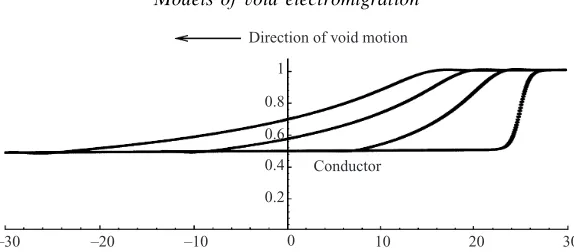
suggests that for a long thin conductor subjected to a uniform electric field at its ends, a void at the conductor boundary will undergo fairly steady translation for a time, with a steepening profile, until some critical void shape is attained. At this point the void motion becomes visibly unstable; a narrow finger emerges from the void and propagates transversely to the electric field until it has traversed the conductor height, and circuit failure occurs [1]. Damage of this kind can be suppressed by covering the exposed surfaces of the conductor with a layer of glass (‘passivating’) but in this case approximately-circular voids nucleate in the interior of the conductor, and these can again deform and cause failure. Both geometries (voids at a conductor boundary, and voids in the interior of a conductor) are therefore of interest.
Most of the existing literature on this problem is either experimental [1], numerical simulations [2, 24, 25, 32], or concerned with circular or nearly-circular voids translating in infinite conducting media [17]. The only exact solutions which have been written down explicitly are (i) the uniformly translating circular void (fixed area) in the infinite domain, and (ii) a flat front parallel to the electric field [24], which models the situation at the edge of the conductor. Linear stability of (i) has been treated by several authors, e.g. [17, 32], and stability of (ii) by Schimschak & Krug [24]. Numerical treatment of the ‘narrow finger’ instability mentioned above has been carried out recently by several authors [11, 27, 18, 19] (this problem has also been considered briefly in Suoet al. [30]). However, recent numerical evidence [2] points to the existence of other exact travelling-wave solutions, in a strip geometry: finite-sized non-circular (though nearly so) voids, and an unbounded finger-shaped void (both symmetric about the strip centre-line) are found numerically, using a method similar to that used by McLean & Saffman [16] to solve the Hele-Shaw fingering problem.
the circular void is unstable in the absence of surface tension effects, while a ‘stagnation point’-type flat-front travelling wave can be either stable or unstable, depending on the direction of the current.
We also consider some possible solutions for static voids. In§6 we consider approximate solutions of the model, using methods of formal asymptotics. For a void at a conductor boundary (rather than in the interior of the metal), an approach similar to that used to describe surface waves on inviscid fluid of finite depth may be used. In the appropriate parameter r´egime we find that in the absence of surface tension effects, ‘long-wavelength’ voids are described by a first-order nonlinear wave equation, which can be solved semi-analytically, and whose solutions are steepening waveforms. Inclusion of the surface tension terms adds a fourth-order (diffusion-type) term to this equation, which must then be solved numerically. This work extends that of Schimschak & Krug [24], which considers only shallow voids at the conductor boundary. We present several solution types. Finally, we discuss the implications of our results and present our conclusions.
2 Mathematical model
We consider the standard two-dimensional model for the phenomenon, which is considered sufficient to describe most situations of interest. Conductors in real circuits tend to have dimensions length ∼ L (along the horizontal direction in Figure 1), depth ∼ D (into the paper in Figure 1), height ∼ h (in the vertical direction in figure 1) such that
L >> h >> D; Lis usually taken to be infinite, and so, sometimes, is h (the void in the unbounded geometry, which describes small voids in the interior of a conductor). The two dimensions we consider are in the (L, h)-plane, quantities being averaged over the
D-direction.
We denote the domain occupied by the metal by Ω(t), with boundary ∂Ω(t), oriented such thatΩlies to its left. In general,∂Ωis composed of fixed insulating portions∂cΩ, and the moving void boundaryΓ(t) (also assumed insulating, but with an additional kinematic boundary condition governing its motion). We shall usually suppress the time-dependence of the various functions, except where emphasis is needed. Our coordinate system (x, y) is here taken such that the applied electric field is parallel to thex-direction, and where we consider the strip geometry, the strip is parallel to the x-axis. The mathematical model for the electric potential φ(where the electric fieldE=−∇φ) within the conductor is:
∇2φ= 0 within Ω, (2.1)
∂φ
∂n = 0 on ∂Ω=∂cΩ∪Γ , (2.2)
−vn=−Z∗eM∂ 2φ
∂s2 +Mωγ ∂2κ
∂s2 onΓ , (2.3)
φx∼E∞ asx→+∞, (2.4)
φx∼const. asx→ −∞, (2.5)
Γ(0) specified, (2.6)
Figure 2. The conventions adopted in the model (2.1)–(2.3).
conventions adopted are indicated in Figure 2. In the above,vn is the velocity of Γ in the direction of n, Z∗e is the effective charge of a metal ion, M is the adatom mobility, ω is the atomic volume, γis the coefficient of surface tension, and κ is the curvature of
Γ, taken to be positive for a void of convex shape ( e.g. a circle). All of the physical parameters are assumed to be constant in our model.
The far-field behaviour specified in (2.4) assumes a uniform electric field E =−E∞i applied at infinity, the case we shall usually consider in this paper (though different behaviour can also be envisaged; for example in the local problems near the tip of a void, or describing the field at the junction of two or more conductors (see§4.2)). The value of the constant in (2.5) depends upon the geometry assumed at minus infinity; it must be consistent with current conservation. The effective chargeZ∗eof a metal ion can be either
positive or negative, due to the fact that there are two competing forces acting on the ions: the direct electrostatic interaction, which pushes the positively-charged ions towards the cathode, and the so-called ‘electron wind’ force, due to collisions of the electrons (which are moving towards the anode) with the ions. Each of these effects produces a force on the ions proportional to the applied electric field, hence the two effects can be combined as a single effective force on the ion, equal to the electric field strength multiplied by the ‘effective charge’ of the ion. In most common conductors (e.g. aluminium) the electron wind force dominates, and the value ofZ∗eis negative; we shall assume this in our model.
Physically the first term on the right-hand side of (2.3) represents surface diffusion of atoms under the influence of the electric field, in the direction of the electron flow when
Z∗e <0. In this case, the void moves in the direction opposite to the electron flow, that
is, in the sense of the electric field. The second term on the right-hand side of (2.3) is less obvious, but acts to minimise the surface energy G,
G= Z
Γγ ds=γ×length(Γ),
a discussion of general laws of diffusive surface motion). For voids of finite area, the constant area constraint is equivalent to the condition that there is to be no net creation or destruction of metal; without this constraint one would just get the kinematic boundary condition −vn =−Z∗eMφss−γκ. If Γ extends to infinity, and the void area is infinite, the condition still ensures conservation of metal mass, which is clearly always desirable on physical grounds. Note that without loss of generality we may takeZ∗e <0, since if it
is positive we can just replace φ by−φ, and work with−Z∗e <0. We may also assume E∞ >0 by a similar argument, for if not we can replacexby−xand solve the problem for −E∞. In any case, the signs of these parameters only influence which way the voids move within the conductor; with our conventions they move from right to left (this can be seen most clearly from the direct analysis of§6).
Before proceeding further, we nondimensionalise the problem, following Ben Amar [2]. We have four relevant dimensional physical parameters: Z∗e, M, γ and E∞ whose
dimensions are given in Appendix A; suppose also that l and τ are typical length- and time-scales (to be determined). If surface tension effects are dominant in the problem, l
must be given by l =E∞|Z∗e|/γ, since this combination of parameters is the only one
having the dimensions of length. Otherwise,lis determined by the geometry; for instance, if the void size is comparable to the conductor width 2h, we takel=h. In either case, the characteristic timescale is then given by τ=l2/(E
∞|Z∗e|M). Thus we scale x andy with l, time withτ,φwithE∞l,1 which results in the dimensionless model:
∇2φ= 0 within Ω, (2.7)
∂φ
∂n = 0 on ∂Ω= ˆ∂Ω∪Γ , (2.8)
−vn=∂ 2φ ∂s2 +σ
∂2κ
∂s2 onΓ , (2.9)
φ∼x as x→+∞, (2.10)
where the dimensionless parameter σ is given by
σ= E∞|ωγZ∗e|l2, (2.11)
and measures the relative effects of surface diffusion due to the surface tension, and that due to the electric field. For problems with σ 1 we may expect the void motion to be approximated by the (much simpler) Zero Surface Tension (ZST) model, with σ= 0. (Note that the ZST problem is time-reversible if we also change the sign of φ. Thus, given any ZST solution, there is an equivalent solution with the electric field and the free boundary motion both reversed.)
3 Complex variable formulation
Since we have a two-dimensional Laplacian moving boundary problem we may consider a complex variable approach; such methods have proved invaluable in studying similar problems such as classical Hele-Shaw flow [14]. Thus we set z=x+iy and introduce a complex electrical potentialw(z) =φ(x, y) +iψ(x, y), whereψis a harmonic conjugate of
φ.2We note here that a complex variable approach, consideringwas an analytic function ofz, has recently been considered by Bradleyet al.[3] for an electromigration problem in a strip. However, the situation there is different to that we consider, in that the current is applied across the width of the strip rather than along its length (the sides y=±1 of the conducting strip are taken to be equipotentials). They consider a slit-shaped void along the length of the strip. In this case, the problem reduces to a simple Hele-Shaw crack problem which can be solved explicitly – the electric potentialφin their solution is easily checked to be equivalent to the streamfunction for the zero-width (λ= 0) Saffman-Taylor finger solution [23]. This same approach was used earlier by Sornette & Vanneste [28, 29], on an equivalent problem in rupture in thermal fuse networks. Our aim is to formulate a more general complex variable approach.
An important concept we shall need is that of theSchwarz functionof an analytic curve
Γ(t): this is the unique complex functiong(z, t), analytic in some neighbourhood ofΓ(t), such that the equation ¯z=g(z, t) describes the curve. We remark at the outset that there are severe restrictions on a general complex functiong if it is to be a Schwarz function. On the curve we require
z=g(z) = ¯g(¯z) = ¯g(g(z)) = (¯g◦g)(z),
where ¯g is the complex conjugate function ofg, defined by ¯g(z) =g(¯z). Both sides of this equality are functions analytic in some neighbourhood of the curve, so the equality may be deduced to hold everywhere, by complex analytic continuation. Hence, ifgis to be the Schwarz function of an analytic curve, we require ¯g to be its inverse.
It can be shown [6] that geometrical properties of the curve may be simply expressed in terms of g; with the direction conventions established in Figure 2, and with prime denoting ∂/∂zwe have
vn=2√g−0(iz, t)∂∂gt(z, t), κ=i∂∂z
1 √
g0(z, t)
, ∂∂zs =√ 1
g0(z, t),
thus on Γ, ∂/∂s = (∂/∂z)/√g0(z, t). (The above expressions are readily verified for the
simple example of a circle of radius √t, for which g(z, t) =t/z.) On the void boundary
Γ(t), (2.8) implies that
∂2φ ∂s2 =
∂2w ∂s2.
Putting all this together, we can express the boundary condition (2.9) holding on Γ in complex variable form as:
i
2 ∂g
∂t =
∂ ∂z
1 √
g0(z)
∂ ∂z
w(z) +iσ∂∂z
1 √
g0(z)
. (3.1)
Sincewis analytic throughoutΩ(except at infinity), andgis known to be analytic at least in some neighbourhood of the void boundary Γ (assumed to be an analytic curve), this relation may be analytically continued [4] away from Γ, and deduced to hold wherever the various quantities are defined.
If the asymptotic behaviour is as in (2.10),w has the behaviour
w(z)∼z as<(z)→+∞. (3.2) Thus, without the added complication of fixed insulating boundaries to be dealt with (i.e. in the unbounded geometry) one may seek solutions for a given shape of void by: (i) finding the Schwarz function g of the postulated void shape (e.g. circle, ellipse, parabola,. . . ), and (ii) attempting to match the behaviour at infinity and eliminate any other singular behaviour of w within Ω in equation (3.1). If one wishes to consider solutions in a strip geometry −16y61 using this approach, one has to use aperiodic arrayof voids, so that the insulating conditions ony=±1 are satisfied automatically.
3.1 Conformal mapping
Another approach which can be helpful is to introduce a time-dependent conformal map
z=f(ζ, t) from some canonical domain in an auxiliary complexζ-plane, ontoΩ. Often in the following we shall drop the explicit time-dependence, writing f(ζ). The two simplest cases to envisage are (i) a finite void translating in an unbounded metal domain, and (ii) a semi-infinite void moving through a semi-infinite metal domain, though periodic generalisations of each of these cases (corresponding to a finite or infinite void (e.g. finger) in a conducting strip) are also feasible. In case (i) the most appropriate canonical domain to map from is the unit disc, withζ= 0 mapping to infinity such that
f(ζ)∼aζ as ζ→0;
in case (ii) it is the right-half plane, with asymptotic behaviour
F(ζ)∼Aζ asζ→ ∞ for a void boundary which is asymptotically flat, or
F(ζ)∼Aζ2 asζ→ ∞
for a void boundary which is asymptotically parabolic, etc. We now consider each case separately.
3.1.1 Mapping from the unit disc
Consider a time-dependent conformal map from the unit disc in an auxiliary complex
ζ-plane onto the metal domain Ω(t) ⊂ C, z = f(ζ, t). This is always possible by the Riemann mapping theorem; moreover if one insists that the origin ζ= 0 map to infinity in the z-plane, and that the negative real axis near ζ= 0 correspond to the positive real axis near z=∞, then the mapping is unique [4]. The free (void) boundary is then the image under f of|ζ|= 1, so on the boundary we have
g(z) = ¯z=f(ζ) = ¯f(¯ζ) = ¯f(1/ζ);
since the functions on the extreme left- and right-hand sides of this equality are analytic in some neighbourhood of the boundary, the equality
holds globally by analytic continuation. Using this and the relations ∂
∂z =
1
f0(ζ)
∂ ∂ζ,
∂ζ
∂t =− ft(ζ)
f0(ζ),
where the prime denotes∂/∂ζand the subscripttdenotes∂/∂t, we can thus reformulate equation (3.1) as a functional differential equation in the ζ-plane:
1
ζ2ft(ζ)¯f0(1/ζ) + ¯ft(1/ζ)f0(ζ) =−2 ∂ ∂ζ
ζW0(ζ)
(f0(ζ)¯f0(1/ζ))1/2
−2σ∂∂ζ (
ζ
(f0(ζ)¯f0(1/ζ))1/2 ∂ ∂ζ
" 1
f0(ζ)
∂ ∂ζ ζ
f0(ζ)
¯
f0(1/ζ)
1/2!#)
. (3.4)
Care is needed when choosing the branches of the square-roots on the right-hand side of (3.4). Here,W(ζ)≡w(f(ζ)) is the complex potential in theζ-plane, which may be written down explicitly for a given problem. For example, if we have a finite void translating within an unbounded domain, then forf to map conformally ontoΩfor|z| 1 we must have the behaviour f(ζ)∼a/ζ as ζ →0, for some constant a >0. From (3.2) and (2.8)
W thus satisfies
W(ζ)∼ a
ζ asζ→0, =(W) = 0 on|ζ|= 1,
and hence
W(ζ) =a
ζ+1ζ
. (3.5)
3.1.2 Mapping from a half-plane
Here we write the map as z=F(ζ, t) to distinguish from the unit disc case. If we write
ζ =ξ+iςthen the void boundary is given byz=F(iς),ς∈R, so on the boundary we have:
g(z) = ¯z=F(ζ) = ¯F(¯ζ) = ¯F(−ζ).
Thus reasoning as for the unit disc we deduce that
g(z) = ¯F(−ζ),
and we can again reformulate equation (3.1) as a functional differential equation holding in the ζ-plane:
Ft(ζ)¯F0(−ζ) + ¯F
t(−ζ)F0(ζ) =−2∂∂ζ
W0(ζ)
(F0(ζ)¯F0(−ζ))1/2
−2σ∂∂ζ (
1 (F0(ζ)¯F0(−ζ))1/2
∂ ∂ζ
" 1
F0(ζ)
∂ ∂ζ
F0(ζ)
¯
F0(−ζ)
1/2!#)
. (3.6)
Again, because of the fixed domain in ζ-space, W(ζ) may be written down explicitly for a given problem, though it will depend upon the asymptotic behaviour of both wandF. Suppose we seek a solution with an asymptotically-flat boundary; then we must have
with (2.8) also to be satisfied) we then require
W(ζ)∼Aζ asζ→ ∞, =(W) = 0 on<(ζ) = 0,
and hence
W(ζ) =Aζ, (3.7)
where A=iB for someB∈R. (This indicates that the asymptotically-flat boundary lies parallel to the electric field, since the far-field behaviour of the map F isF(ζ)∼iBζ and we are mapping from the right-half ζ-plane; this is the case considered by Schimschak & Krug [24]). However, if we are interested in a flat-front type solution as describing the situation near the ‘nose’ of a translating void, then the appropriate far-field behaviour for
w is
w(z)∼z2 as |z| → ∞, (3.8)
(cfa stagnation-point flow in fluid dynamics). The solution forW is then given by
W(ζ) =A2ζ2, (3.9)
where nowA2 is required to be real if the boundary condition (2.8) is to hold.
For a solution where the void boundary is asymptotically parabolic, F(ζ) ∼A2ζ2 as
ζ→ ∞for some A. In this case, with w satisfying (3.2) (instead of (3.8)), the solution for
W is again given by (3.9), since this satisfies
w(z) =W(ζ) =A2ζ2 ∼F(ζ) =z, for|z| 1,|ζ| 1.
4 Exact solutions 4.1 Travelling-wave solutions
We now consider some simple travelling-wave solutions to the model using the complex variable approach. Consider first the travelling-wave version of (3.1). The Schwarz function
g(z, t) must be of the form
g(z, t) =−V t¯ +g0(z+V t),
whereg0is the Schwarz function for the shape of the free boundary in the travelling-wave frame. In this frame, with ˆz=z+V t(where possiblyV ∈C) and functional dependence only on ˆz, (3.1) becomes:
q g0
0(ˆz)( ¯Vzˆ−Vg0(ˆz)) + 2σ d 2
dzˆ2 1 p
g0
0(ˆz) !
= 2idw
dzˆ; (4.1)
the velocity of the travelling wave is (−<(V),−=(V)). Even in the ZST case, withσ= 0, solutions to this model are difficult to find, becausewis required to be analytic throughout
Ω, yet the square-root of g0
Figure 3. The geometry of the flat-front travelling-wave. The metal occupies the shaded region, and the arrows there indicate the direction of the electric field. The arrows in the void region indicate the direction of the free boundary motion.
4.1.1 Circular travelling-wave void
The Schwarz function for a circular void of radius a centred on the origin is just
g0(ˆz) =a2/zˆ, which in (4.1), with V assumed real (this is easily seen to be necessary to satisfy the asymptotic behaviour (3.2)), leads to
w(ˆz) = aV2
ˆ
z+azˆ2
. (4.2)
Thus if we are to have w(z)∼z at infinity the void must move from right to left with a velocity of 2/a. This solution was first presented by Ho [13].
4.1.2 Flat-front travelling-wave
The Schwarz function for the straight line my=x is just g(z) =z(m−i)/(m+i). Thus (4.1) gives the complex electric potential necessary for a solution as
w(ˆz) = zˆ42((mm2−+ 1)i)1/23/2(( ¯V +V)−im( ¯V−V)). (4.3)
It is easily checked from (4.1) that there is no travelling wave parabola, for which
g0(ˆz) = ˆz−4a+4a√(1−z/aˆ ); this would lead to an unphysical square-root singularity inw.
4.1.3 Stability analyses forσ= 0
In this section we consider the linear stability of the travelling wave solutions found above. We do this in the absence of surface tension effects, although both solutions are valid for arbitraryσ. The most appropriate forms of the governing equations for this purpose are (3.4) and (3.6) (withσ= 0). We do the circular void first, which, as mentioned in the Introduction, has been considered by Mahadevan & Bradley [17] and Wanget al. [32].
Settinga= 1 andV = 2 for convenience in (4.2), the basic solution is given by
f(ζ, t) =−2t+1ζ, W(ζ) =ζ+1ζ.
We seek a perturbation of the form
f(ζ, t) =−2t+1ζ+ν(ζ, t), (4.4)
for some function ν(ζ, t) analytic on the unit disc, which must be expressible as a convergent sum of the form
ν(ζ, t) =X∞ k=0
dk(t)ζk, (4.5)
on the unit disc (there can be nok=−1 term if the void is to conserve its area). Since the void boundary is the image of ζ=eiθ (θ∈(0,2π)), and the d
k(t) are complex, it is easy to see how the representation of (4.5) corresponds to a harmonic perturbation to the free boundary as considered in a conventional stability analysis: taking real and imaginary parts in x(θ, t) +iy(θ, t) =f(eiθ, t) gives
x(θ, t) =−2t+ cosθ+ ∞ X
k=0
<(dk(t)) cos(kθ)− =(dk(t)) sin(kθ),
y(θ, t) =−sinθ+X∞
k=0
<(dk(t)) sin(kθ) +=(dk(t)) cos(kθ).
The complex potential in the ζ-plane,W(ζ), must remain unchanged in order to satisfy the condition that its imaginary part vanish on |ζ|= 1 (but the potential in thez-plane,
w(z), must change as the solution is perturbed); this is why tackling the problem in the
ζ-plane is so appropriate. Substituting for W and the perturbed f in (3.4) the leading orders match automatically (on choosing the appropriate sign for the square-root on the right-hand side of (3.4)), and equating the terms of order on both sides yields two equations forν:
∂ ∂ζ
ζ(ζ2−1)∂ν ∂ζ
+ 2∂∂νζ+∂∂νt = 0, (4.6)
and solving the resulting eigenvalue problem forµ. This is difficult here due to the form of the differential operator in (4.6), hence we adopt the following non-standard approach. Direct substitution of (4.5) in (4.6) yields
O(1) : d1+ ˙d0= 0,
O(ζ) : d˙1= 0,
O(ζk) : (k2−1)(d
k−1−dk+1) + ˙dk= 0, k>2. The first two equations can clearly be solved immediately, giving
d1(t) =d1(0), d0(t) =d0(0)−d1(0)t,
and we may decouple these modes from the remainder of the terms by defining
D2m+1(t) :=d2m+1(t)−d1(0), D2m(t) :=d2m(t),
form>1. Then the function
N(ζ, t) =
∞ X
k=2
Dk(t)ζk≡X∞ k=2
dk(t)ζk−d1(0)ζ3
1−ζ2 , (4.7)
satisfies the same equation (4.6), for|ζ|<1. Note that|ζ|= 1 is the circle of convergence forN(ζ, t); asζ→1 we have the local behaviour
N(ζ, t)∼ −2(1d1(0)−ζ)+O(1), (4.8)
since the sumP∞k=2dk(t)ζkis assumed convergent on the unit disc. We may write equation (4.6) forN in self-adjoint form as
∂ ∂ζ
(ζ2−1)2
ζ
∂N
∂ζ
+(ζ2ζ−2 1)∂∂Nt = 0, (4.9)
valid for|ζ|<1 (the singularity atζ= 0 is removeable with the form forN(ζ, t) in (4.7)). We now restrict attention to the interval (0,1) of the real axis (where (4.9) must certainly hold, since it holds on the entire unit disc) and make the substitution ζ=e−x, x∈(0,∞). WritingN(x, t) =N(ζ, t) on this interval gives the equation for Nas
2∂∂x
∂N ∂x sinh2x
=∂N∂t sinhx,
and finally, writingB(x, t) =N(x, t) sinhx gives ∂B
∂t = 2 sinhx
∂2B ∂x2 −B
. (4.10)
The boundary conditions on B(x) are imposed atx= 0 (ζ= 1) andx=∞(ζ= 0). Since by (4.8) N(x, t)∼ −d1(0)/(2x) as x→0, we have B(0, t) =−d1(0)/2, and since by (4.7)
N(ζ, t)∼D2(t)ζ2 asζ→0,N(x, t)∼D2(t)e−2xas x→ ∞, and so B(x, t)→0 as x→ ∞. Thus we have to solve the diffusion equation (4.10) subject to these boundary conditions:
and an initial condition, which is readily verified to be
B(x,0) =X∞ k=2
dk(0)e−kxsinhx−d1(0) 2 e−2x.
As remarked, (4.10) is a diffusion equation on (0,∞), with positive diffusion coefficient sinhx. Thus ast→ ∞ we expect thatB(x, t) tends to the steady-state solution satisfying both boundary conditions, namely
B(x,∞) =−d12(0)e−x.
Defining ˆB(x, t) = B(x, t) +d1(0)e−x/2, ˆB satisfies (4.10) plus homogeneous boundary conditions ˆB(0, t) = 0 = ˆB(∞, t). Multiplying equation (4.10) for ˆB through by ˆB and integrating between x= 0 andx=∞, using these boundary conditions, we find
1 2
d dt
Z ∞
0 ˆ
B2
sinhxdx=−2 Z ∞
0 ( ˆB 2
x+ ˆB2)dx <0.
This reveals ˆB to be decreasing in time, implying that B does approach the steady-state solution ast→ ∞. Thus
N(x, t)→ −dex1(0)−ee−−xx,
⇒N(ζ, t)→ −d11(0)−ζζ22 =−d1(0)
∞ X
k=1
ζ2k. (4.11)
Here, (4.11) holds not only on the real interval 0< ζ <1, but on the entire open unit disc |ζ|<1. This is because the functionN(ζ, t) is known to be complex analytic on|ζ|<1, thus if it is known on a dense subset of the unit disc (the interval 0 <<(ζ)<1), this result can be analytically continued [4] to the whole unit disc. It follows that
D2k → −d1(0), D2k+1→0 (k>1), as t→ ∞, and
dk(t)→(−1)k+1d1(0) k>2,
as t → ∞. Thus the sum (4.5) representing the perturbation to the circular boundary slowly becomes divergent as tincreases, since
ν(ζ, t)∼(d0(0)−d1(0)t)−d1(0)
∞ X
k=1
(−1)kζk, t1
= (d0(0)−d1(0)t) +d1 +1(0)ζζ,
forward-most point (the image ofζ=−1). The fact that the coefficient d1(0) is arbitrary and complex corresponds to the fact that the protruberance/dimple may start to grow in any direction from this point. In the ‘spike’ limit, the angle made by the spike with the axis of translation is tan−1(=(d1(0))/<(d1(0)))), hence we expect this to be the initial direction of growth. Both scenarios have been observed in numerical simulations on circular voids; protruberances in Mahadevan & Bradley [17] and Schimschak & Krug [25], and dimples in Li et al. [15] and Schimschak & Krug [25]. Both cases are of interest: in the former case, the growth direction is arbitrary, hence the instability may mark the onset of a finger-shaped void propagating at an angle to the electric field such as those observed in experiments [1] and simulations [18, 19] of conductor failure. In the latter case, a dimple pointing into the void may herald the onset of void break-up via so-called ‘invagination’, which has been observed in the simulations of Liet al. [15] and Schimschak & Krug [25]. Now consider the simple flat-front solutions, for which the stability analysis is more straightforward. The solution of Figure 3 is given in the notation of (3.6) by F(ζ, t) = −2t+ζ, W(ζ) =ζ2; again we have normalised so that we have a wave of speed 2. We perturb this solution, writing
F(ζ, t) =−2t+ζ+ν(ζ, t).
Substituting in (3.6), the leading-order terms match automatically, and equating theO() terms gives
∂ ∂ζ
ζ2∂ν
∂ζ
−ζ2∂∂νt = 0, (4.12)
(plus an equivalent equation for ¯ν(−ζ, t)) after recasting in self-adjoint form. This equation holds for all<(ζ)>0. We now restrict attention to the positiveξ-axis (ζ=ξ+iς), writing
ξν(ξ) =B(ξ) there;B then satisfies the diffusion-type equation ∂B
∂t = 2ξ
∂2B
∂ξ2, ξ>0. (4.13)
For the stability analysis we seek a perturbation νsuch that on the boundary
ν(iς, t) =X∞ k=1
dk(t)e−ikς=
∞ X
k=1
dk(t)e−kζξ=0
(we need the minus sign in the exponent forν to represent an acceptable perturbation toF as <(ζ)→ ∞; as with the circular void, this can be seen to represent a harmonic perturbation to the free boundary). Thusν(ξ) is at most order e−ξ as ξ → ∞, implying thatB(ξ) =O(ξe−ξ) asξ→ ∞, soB(∞) = 0. Also, we must have|ν(0)|<∞, so B(0) = 0 also, and we have two homogeneous boundary conditions on B.
Assuming a time-dependence of the form B(ξ, t) =eµtB˜(ξ), we multiply (4.13) by ˜B(ξ) and integrate between zero and infinity, giving
− Z ∞
0 (˜B
0(ξ)2)dξ=µ 2
Z ∞
0 ˜
B(ξ)2
ξ dξ; (4.14)
The reversed flat-front solution (Figure 3 with all arrows reversed) is given in the notation of (3.6) by F(ζ, t) = 2t+ζ, W(ζ) = −ζ2. Exactly the same procedure reveals (4.12) and (4.13) to be replaced by
∂ ∂ζ
ζ2∂ν
∂ζ
+ζ2∂∂νt = 0, −∂∂Bt = 2ξ∂∂2ξB2, ξ>0 (4.15)
respectively, thus in (4.14) the sign of µis reversed, and this flat front travelling wave is linearly unstable.
With these two results together, we could have predicted the result for the circular void, since they imply that the rear of the circular void ought to be stable, while the front should be unstable, exactly as we found. We note that the stability of the circular travelling wave when σ0 was considered numerically for the full problem by [17, 32] and it was found to be stable for all values of σ treated. The linear stability for σ >0, and the nonlinear stability forσ >0, remain as interesting unresolved issues.
4.1.4 The circular void is the only travelling wave void of finite area in the unbounded geometry
We can in fact prove that the only travelling wave void solution (subject to the asymptotic behaviour (3.2)) having finite void area in an unbounded metal domain is the circular solution of § 4.1.1. The proof uses the formulation of equation (4.1) as well as the conformal mapping ideas introduced in §3.1, and relies on a theorem due to Millar [20] (and in part due to Shapiro [26]). The theorem states that for a simple closed analytic curve Γ, whose Schwarz functiong is analytic outsideΓ and has behaviourg =O(|z|N) as |z| → ∞, the following holds: (i) if N∈ {−2,−3,−4, . . .}then no admissible Γ exists; (ii) if N =−1 then Γ is a circle centred on the origin; (iii) if N = 0 then Γ is a circle with centre displaced from the origin, and; (iv) ifN= 1 thenΓ is an ellipse with nonzero eccentricity.
We observe that the right-hand side of (4.1) is analytic throughout the metal domain
Ω, and approaches the constant value 2i at infinity. Hence the left-hand side must also represent a function analytic onΩwith this far field behaviour. We claim that this means
g0(ˆz) is necessarily analytic on the metal domain Ω ⊂ C (except possibly at infinity), so that Millar and Shapiro’s theorem is applicable. Once this claim is proved, the result follows quickly, as it is easily seen that the only possible large-|ˆz|behaviour ofg0 in (4.1) compatible with (3.2) is
g0(ˆz)∼ V¯42zˆ as|ˆz| → ∞. (4.16)
Thus, we have case (ii) of the theorem, and we conclude that the void boundary must be a circle centred on the origin, proving the result.
We now prove the claim that g0(ˆz) must be analytic on the metal domain Ω if (4.1) holds. This is done in several stages. First, we note that zeros of g0
0(ˆz) withinΩ are not allowed, except at infinity where the behaviour is found from (4.16). For, if g0
0(ˆz) vanishes at some point, then pg0
0(ˆz)( ¯V z−Vg0(ˆz)) = 0 on the left-hand side of (4.1), while the remaining term 2σ(d2/dzˆ2)(1/pg0
0(ˆz)) is unbounded, giving a singularity ofdw/dzˆ at that point, hence a contradiction. Sog0
In terms of the conformal mapping from the unit disc onto the domain Ω, g0
0(ˆz) may be represented as a function of ζ(see (3.3)):
g0
0(ˆz) =− ¯
f0(1/ζ)
ζ2f0(ζ). (4.17)
It follows that ¯f0(1/ζ) cannot vanish on |ζ| 6 1 except at ζ = 0 (which maps to the
point at infinity in Ω), and therefore thatf0(ζ) cannot vanish on |ζ|>1 except atζ=∞.
By conformality, f0(ζ)0 on |ζ|61, and we conclude that f0(ζ)0 for 0 6|ζ|<∞.
Likewise, ¯f0(1/ζ)0 for 0<|ζ|6∞. From (4.17) then,g0
0(ˆz) is bounded and nonzero (as a function of ζ) on the unit disc, except at ζ= 0; hence it is bounded and nonzero (as a function of ˆz) onΩ except at ˆz=∞, where the behaviour is given by (4.16). Sog0
0(ˆz) is bounded on Ω, and nonzero except at infinity.
It follows thatg0
0(ˆz) can only have certain types of branch-point singularities inΩ(things like poles would obviously give infinities). Suppose there is a singularity at ˆz = ˆz0 ∈Ω; we write
g0
0(ˆz) =g00(ˆz0) +S0(ˆz) +· · · near ˆz= ˆz0, where g0
0(ˆz0)0, and S0(ˆz)→0 as ˆz→zˆ0.S0(ˆz) represents the local singular behaviour, which could be something likeS0(ˆz)∼√zˆ−zˆ
0, orS0(ˆz)∼(ˆz−zˆ0) log(ˆz−zˆ0), for example. Substituting this behaviour into (4.1) we find
g0(ˆz0)1/2+ S0(ˆz)
2g0(ˆz0)1/2 +· · ·
z0 V¯ −Vg0(ˆz0)−V S(ˆz) +· · ·−
σ
g0(ˆz0)3/2S000(ˆz) = (regular). Absorbing the regular parts into the right-hand side we require
−Vg0(ˆz
0)1/2S(ˆz) + zˆ0S
0(ˆz)
2g0(ˆz0)1/2 V¯ −Vg0(ˆz0)
−V S(ˆz)S0(ˆz) 2g0(ˆz0)1/2 −
σS000(ˆz)
g0(ˆz0)3/2 ≈0, (4.18) near ˆz= ˆz0. Considering the different possible leading-order balances in (4.18), it is clear that S000 balancing S0 and S leads to trivial nonsingular solutions. In any case, S000 must
be more singular than eitherS orS0, ifS is itself singular at ˆz
0. So suppose
V S(ˆz)S0(ˆz) +2σS000(ˆz) g0(ˆz0) ≈0.
This may be integrated twice, giving
σS0(ˆz)2
g0(ˆz0) + V S(ˆz)3
6 ≈k1S(ˆz) +k2,
for arbitraryk1andk2. The only possible singular behaviour of solutions to this equation is easily checked to beS(ˆz) =O(ˆz−zˆ0)−2, but since this represents an unbounded singularity in g0(ˆz), it is not allowable.
We conclude that there are no allowable singularities ofg0(ˆz) withinΩ, henceg0(ˆz), and
void. However, they do not work when V = 0 (static solutions), in which case there are non-circular solutions: see §4.2 below.
Taken together with the linear stability of the NZST travelling-wave circle problem (claimed from the numerical results of Mahadevan & Bradley [17] and Wanget al. [32]), this is an important result, as it suggests that for sufficiently large values of the surface tension parameterσ, a small void moving within a conductor will approach this travelling-wave circular form. As remarked in § 4.1.3 though, since the ZST problem is linearly unstable we expect the threshold perturbation (below which perturbations will decay, but above which they may grow) to tend to zero as σ→0. Thus for small values of σ, instabilities may be manifested, and this travelling-wave form may not be approached.
We note here that if the assumption of a perfectly insulating void is relaxed, i.e. the electrical conductivity within the void is nonzero (though always less than that outside the void), then other travelling wave solutions may exist. The model in this case is more complicated, as Laplace’s equation must be solved inside the void as well as outside. Here the single boundary condition∂φ/∂n= 0 on∂Ωis replaced by two jump conditions:
[φ]∂Ω= 0,
%∂∂φn
∂Ω= 0,
where % represents the electrical conductivity inside or outside the void. The second of these conditions represents continuity of the current passing through the void boundary (no jump in J ·n), while the continuity ofφ follows from the fact that∇ ∧E ≡ −∂B/∂t
must be bounded at the void boundary. Wang et al. [32] consider the case in which
%void =%metal, so that the electric field is simply uniform throughout. In this case their numerical simulations indicate that an initially circular void can approach an egg-shaped travelling wave ([32], Figure 4).
4.2 Steady solutions
It is of interest to note that the steady model, with vn ≡0 in (2.3), is exactly the steady one-phase Hele-Shaw model with surface tension effects included at the free boundary, if the electric potentialφ is identified withp, the pressure in the fluid, the metal domain
Ω with the domain occupied by fluid, and the void with an air-bubble in the cell. In the time-dependent Hele-Shaw problem,pis harmonic within the fluid domainΩ, and satisfies the kinematic boundary condition ∂p/∂n = −vn, and the dynamic boundary condition
p=−σκ, using the same notation as our formulation (2.7)–(2.9). Thus if one considers the steady case of each problem, with vn = 0, the Hele-Shaw kinematic boundary condition is equivalent to the ‘insulating void’ condition (2.8), and the electromigration kinematic boundary condition (2.9) may be integrated twice with respect to arclength s along the boundary:
φ=−σκ+k1s+k2. (4.19)
For single-valuedness of the potential,k1must be zero, and the arbitrary constantk2may be absorbed intoφ, so can be taken to be zero without loss of generality. Hence (4.19) is equivalent to the Hele-Shaw dynamic boundary condition.
Figure 4. The local situation at the junction of two conductors.
discovered by Entovet al.[8], with appropriate behaviour at infinity; it follows that these are also solutions to our model, provided w(z) has the correct behaviour at infinity. In the Hele-Shaw context, the solutions of Entovet al.[8] involve a bubble symmetric about bothx- andy-axes, with the complex potential F(z) (p=<(F)) having the behaviour
F(z) = 2πmzn+{analytic part} as|z| → ∞, (4.20) where m > 0 measures the strength of the ‘multipole singularity’ at infinity. For our problem F ≡ w, so the complex electric potential has the behaviour (4.20) at infinity. The casen = 1, which is our usual far-field condition, has no solution, but valuesn >1 give nontrivial equilibrium shapes. Consider for example the case n = 2. This far-field behaviour corresponds to an electric field aligned along hyperbolae at infinity, since the ‘streamfunction’ψ(the harmonic conjugate ofφhas behaviourψ∼mxy/πforx2+y2 1. Such behaviour may be appropriate to describe the local situation at a junction of two conductors, where current is flowing as indicated in Figure 4.
For each value of n>2 it is found that, depending on the value of the dimensionless parameter µ = (2πσ(n+ 1)/m)−2/(n+1)S/π (where S is the cross-sectional area of the bubble/void), there are either two, one or no solutions to the problem. More precisely, forµ < µ∗(n) (sufficiently small voids) there are two solutions; forµ=µ∗(n) there is one
solution (critical void size), and forµ > µ∗(n) there are no solutions. The values of µ∗(n)
5 The strip geometry: Voids in the interior
Ideally, we would like to be able to find some exact (travelling-wave or otherwise) solutions in the strip geometry, such as those found numerically for the ZST problem by Ben Amar [2] (infinite fingers, and finite rounded voids, both symmetric travelling-wave shapes). However, this appears far from simple, and we have been unsuccessful so far. As noted in § 3, to deal with the insulating conductor boundaries one has to consider a periodic array of voids. Suppose we wish to use the conformal mapping technique embodied in (3.6) to find an infinite symmetric ‘finger’ travelling wave solution. If we map from the right-half plane via z=F(ζ), the map must be periodic in the y-direction, generating an infinite array of identical fingers, so in theζ-plane the insulating walls must be the image of lines =(ζ) = constant; see Figure 5. Consideration of the map far ahead of the fingers (<(z) →+∞, <(ζ)→+∞) shows that F(ζ) ∼ζ there (or some constant multiple). Thus the complex potentialW(ζ) in the right-halfζ-plane must satisfyW(ζ)∼ζ
as <(ζ)→+∞, and have constant imaginary part on those lines=(ζ) = constant which correspond to the insulating walls. It follows that for a symmetric finger
W(ζ) = 2πlog(cosh(πζ/2)), (5.1) since this is periodic with =(W) = ±1 on the lines =(ζ) = ±1 (which correspond to the insulating sides of the strip), and has zero imaginary part on <(ζ) = 0 (which gives the void boundary). Also, (5.1) has the correct far-field behaviour as <(ζ)→+∞. Thus, neglecting surface tension effects, (3.6) reduces to the problem of finding the appropriate conformal map F(ζ, t) satisfying
Ft(ζ)¯F0(−ζ) + ¯Ft(−ζ)F0(ζ) =−2∂∂ζ
tanh(πζ/2) (F0(ζ)¯F0(−ζ))1/2
(5.2)
together with the appropriate behaviour far ahead of, far behind, and at the tip of, the finger. If one assumes a travelling-wave form for F, F(ζ, t) = b(t) +F0(ζ), one can integrate (5.2) (the constant of integration has to be zero from considerations at the finger-tipz=b(t) whereF0 has the local behaviourF0(ζ)∼ −ζ(π/(2˙b))1/2) giving
F0(ζ)−F¯0(−ζ) =−2˙b(F0tanh(πζ/2) 0(ζ)¯F00(−ζ))1/2
, (5.3)
but the problem is still formidable, and (other than the numerical evidence of Ben Amar [2]) we have no guarantee that a solution F0(ζ) satisfying all the requirements exists. The numerical finger solution appears to be uniquely selected, with a calculated width of 0.666 times the channel width, suggesting that the true widthλis 2/3. Even this unique selection is still a puzzle, as asymptotic analysis far behind the finger-tip gives only the single relation ˙bλ(1−λ) = −1, and it is not clear how to obtain a second relation. We remark that the finger-shape which solves the zero surface tension Hele-Shaw channel fingering problem [23] does not provide a solution to the electromigration problem, for any value of the finger width λ. Hele-Shawλ= 2/3 fingers are much blunter than those calculated in Ben Amar [2] for this problem.
Figure 5. The correspondence betweenz- andζ-planes for a finger-shaped void.
(and in fact we cannot hypothesise a simple periodic mapping in this case when the void is not enclosed by metal). We use asymptotic analysis to consider this situation in some detail in§6.
Being unable to find exact solutions in the strip geometry, we turn to approximate solutions, using methods from asymptotics.
5.1 Small voids in a strip
Throughout this subsection we neglect the effect of surface tension on the void shape and motion. Consider the simple case of a small, approximately circular void, radius
h, moving in a strip of width 2h, where 1. We assume the dimensionless model (2.7)–(2.10), where the lengthscale l used to nondimensionalise (as described in § 2) is taken to be h: the insulating boundaries are then at y = ±1, and the void has radius
. These dimensionless variables are the ‘outer’ variables, in which the void appears as a point singularity in the electric field, which, far from the singularity, isw(z)∼z.
the solution is a circular void of unit radius, exactly as given in §4.1.1:
˜
w0(˜z) = ˜
V
2
˜
z+1˜z
, ˜g0(˜z) = 1˜z, (5.4)
where ˜V is to be determined. This must match [31] onto the leading order outer solution as ˜z→ ∞. Writing (5.4) in terms of the outer variable we find
˜
w0(ˆz) = 2V˜
ˆ
z+zˆ2
, (5.5)
thus matching requires ˜V = 2, and the void travels with dimensionless speed 2 in the negativex-direction. The other piece of information we obtain from (5.5) is the nature of the singularity induced by the void in the outer solution. Together with the condition that =(w) be constant on the insulated walls y =±1 (ˆy =±1−β), this enables us to write down the next term in the outer solution:
w(ˆz) = ˆz+2π 4
cothπ
4zˆ
+ tanhπ
4(ˆz+ 2iβ)
+o(2) (5.6)
⇒ dwdzˆ = 1−2π2 16
cosech2π 4zˆ
−sech2π
4(ˆz+ 2iβ)
+o(2). (5.7)
To examine next order in the inner solution, we expand (5.7) near ˆz= 0, and write it in terms of the inner variables to see how the expansion for dw/d˜ ˜zproceeds, and what the large-˜zbehaviour must be. Using the fact that cosechx∼(1/x)−x/6 +O(x3) for smallx we see that (5.7) implies the large |˜z|behaviour
1
dw˜
d˜z = 1−
1 ˜
z2 +2 π2 16
1 3 + sec2
πβ
2
+O(3)≡1− 1 ˜
z2 +2λ+O(3) (5.8) (defining the real constantλ for convenience). Thus the next term in the expansion for ˜w
isO(3). The expansions in the inner proceed as:
˜
w=
˜
z+1˜z +2w˜
2+3w˜3+· · ·
,
˜
g =1˜z +2˜g
2+3g˜3+· · ·, ˜
V =(2 +2V˜
2+3V˜3+· · ·), where ˜w2 has the far-field behaviour (necessary for the matching)
˜
w0
2(˜z)∼λ, (5.9)
as |˜z| → ∞. Substituting these expansions into (4.1) (with V = ˜V, w = ˜w, g = ˜g, z= ˜z
andσ= 0), leading order matching is now automatic, and at first order we obtain
(˜z2−1)d˜g2
d˜z +
2 ˜
zg˜2=−2 dw˜2
d˜z + ¯˜V2−
˜
V2 ˜
z2. (5.10)
We require conservation of the area S of the perturbed void, which may be expressed as
S= Z Z
Voiddxdy= 1 2i
I ¯˜
z d˜z= 21i I
˜
g(˜z)d˜z=21i I
˜
g0(˜z)d˜z,
Hence we require
I ˜
gm(˜z)d˜z= 0, m >0. (5.11)
Using (5.10) and (5.9) we find the most general solution for the first order problem is
˜
w2(˜z) =λ
˜
z+1˜
z
+c˜2
z2, g˜2(˜z) =c2
1 +˜1
z2
, V˜2 = 2λ,
where c2 is an arbitrary constant. The void is still circular at this order, with at most an order2 shift in its centre along the direction of its motion; without loss of generality (by absorbing this shift into the leading order solution) we may takec2= 0 and so ˜g2(˜z)≡0. The only effect of the finite conductor width at this order is the real O(2) correction to its velocity provided by ˜V2: the void velocity in the (dimensionless) outer variables isV = 2+22λ. Any correction to the void shape comes in at a higher order. This is in agreement with the numerical results of Ben Amar [2], who found that voids translating in the interior of a conducting strip are very nearly circular in shape, even when relatively large.
6 The strip geometry: Voids at a conductor boundary
In this section we abandon our complex variable approach, and instead use asymptotic methods similar to those used in hydrodynamics to describe free-surface disturbances on water of finite depth (see e.g. [22] chapters 2 and 3 for a discussion). We return to the dimensional problem (2.1)–(2.4), writing A =−Z∗eM and B =Mωγ (both positive) for
convenience. The problem is shown in figure 6, with a void on the upper boundary which for the moment is assumed to be of infinite extent, and to be described by y =η(x, t), withη(∞, t) = 0 andη(−∞, t) =Q.
With this notation we have
vn= (1 +ηηt2
x)1/2, κ=
ηxx (1 +η2
x)3/2,
and the derivative with respect to arclength salong the free boundary is given by
∂s=(1 +1η2
x)1/2(∂x+ηx∂y),
thus the boundary conditions may be expressed in terms ofφandη. The full dimensional model is:
∇2φ= 0 −h
0< y < η, (6.1)
φy=ηxφx ony=η, (6.2)
−ηt=A(∂x+ηx∂y)
φx+ηxφy (1 +η2
x)1/2
+B∂∂x
1 (1 +η2
x)1/2 ∂ ∂x
ηxx (1 +η2
x)3/2
ony=η, (6.3)
φy= 0 on y=−h0, (6.4)
φx∼E∞, η∼0 as x→ ∞, (6.5)
φx∼hh0E∞
Figure 6. The full problem in the dimensional variables.
Suppose now that the initial profile is of the formη(x,0) =η0N(x/l), so thatl andη0 are lengthscales of the disturbance in thexandy directions, respectively. We then scale:
x=l¯x, y=h0¯y, η=η0η, t¯ =t0¯t, φ=φ0φ,¯
where t0 and φ0 are to be determined. It is natural to scale φ with the applied electric field at infinity; we thus choose φ0=E∞l. The appropriate time scaling is obtained from equation (6.3), and clearly depends upon which of the two terms on the right-hand side of this equation dominate. If the second term dominates we have, at least to leading order, motion of the free surface under surface tension subject to a volume constraint. Since this has been extensively studied elsewhere (see Elliott & Garcke [7] and the references therein), and is not really the subject of this work, we scale time with the first of the two terms by taking t0 =lη0/(AE∞). We thereby implicitly assume that effects due to the electric field either dominate, or are comparable with, surface tension effects. Before writing down the dimensionless model it is helpful to introduce the following two dimensionless parameters:
= ηh0 0 ∼
‘amplitude’
‘depth’ , δ=
h0
l ∼
‘depth’ ‘wavelength’,
(borrowing concepts from fluid dynamics rather loosely here). With these definitions the rescaling discussed above yields the following dimensionless model (dropping overbars for convenience):
δ2φ
xx+φyy= 0 −1< y < η, (6.7)
φy=δ2ηxφx ony=η, (6.8)
−ηt= (∂x+ηx∂y)
φx+ηxφy (1 +2δ2η2
x)1/2
+σ∗ ∂
∂x
1 (1 +2δ2η2
x)1/2 ∂ ∂x
ηxx (1 +2δ2η2
x)3/2
ony=η, (6.9)
φy= 0 ony=−1, (6.10)
φx∼ 1 +1Q∗, η∼ Q∗ asx→ −∞, (6.12)
where dimensionless coefficients Q∗ andσ∗ are defined as follows:
Q∗= Q
η0 σ
∗ = Bη0
Al3E∞ σ∗6O(1)
.
To get a simplified approximate model, we want to consider the case in which one or both of the parameters andδ are small. We now consider different cases.
The case δ 1, = 1
This is the case of a long-wavelength but deep void. Here we search for an asymptotic solution of the form
φ=φ(0)+δ2φ(1)+O(δ4), η =η(0)+δ2η(1)+O(δ4). Substitution of the above into equations (6.7)–(6.11) at leading order yields
φ(0)=φ(0)(x, t), (6.13)
η(0)t =φ(0)
xx−σ∗η(0)xxxx, (6.14)
φ(0)
x ∼1, η(0)∼0 asx→ ∞ (6.15)
φ(0)
x ∼ 1 +1Q∗, η(0)∼ Q∗ asx→ −∞, (6.16)
whilst at first order we find the following problem forφ(1):
φ(1)
yy+φ(0)xx = 0, (6.17)
φ(1)
y = 0 ony =−1, (6.18)
φ(1)
y =ηx(0)φ(0)x ony=−1. (6.19) Integrating equation (6.17) between y = −1 and y = η(0) and applying the boundary conditions (6.18) and (6.19) leads to the following relation:
∂
∂x φ(0)x 1 +η(0)
= 0, (6.20)
expressing conservation of electric current. We integrate this equation, apply the boundary conditions (6.15) and (6.16) and use the result to eliminate φ(0)
x from (6.14). Writing
f =η(0)+ 1 this leads to the following parabolic nonlinear PDE describing the evolution of the free surface:
ft+
1
f
x+σ
∗f
xxxx= 0, f(∞, t) = 1, f(−∞, t) =λ, (6.21)
where λ = 1 +Q∗. Thus, we have a model with just one dimensionless parameter σ∗, a
kind of dimensionless surface tension coefficient, which measures the relative effects of surface diffusion due to the surface tension and surface diffusion due to the electric field. A simple extension of this model is to consider a variable lower conductor boundary,