Abstract—Relays play important role in deployment of Long
Term Evolution (LTE) and LTE-Advanced systems. This paper addresses prediction of the radio signal path loss on the link between eNodeB and relay stations. The path loss models are derived on a basis of an extensive measurement campaign conducted in 1900 MHz frequency band. An effect of the relay station antenna height is studied and included in the path loss modeling. Good agreement between measurement and predictions is obtained, with standard deviation of the prediction error ranging between 2.59 and 6.34 dB.
Index Terms—LTE-Advanced, path loss measurements,
propagation model, relays, relay antenna height.
I. INTRODUCTION
URRUNT 3G systems are not capable of providing very high data rate to a large number of users. The Third Generation Partnership Project Long-Term Evolution (3GPP-LTE) and 3GPP-LTE-Advanced are developing technologies that meet ever increasing demand for higher data rate. LTE-Advanced is the upcoming global cellular technology that offers very high throughput on air interface. Table I summarizes important requirements for performance of the LTE-Advanced [1].
TABLEI
IMPORTANT LTE-ADVANCED PARAMETERS
Peak data rate (Gbps) DL 1 Antenna configuration UL 0.5
Peak spectrum efficiency (bps/Hz)
DL 30 (8x8)
UL 15 (4x4)
Average spectrum efficiency (bps/Hz/cell)
DL 2.4 2.6 3.7
(2x2) (4x2) (4x4)
UL 1.2 2.0 (1x2) (2x4)
Cell edge user throughput (bps/Hz/cell/user)
DL 0.07 0.09 0.12
(2x2) (4x2) (4x4)
UL 0.04 0.07
(1x2) (2x4)
Mobility up to 500 km/h
Bandwidth scalable bandwidth up to 100 MHz Modulation scheme QPSK, 16 QAM and 64 QAM
One of most promising technology that helps LTE-Advanced meet these requirements is the use of relays. Within LTE and LTE-Advanced, radio relays are used to extend coverage, enhance capacity, increase throughput and
Manuscript received June 21, 2013; revised July 12, 2013.
M. Hamid is a PhD candidate in the Electrical and Computer Engineering Department, Florida Institute of Technology, Melbourne, FL 32901 USA (phone: 321-960-6110; e-mail: [email protected]).
I. Kostanic is with the Electrical and Computer Engineering Department, Florida Institute of Technology, Melbourne, FL 32901 USA, (phone: 321-674-7189; e-mail: [email protected]).
provide overall increase in the network performance[2]-[4]. In addition to performance enhancements, the relays reduce cost of the network deployment and facilitate speed of the network roll-outs [5]. In many cases, relaying technique is considered as a viable solution for replacement of base stations. Relays cost significantly less than base stations. When deployed, relays act like base stations but without the need of wired connection to the backhaul.
From the network planning perspective one needs to be able to successfully model the impact of the relay deployment within an LTE network. The first step in this modeling is the prediction of the path loss on the link between the eNodeB and a relay station.
The measurement campaign discussed in this paper is set up specifically to evaluate the path loss encountered on eNodeB-relay link.
The review of literature shows that there is a general shortage of measured data collection to help empirical understanding of the propagation conditions in relay environment. Nevertheless, there have been several studies that discussed this topic.
Some of propagation models have been suggested by 3GPP (3rd Generation Partnership Project) [4], WINNER (Wireless World Initiative New Radio) [6] and IEEE 802.16j task group [7]. Nonetheless, one notes that a general limitation of these models is that they are developed from already existing propagation models that were derived under completely different assumptions. Hence their applicability to relay scenarios needs to be tested. Another limitation is that they were derived for certain levels of relay antenna height and therefore their validation for different heights still needs to be studied. In [8], the effect of receive antenna height on the received signal level in a LTE-Advanced relaying scenario was investigated. Even though general dependence of path loss on relay station antenna height was obtained, study would have been more complete if the authors had proposed an empirical path loss model which can be applied in similar scenarios. Similar to the work done in [8], authors in [9] proposed a new propagation model for relay scenarios; however, this model was suggested just for urban environments. Related work is to be found in [10]; however, the maximum height of relay station antenna was limited to 5 meters which is too low for most relay scenarios according to [4], [6].
The objective of this paper is to describe and document measurement campaign in relay environment, propose propagation models for eNodeB-relay link for multiple relay antenna heights and provide statistical analysis for the proposed empirical models. The outline of the paper is presented as follows. Section 2 discusses the setup used in the relay path loss measurement; empirical model derivation
Path Loss Measurements for Relay Stations in
1900MHz Band
Masoud Hamid and Ivica Kostanic
is discusses in Section 3; Section 4 presents the obtained measured data and some conclusions are drawn in Section 5.
II. MEASUREMENT SETUP
A. Equipment Description
The measurement system consists of a transmitter, transmit antenna, receiver, receive antenna, GPS (Global Positioning System) antenna and a laptop with installed measurement software from Grayson wireless. The software is used to measure the strength of the received signal and map its value on the spectrum tracker screen along with the corresponding frequency. Before measurements were conducted, spectrum clearing of the area was performed to verify that the frequency used for the path loss measurements is free from any sources of radiation.
B. Environment Description
The measurements conducted for this study are collected in a typical US suburban environment of Melbourne, FL, USA. Most houses in the selected area are single to double stories and their heights are about 4 to 9 meters. In general, most of the buildings are made of wooden structures with exception of few buildings that are made of combined materials; concrete for frame or body and timber or plastered bricks for walls, glass for windows, concrete for floors. Few buildings have flat roofs while most of one story houses and two stories residential apartments have pitched roofs. The terrain in general is flat with moderate tree densities. Trees height is up to 13 m.
C. Measurement Procedure Description
The measurements are collected in 1900MHz band which is one of the principal bands for the deployment of the LTE and LTE-Advanced. The parameters associated with the measurements are provided in Table II. As seen, the study is conducted using four different relay heights ranging from 4 to 16 m, which are typical heights where one would find relay deployment in various scenarios. The transmitter antenna (i.e. eNodeB antenna) is fixed to 25.5m.
For each examined relay antenna height, 124 of path loss measurement locations are examined. For each measurement location several hundred readings are averaged in time domain so that the fast-fading component of the signal is smoothed out. At each measurement point, GPS is used to determine the coordinates of the receiver. Consequently, the distance from the base station to the receiver can be
calculated. The location of the measurement points is presented in Fig. 1.
The transmitter is on the top of a multi-story building. The receiver is placed in a “boom-lift” as shown in Fig. 2 and moved between locations. The measurements are conducted over a period of couple of weeks, with essentially no changes in weather pattern and vegetation.
III. EMPIRICAL MODEL
In general, the measured path loss in [dB] between eNodeB and Relay Node (RN) is calculated by:
(1) where Pt is the transmitted power in [dBm], Gt is the
transmit antenna gain in [dB], CLt is the cable lose of the
transmitter in [dB], Pr is the received power in [dBm], Gr is
the receiving antenna gain in [dB] and CLr is the cable lose
at reception side in [dB].
TABLEII
PARAMETERS ASSOCIATED WITH THE MEASUREMENT CAMPAIGN
Parameter Value
Operating frequency 1925 MHz
T
ra
n
sm
it
te
r Antenna height 25.5 m
Transmitting power 43 dBm
Antenna gain 6 dBi
Cable and connector losses 0.7 dB
Re
c
e
iv
e
r Antenna height 4, 8, 12, 16 m
Antenna gain including cable
and connector losses 5 dBi
Noise figure 2 dB
[image:2.595.133.479.619.750.2]Fig. 2. Illustration of the transmitter (left) and the receiver (right)
A. Log Distance Path Loss Model
In the first order approximation, the predicted path loss in [dB] at any given distance d from the transmitter with respect to a reference distance d0 may be described as log-distance path loss model and given by:
(2) where represents the intercept in [dB] and m is the slope of the model in [dB/decade]. is a log normally distributed random variable that describes the shadowing effects. The parameters and m are environmentally dependent parameters and are usually determined through statistical analysis of path loss data measurements in a given environment.
B. Model Parameters Estimation Method
The task is to develop an empirical propagation path loss model that explains the observed data in the relay environment. MMSE (Minimum Mean Square Error) method was used to minimize the difference between prediction and measurements. Assuming that there are N measurements, the difference between measured and predicted path loss values for the ith point is expressed as:
(3)
where is the prediction error for the ith point and i=1,2, ... N. By substituting (2) into (3), one may write:
(4)
Taking all measurement points into account, the expression in (4) may be written in a matrix format as:
(5)
The approach here is to determine the optimum values of and m that minimize the norm of the vector δ. In other words, the cost function given by:
(6) needs to be minimized.
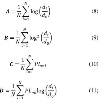
Substituting (6) into (5), taking the partial derivatives with respect to and m, and solving for the minimum yields:
(7)
where
(8)
(9)
(10)
(11) Therefore, the optimum values of and m can be given as:
(12)
(13)
IV. RESULTS AND DATA ANALYSIS
This section compares path loss measurements with path losses predicted using the model given in (2). The optimum values of and m were obtained according to the procedure explained in Section 3.
A. Performance Analysis of Path Loss Measurements The path loss measurements from which the antenna pattern effects have been taken out are presented in Fig. 3. Free space path loss is plotted as well and as it is seen, it represents a lower boundary for the measurements. One can easily observe that the measurements show consistent trends. The increase of path loss is a linear function of the log of distance. The figure shows clearly the effect of the relay antenna height on the path loss value in which these values decrease with the increase of relay antenna height. Measurements show less dependency of path loss value on the relay antenna height when the receiver is closer to the transmitter. This result may be explained by the fact that in such cases the receiver and the transmitter are in Line Of Sight (LOS) conditions in which relay antenna height does not have a significant impact on the received power. On the other hand, as the distance becomes larger, this dependency is more pronounced especially at lower relay antenna heights.
[image:3.595.376.550.54.227.2]Fig. 3. Measured and predicted path loss for different relay heights
TABLE III
RELAY PATH LOSS PROPAGATION MODEL PARAMETERS
Relay height [m] PL0 [dB] m [dB/dec.] σ [dB]
4 87.48 38.14 6.34
8 85.23 31.84 4.98
12 84.04 27.22 3.81
16 82.93 25.34 2.59
Free space 78.13 20 ---
Table III also shows the standard deviation (σ) of the prediction error between the predicted and measured path loss values.
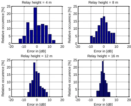
[image:4.595.61.278.277.353.2]Histograms in Fig. 4 describe the distribution of the prediction errors about their means for different relay antenna heights. It is observed that errors are almost log normally distributed about zero means with a standard deviation that decreases with the increase of the relay antenna height. The standard deviation, σ, ranges from 6.34 dB for lowest relay height to 2.59 dB for the highest one.
Fig. 4. Distribution of prediction error for the examined relay antenna heights
B. Path Loss Models at Different RN Antenna Heights According to (2) and Table III, one can write the propagation path loss model for any of the examined RN antenna heights. For example, in the case of 4 m relay, the model is given as:
(14) Similar to (14), other models for the corresponding relay antenna heights 8 m, 12 m, and 16 m can be expressed as well. These models are valid for 1900 MHz frequency band and d ranges from 100-4000 m.
It is of great interest to provide an empirical propagation path loss model that can be applied in relaying scenarios for different relay antenna heights in suburban environment. This model can be given as:
(15) whereas is the relay antenna height correction factor. In other words, represents the reduction of the path loss as the result of the relay antenna height increases. Fig. 5 illustrates distributions of the path loss differences for the examined relay antenna heights. Table IV shows these differences quantitatively in terms of their means and standard deviations. The smallest average reduction of path loss of 3.21 dB is obtained when the relay antenna height is changed from 12 to 16 m. Similarly, an average of 18.46 dB path loss difference is observed when the relay height is raised from 4 to 16 m.
Fig. 5. Distribution of path loss differences between different relay heights
TABLE IV
AVERAGE OF PATH LOSS DIFFERENCES BETWEEN RELAY HEIGHTS
Mean [dB] Standard deviation [dB]
PL(h=4) - PL(h=8) 9.08 6.05
PL(h=8) - PL(h=12) 6.16 4.22
PL(h=4) - PL(h=12) 15.25 7.55
PL(h=12) - PL(h=16) 3.21 3.59
PL(h=8) - PL(h=16) 9.38 5.26
PL(h=4) - PL(h=16) 18.46 8.27
C. Relay Antenna Height Correction Factor
According to Table IV, the average relay antenna height correction factor may be approximated as:
(16)
where h is the relay antenna height. Graphically, this
102 103
70 80 90 100 110 120 130 140 150 160 Distance [m] P a th L o s s [ d B ]
h=4 m - Measured h=4 m - Predicted h=8 m - Measured h=8 m - Predicted h=12 m - Measured h=12 m - Predicted h=16 m - Measured h=16 m - Predicted Free Space
-20 -10 0 10 20
0 5 10 15 20 25
Error in [dB]
R e la ti v e o c c u re n c e [ % ]
Relay height = 4 m
-20 -10 0 10 20
0 5 10 15 20 25
Error in [dB]
R e la ti v e o c c u re n c e [ % ]
Relay height = 8 m
-20 -10 0 10 20
0 5 10 15 20 25
Error in [dB]
R e la ti v e o c c u re n c e [ % ]
Relay height = 12 m
-20 -10 0 10 20
0 5 10 15 20 25
Error in [dB]
R e la ti v e o c c u re n c e [ % ]
Relay height = 16 m
-10 0 10 20 30
0 10 20
PL(h=4) - PL(h=8)
-10 0 10 20 30
0 10 20
PL(h=8) - PL(h=12)
-10 0 10 20 30
0 10 20 R e la ti v e o c c u re n c e [ % ]
PL(h=4) - PL(h=12)
-10 0 10 20 30
0 10 20 R e la ti v e o c c u re n c e [ % ]
PL(h=12) - PL(h=16)
-10 0 10 20 30
0 10 20
Path loss difference [dB] PL(h=8) - PL(h=16)
-10 0 10 20 30
0 10 20
[image:4.595.320.545.375.558.2] [image:4.595.61.289.502.687.2] [image:4.595.313.539.595.681.2]relation is shown in Fig. 6. Based on the propagation path loss model expressed in (15) and expressed in (16), general path loss prediction model for other relay antenna heights can be given as:
(17)
To the authors’ knowledge, for most of propagation models is defined as a function either of only receiving antenna height (hr) or of both frequency of operation (f) and
hr. However, when f is fixed, as in the presented study,
becomes a function of hr only. To this end, and considering
[image:5.595.63.289.263.440.2](17), path loss models for the other examined relay antenna heights are re-illustrated in Fig. 7.
[image:5.595.318.548.317.495.2]Fig. 6. Average relay antenna height correction factor
Fig. 7. Path loss models based on the average of relay antenna height correction factor
As can be seen from Fig. 7, path loss difference between any two relay antenna heights is now constant for the entire distance range. The obtained predicted path loss values for relay antenna heights 8 m, 12 m, and 16 m are optimistic, especially at distances below 400 m. They even show less path loss values than the free space model. The intercepts and slopes of these models are also different from the ones
obtained from measurements (see Table III).
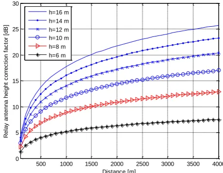
From the previous discussion, it is obvious that one or more parameters need to be taken in account when evaluating . Measurements show, as presented in Fig. 3, that is not only a function of relay antenna height h but it is also a function of distance d. The new relay antenna height correction factor might be expressed as:
(18) where d is the distance in meters between the transmitter and the relay. Fig. 8 presents a family of curves of as a function of distance for different relay antenna heights. If we were to plot path loss curves using (15) and (18) for h= 4, 8, 12 or 16 meter, we will get the curves that correspond to those heights as they are presented in Fig. 3 with negligible error. Equation (18), has two coefficients, 22 and 7.47, that are dependent on the environment.
Table V provides a comparison between the models before and after implementing the antenna height correction factor relative to the measurements.
Fig. 8. Relay antenna height correction factor as a function of distance
TABLE V
MODEL COMPARISON BEFORE AND AFTER IMPLEMENTATION OF THE RELAY ANTENNA HEIGHT CORRECTION FACTOR RELATIVE TO THE MEASUREMENTS
Relay height [m]
Mean (µ) in dB Standard deviation (σ) in dB Before After Before After
4 0 0 6.34 6.34
8 0 0.2 4.98 4.65
12 0 0.5 3.81 3.43
16 0 0.1 2.59 2.23
The comparison is made in terms of the mean (µ) and standard deviation (σ) of the prediction error. It is apparent form this table that implementation of the antenna height correction factor does not affect the agreement with the measurements. Since the path loss model for relay height equal to 4 m was taken as a reference for other models, there is no change in its µ and σ before and after implementation of antenna height correction factor. Interestingly, σ for other rely antenna heights are even better after the implementation of the antenna height correction factor. It seems possible that these results are due to the slightly change in their means µ relative to the ones before the implementation of the antenna height correction factor.
4 6 8 10 12 14 16 18 20
0 5 10 15 20 25
Relay antenna height [m]
R
e
la
y
a
n
te
n
n
a
h
e
ig
h
t
c
o
rr
e
c
ti
o
n
f
a
c
to
r
[d
B
]
102 103
60 70 80 90 100 110 120 130 140 150 160
Distance [m]
P
a
th
L
o
s
s
[
d
B
]
h=4 m - Predicted h=8 m - Predicted h=12 m - Predicted h=16 m - Predicted Free Space
500 1000 1500 2000 2500 3000 3500 4000
0 5 10 15 20 25 30
Distance [m]
R
e
la
y
a
n
te
n
n
a
h
e
ig
h
t
c
o
rr
e
c
ti
o
n
f
a
c
to
r
[d
B
]
[image:5.595.61.288.482.663.2] [image:5.595.311.541.557.617.2]Therefore, the model proposed in (15) along with the associated given in (18) presents a general propagation model. This model might be used to predict the path loss value at any particular distance for any given relay station antenna height between 4 m and 16 m which is a suitable range of relay antenna height and within environment similar to one surveyed in the measurement campaign.
V. SUMMARY AND CONCLUSIONS
This paper presented and analysed the results of a path loss measurement campaign in 1900MHz band. The campaign was set up to examine path loss in the relay environment. It was found that the path loss may be modelled successfully with a slightly modified log-distance propagation model. The path loss equation needs to include a distance dependant antenna height correction. The model equation has three major factors (slope, intercept and antenna height correction), that require four environmentally dependent parameters. The parameters may be determined from empirical studies and through the appropriate linear regression process. The model has standard deviation of the prediction error smaller than 6.5 dB for smaller relay heights (~4m) and smaller than 3dB for higher ones (~16m).
ACKNOWLEDGMENT
Authors would like to acknowledge and thank Mr. Sasie Ahmad for help in the data collection process.
REFERENCES
[1] 3GPP, "TR 36.913 V11.0.0: Requirements for further advancements for Evolved Universal Terrestrial Radio Access (E-UTRA) (LTE-Advanced) (Release11)," 2012-11.
[2] R. Pabst, et al., "Relay-based deployment concepts for wireless and mobile broadband radio," IEEE Communications Magazine, vol. 42, pp. 80-89, 2004.
[3] D. Soldani and S. Dixit, "Wireless relays for broadband access [radio communications series]," IEEE Communications Magazine, vol. 46, pp. 58-66, 2008.
[4] 3GPP, "TR 36.814 V9.0.0: Further advancements for E-UTRA physical layer spects (Release 9)," 2010-03.
[5] I. F. Akyildiz, D. M. Gutierrez-Estavez and E. C. Reyes, “The evolution of 4G cellular systems: LTE-Advanced,” Physical Communications 3, pp. 217-244, 2010.
[6] J. M. P. Kyösti, L. Hentilä, X. Zhao, "WINNER II Channel Models," IST-4-027756 WINNER II, D1.1.2 V1.0, September 2007.
[7] G. Senarath, et al., "Multi-hop Relay System Evaluation Methodology (Channel Model and Performance Metric)," IEEE 802.16j-06/013r3, Feb. 2007.
[8] C. Quang Hien, J.-M. Conrat, and J.-C. Cousin, "On the impact of receive antenna height in a LTE-Advanced relaying scenario," 2010 European Wireless Technology Conference (EuWIT), pp. 129-132, 2010.
[9] C. Quang Hien, J.-M. Conrat, and J.-C. Cousin, "Propagation path loss models for LTE-advanced urban relaying systems," 2011 IEEE
International Symposium on Antennas and Propagation (APSURSI),
pp. 2797-2800, 2011.