warwick.ac.uk/lib-publications
A Thesis Submitted for the Degree of PhD at the University of Warwick
Permanent WRAP URL:
http://wrap.warwick.ac.uk/125717
Copyright and reuse:
This thesis is made available online and is protected by original copyright.
Please scroll down to view the document itself.
Please refer to the repository record for this item for information to help you to cite it.
Our policy information is available from the repository home page.
M A E
G
NS I
T A T MOLEM
U N
IV
ER
SITAS WARWICEN SIS
Ground and Space-based Transit Surveys: Exoplanet
Detection and Evaporating Atmospheres
by
Wai Fun Lam
Thesis
Submitted to the University of Warwick
for the degree of PhD Physics
Doctor of Philosophy
Department of Physics
Contents
List of Tables iv
List of Figures v
Acknowledgments vii
Declarations viii
Abstract x
Abbreviations xi
Chapter 1 Introduction 1
1.1 Exoplanets: The Story So Far... . . 1
1.2 Detection Methods . . . 4
1.2.1 Radial Velocity . . . 5
1.2.2 Transit Detection . . . 8
1.2.3 Microlensing . . . 14
1.2.4 Astrometry . . . 16
1.2.5 Direct Imaging . . . 17
1.3 Hot Jupiter and Super-Earth Planets . . . 20
1.3.1 Hot Jupiters . . . 20
1.3.2 Super-Earths . . . 26
1.4 Stellar Activity in Exoplanetary Science . . . 31
1.4.1 Stellar Activity, Rotation and Age . . . 31
1.4.2 Stellar Activity in Photometry . . . 32
1.4.3 Stellar Activity in Spectroscopy . . . 32
Chapter 2 Methods 36
2.1 Spectroscopy . . . 36
2.1.1 Echelle Spectrograph . . . 36
2.1.2 Data Reduction and Spectra Extration . . . 37
2.1.3 Cross-correlation . . . 37
2.1.4 Stellar Noise and Radial Velocity ‘Jitter’ . . . 40
2.2 Photometry . . . 44
2.2.1 Transit Lightcurve Model . . . 46
2.3 Markov Chain Monte Carlo . . . 51
Chapter 3 From Dense Hot Jupiter to Low-density Neptune: The Discovery of WASP-127b, WASP-136b and WASP-138b 54 3.1 Candidate Identification in the WASP Survey . . . 55
3.2 Follow Up Observations . . . 55
3.2.1 Photometry Follow Up . . . 55
3.2.2 Radial Velocity Follow Up . . . 62
3.2.3 Gaia astrometry . . . 70
3.3 Results . . . 70
3.3.1 Host Star Spectral Analysis . . . 70
3.3.2 Host Star Age Estimates . . . 71
3.3.3 MCMC Analysis . . . 72
3.4 Discussion and Conclusion . . . 76
3.4.1 WASP-127 b . . . 76
3.4.2 WASP-136 b . . . 79
3.4.3 WASP-138 b . . . 82
3.4.4 Conclusion . . . 82
Chapter 4 EPIC 206011496 b: A Transiting Rocky Super-Earth 84 4.1 Candidate Detection - K2 Photometry . . . 85
4.2 Follow up Observations . . . 85
4.2.1 Radial Velocity Follow Up - HARPS . . . 85
4.2.2 Direct Imaging Observations . . . 89
4.2.3 Gaia astrometry . . . 90
4.3 Results . . . 90
4.3.1 Spectral Analysis . . . 90
4.3.2 Stellar Rotation . . . 91
4.3.3 Joint Bayesian Analysis withPASTIS . . . 94
4.4 Discussion and Conclusion . . . 96
Chapter 5 The Evaporating Planet WASP-12 b 101 5.1 Motivation . . . 101
5.1.1 The Curious Case of WASP-12 b . . . 101
5.2 Data Selection and Reduction . . . 103
5.3 Analysis and Results . . . 108
5.3.1 Standardise HIRES Spectra . . . 108
5.3.2 Residual Analysis . . . 108
5.4 Discussion and Conclusion . . . 117
5.4.1 Column Density of the Line Profiles . . . 117
5.4.2 Conclusion . . . 123
Chapter 6 Open Cluster Exoplanet Detection Survey 127 6.1 Advantages and Challenges in the Search for Exoplanets in Open Clusters . 127 6.2 Motivation . . . 128
6.3 Observations . . . 129
6.3.1 Multi-Object Spectrograph FLAMES-GIRAFFE . . . 129
6.3.2 Open Clusters and Target Stars Selection . . . 129
6.4 Analysis . . . 132
6.4.1 Spectral Type Identification . . . 132
6.4.2 The Chromospheric Emission of a star . . . 135
6.5 Discussion . . . 143
6.5.1 Chromospheric Activity and Age of Open Clusters . . . 143
6.5.2 Outlook . . . 145
Chapter 7 Conclusion 148 7.1 Summary . . . 148
7.2 Future work . . . 150
Appendix A Supplementary Tables of Chapter 4 154 A.1 Spectral Analysis of EPIC 206011496 . . . 154
A.2 Radial Velocity Measurements of EPIC 206011496 b . . . 156
A.3 Joint Bayesian Analysis of EPIC 206011496 b . . . 164
List of Tables
3.1 Photometric properties of the three host stars WASP-127, WASP-136 and
WASP-138. . . 56
3.2 Follow up photometric observations of 127, 136 and WASP-138. . . 58
3.3 . . . 70
3.4 Stellar parameters of WASP-127, WASP-136 and WASP-138 . . . 71
3.5 Stellar mass and age estimates of WASP-127, WASP-136 and WASP-138 . 74 3.6 MCMC solutions of WASP-127 . . . 77
3.7 MCMC solutions of WASP-136 and WASP-138 . . . 77
4.1 Properties of EPIC 206011496. EPIC 206011496 has a nearby bound com-panion (see text for detailed description), hence values presented in this table are for the blended photometry. The photometric magnitudes listed were used in deriving the SED as described in Section 4.3.3. . . 87
4.2 System parameters of EPIC 206011496 . . . 95
5.1 System parameters of WASP-12 . . . 102
5.2 List of archival Keck/HIRES observations . . . 104
5.3 Measured column densities of Caiiand Nai . . . 124
6.1 Basic properties of the open cluster samples . . . 131
6.2 Parameters of targets with spectral type later than A5 . . . 133
6.3 Chromospheric activity measurements of stars in open clusters . . . 140
A.1 Chemical abundances of EPIC 206011496 . . . 155
A.2 RV measurements of EPIC 206011496 . . . 156
List of Figures
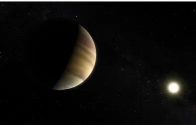
1.1 Artist’s impression of 51 Peg b . . . 2
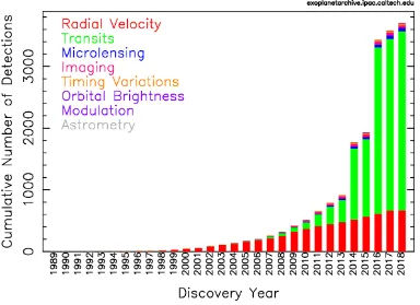
1.2 Cumulative detections of exoplanets . . . 3
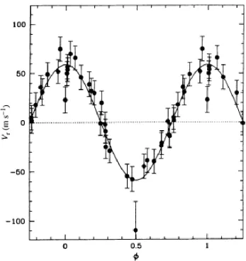
1.3 Radial velocity measurements of 51 Peg . . . 6
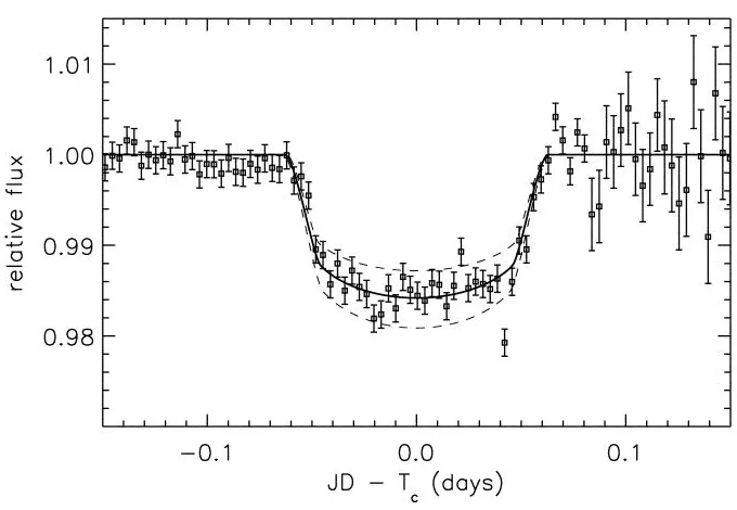
1.4 Phased-folded transit lightcurve of HD209458 b . . . 9
1.5 Analmostedge-on view of a transit event . . . 13
1.6 Microlensing lightcurve of OGLE 2003-BLG-235/MOA 2003-BLG-53 b . 15 1.7 Keck-AO/NIRC2 discovery image of HR8799 e . . . 19
1.8 The masses and orbital periods of currently known exoplanets . . . 22
1.9 The Lyman-αtransit observations of GJ 436. . . 25
1.10 The masses of super-Earths as a function of their equilibrium temperature . 27 1.11 Distribution of planet radii of planets with P<100d . . . 30
1.12 Transit lightcurve of Kepler-30 c . . . 33
2.1 Echelle Spectra Extraction . . . 38
2.2 The line bisector of a CCF profile . . . 41
2.3 Simultaneous RV, S index and photometric observations of HD 166435 . . 43
2.4 Standard lightcurve extraction procedure using aperture photometry and differential photometry. . . 45
2.5 Shape of transit lightcurves under different limb darkening laws . . . 47
2.6 An edge-on view of the geometry of a transit event . . . 49
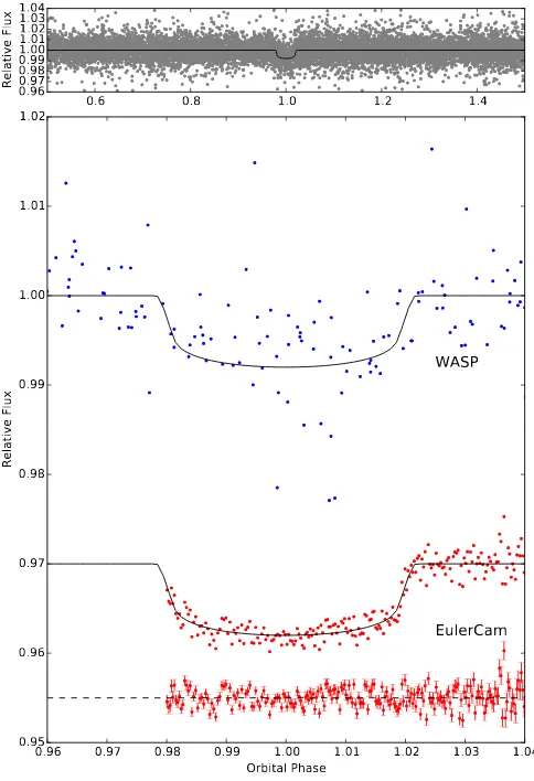
3.1 WASP discovery lightcurve and follow up lightcurves of WASP-127 . . . . 59
3.2 WASP discovery lightcurve and follow up lightcurves of WASP-136 . . . . 60
3.3 WASP discovery lightcurve and follow up lightcurves of WASP-138 . . . . 61
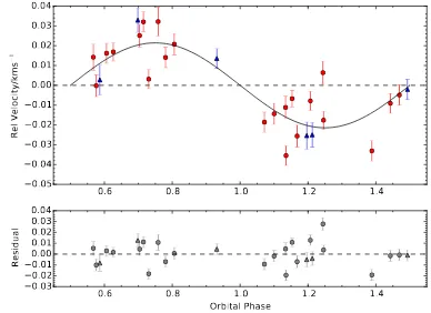
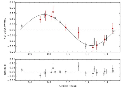
3.4 Phase-folded RV measurements of WASP-127 . . . 63
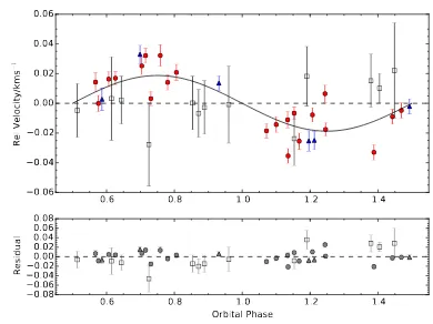
3.5 Phase-folded RV measurements of WASP-127 without the SOPHIE data . . 64
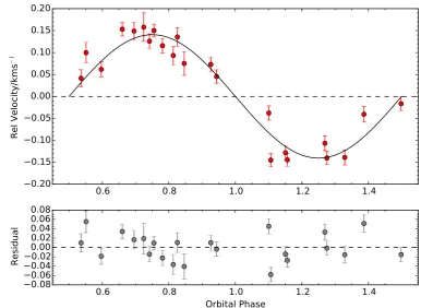
3.6 Phase-folded RV measurements of WASP-136 . . . 65
3.7 Phase-folded RV measurements of WASP-138 . . . 66
3.9 Bisector analysis of WASP-136 . . . 68
3.10 Bisector analysis of WASP-138 . . . 69
3.11 The posterior distribution of the stellar masses and ages . . . 73
3.12 Planet mass as a function of the orbital period . . . 80
4.1 DetrendedK2lightcurve of EPIC 206011496 . . . 86
4.2 Phase-foldedK2lightcurve of EPIC 206011496 . . . 86
4.3 HARPS RV measurements of EPIC 206011496 . . . 88
4.4 K-band Keck AO image of EPIC 206011496 . . . 89
4.5 The auto-correlation function of EPIC 206011496 from the K2 lightcurve . 92 4.6 Lomb-Scargle periodogram . . . 93
4.7 Ternary diagram of the internal composition of EPIC 206011496 b . . . 97
4.8 Planet radius distribution as a function of orbital period . . . 98
4.9 Mass-radius diagram of confirmed exoplanets with masses up to 20 M⊕ . . 100
5.1 WASP-12 model spectrum . . . 109
5.2 Standardised WASP-12 spectrum . . . 109
5.3 Trace residual spectra of WASP-12 centred at CaiiK . . . 112
5.4 Trace residual spectra of WASP-12 centered at CaiiH . . . 113
5.5 Integrated flux in the normalised CaiiH and K residuals . . . 114
5.6 Trace residual spectra of WASP-12 centred at NaiD doublet . . . 115
5.7 Integrated flux in the normalised NaiD residuals . . . 116
5.8 Column densities of Caiiand Nai . . . 118
5.9 Wavelength windows around the Ca iiH & K cores used to calculate the S-index . . . 120
5.10 Reconstructed WASP-12 model spectrum . . . 121
5.11 Residual analysis using reconstructed WASP-12 model . . . 122
6.1 The observed spectrum of TYC6289-1938-1 . . . 137
6.2 TheH1andK1indices for radiative equilibrium (RE) model atmospheres . 138 6.3 Interpolation of Teff andV−Rfrom theB−Vcolour of a star . . . 139
6.4 Chromospheric activity index logR0HK of the open cluster sample . . . 144
Acknowledgments
First and foremost, I would like to thank my supervisor and mentor Don Pollacco for his
guidance and immense patience throughout my PhD. He has provided great support and
ideas during many unscheduled visits, and without him the completion of this PhD would
not be possible.
I am grateful for the assistance and advice offered by the post-docs in the Warwick
Exoplanet group, David Armstrong, David Brown, Francesca Faedi, and James
McCor-mac. In particular, DA and DB for proofreading several chapters in this thesis and provided
constructive feedbacks.
The final stages of a PhD are not easy but I am lucky to have a number of fellow
PhD students who shared this stressful time. James Kirk, Chris Manser, Odette Toloza, and
Louise Wang - thanks for helping me through this period!
Special mention to members of the University of Warwick Volleyball Club for
cre-ating a memorable overall PhD experience. In particular, Zofia Garajova, Marie Grypioti,
Maria Chiara Roffin, Sophia Spadoni, Veronika Vohlmuthova for sharing those coffee
mo-ments.
I thank Andreas Iskra for his valuable discussion on atomic spectroscopy and his
encouragement in the past 3.5 years. You are a star! Last but not least, I would also like to
thank my family for their unconditional support in my decision to continue in academia.
Declarations
I declare that work presented in this thesis is my original research carried out at the
Univer-sity of Warwick during the period from October 2014 to May 2018, under the supervision
of Prof. Don Pollacco. Collaborative work done by others and published work are clearly
indicated in each chapter, and are summarised below.
The work in chapter 3 has been published in the paper by Lam et al. (2017), and
contains some collaborative work. The WASP photometry reduction was performed as part
of the well-established pipeline. Follow up photometric and spectroscopic observations
were obtained by the D.R. Anderson, G. H´ebrard, M. Lendl, L. Mancini, TRAPPIST team,
and A. H. M. Triaud. Spectral analysis was performed by B. Smalley. I was involved in
the candidate detection, stellar age analysis, joint lightcurve and RV analysis for system
characterisation, and lead the publication of the work.
Chapter 4 contains collaborative work in the ESO-K2 consortium. These include
follow up RV and direct imaging observations. The K2 photometry reduction was
per-formed by S. C. C. Barros and D. J. Armstrong. Spectral analysis was perper-formed by
col-laborators at University of Porto, and T. Lopez derived the stellar rotation period using
the stellar activity measurement. Initial MCMC analysis of the planetary system was
per-formed by myself, A. Santerne ran the final and improved MCMC analysis withPASTIS
and the result was adopted in the chapter. I was also involved in the candidate detection,
follow up observations, stellar rotational analysis using the auto-correlation function,
stel-lar ages estimate using gyrochronology and [Y/Mg] ratio, planet composition analysis, and
spearheading the publication of this work.
The WASP-12 HIRES data used in chapter 5 were obtained from the KECK archive. The
candidate selection process in chapter 6 was done by D. J. A. Brown, and the
Abstract
The characteristics and dynamics of exoplanets are broad and diverse. Detailed analysis of the systems can shed light on the history of their formation and evolution. This thesis presents the discovery and analysis of a range of exoplanets. The evaporating planet WASP-12 b was studied to understand the evolution of its atmosphere. Further, the inves-tigation of a new planet detection method through measuring the stellar activity index is presented.
Three gas giant planets were detected by SuperWASP. The inflated Neptune WASP-127 b is one of the least dense planets detected to date. It has a striking atmospheric scale height of 2500 km, which provides an optimal target for atmospheric studies with the James Webb Space Telescope. The hot Jupiter WASP-136 b was found to be in a re-inflation phase as its host star is evolving, and the planet is predicted to have an age of 0.420 Gyr. The detection of WASP-138 b around a slightly metal-poor host weakens the correlation between formation of planets and the metallicity of stars. In addition to ground-based
discoveries, the super-Earth EPIC 206011496 b was detected with the K2 mission. The
mass of EPIC 206011496 b was determined with HARPS RV with a precision of 13%. The bulk density of the planet implies an Earth-like composition which has a predominantly rocky interior. EPIC 206011496 b lies at the lower limit of the photoevaporation gap, which suggests its atmosphere may have been eroded away in the past.
The variability of the evaporating hot Jupiter WASP-12 b was investigated using
archival KECK/HIRES spectra. Enhanced absorption in the cores of both Caii H and K
and NaiD lines were detected throughout the planetary orbit, supporting the presence of a
circumstellar gas disc formed by the evaporated planet material. The mean column density of Caiiwas measured as 6×1014cm−2, which indicates an overall circumstellar gas density of 5.83×10⁻¹⁴g cm−3.
Abbreviations
2MASS . . . Two Micron All–Sky Survey
AO . . . Adaptive optics
APASS. . . AAVSO Photometric All–Sky Survey
BIS . . . Bisector velocity span
BLS . . . Box-least squared algorithm
CCD . . . Charge–coupled device
CCF . . . Cross-correlation function
CHEOPS . . . CHaracterising ExOPlanet Satellite
CoRoT. . . Convection, Rotation and planetary Transits
COS . . . Cosmic Origin Spectrograph
EPIC . . . Ecliptic Plane Input Catalogue
ESO . . . European Southern Observatory
EW . . . Equivalent width
FLAMES . . . Fibre Large Array Multi Element Spectrograph
FoV. . . Field of view
FWHM . . . Full width half maximum
HARPS . . . High Accuracy Radial velocity Planet Searcher
HIRES. . . High Resolution Echelle Spectrometer
HJD . . . Heliocentric Julian Date
HST . . . Hubble Space Telescope
JWST . . . James Webb Space Telescope
MCMC . . . Markov–chain Monte Carlo
NASA. . . National Aeronautics and Space Administration
NUV . . . Near–ultraviolet
RV . . . Radial velocity
SNR . . . Signal–to–noise ratio
STIS . . . Space Telescope Imaging Spectrograph
TESS . . . Transiting Exoplanet Survey Satellite
UTC . . . Universal time coordinated
VLT . . . Very Large Telescope
WASP . . . Wide Angle Search for Planets
Chapter 1
Introduction
1.1
Exoplanets: The Story So Far...
Astronomers have wondered for many years whether there are planets beyond our Solar System. Yet, technical challenge of detecting a low-mass, low-luminosity object in very
close proximity to a star have been the barrier in the race to hunt for exoplanets. The first
breakthrough came about in 1992 when Wolszczan and Frail (1992) confirmed the first
de-tection of exoplanets around the millisecond pulsar PSR1257+12 with radio pulsar timing.
A few years later, 51 Peg b (Mayor and Queloz, 1995) was discovered with the radial
veloc-ity (Doppler) method using high precision fibre-fed spectrograph ELODIE (Baranne et al., 1996). 51 Peg b has a mass of 0.5 MJupand an orbital period of 4.2 days, and is the first exoplanet known to orbit a main sequence star. What was surprising, of course, was the
period and mass of the object - a hot Jupiter. The detection of such an unusual exoplanetary body had sparked great interest in astronomy, and by the end of the decade, a dozen
exo-planets were discovered. Most notably, the first transiting hot Jupiter HD 209458 b (Henry
et al., 2000; Charbonneau et al., 2000) was found, confirming the capability of the transit technique (Borucki and Summers, 1984; Borucki et al., 1985) in exoplanet searches. HD
209458 b went on to become the first planet to have its atmosphere detected and charac-terised with modern spectroscopic techniques (Charbonneau et al., 2002).
With the advancement of technologies and detection methods, much progress has
been made over the past two decades. Multiple detection techniques are well established for
efficient searches of planets: radial velocity measurements (Section 1.2.1), photometry and
transit observations (Section 1.2.2), microlensing (Section 1.2.3), astrometry (Section 1.2.4)
and direct imaging (Section 1.2.5). At the time of writing, 3706 validated exoplanets were discovered (Figure 1.2). The radial velocity and transit detection methods are responsible
Figure 1.1: Artist’s impression of 51 Peg b (left), the first hot Jupiter around a main
se-quence star (right). (Image credit: ESO/M. Kornmesser/Nick Risinger (skysurvey.org))
find periodic fractional changes in the flux of a star, and to determine the size of a planet.
Both space (e.g. Kepler; Borucki et al. 2010 and K2 missions; Howell et al. 2014) and
ground-based (e.g. HATNet; Bakos et al. 2002, SuperWASP; Pollacco et al. 2006, KELT;
Pepper et al. 2007, HATSouth; Bakos et al. 2013, NGTS; Wheatley et al. 2013) transit
surveys have provided a huge sample of exoplanets for statistical studies and detailed char-acterisations. On the other hand, the radial velocity technique relies on the orbital reflex
motion of the star-planet pair to constrain the planetary mass. The precision of this method depends heavily on the stability and resolution of spectrographs. From ELODIE (Baranne
et al., 1996), to CORALIE (Queloz et al., 2000; Pepe et al., 2002a), and HARPS (Queloz
et al., 2001b; Pepe et al., 2002b), the advances in instruments throughout the years have
improved precisions of measurements down to below 1 m s−1.
The radial velocity and transit observations are often made to compliment each other
in planet detections. Detailed analyses of these observations have revealed a diverse range of exoplanets, many of which have characteristics that are unobserved in our Solar
Sys-tem. New theoretical challenges have emerged, and formation and evolution mechanisms
of different types of planet populations are yet to be understood.
Hot Jupiters are gas giants which orbit their host stars with periods of≤ 10 days,
range in radii from 0.775 RJ (WASP-59b; H´ebrard et al. 2013) to 1.932 RJ (WASP-17b; Anderson et al. 2010; Southworth et al. 2012). Many of these hot Jupiters were found to
have radii larger than predicted from standard coreless models (e.g. Fortney et al. 2007). Several theories were proposed to explain the observed inflated radii. These include stellar
irradiation (Guillot et al., 1996), tidal heating (Bodenheimer et al., 2001, 2003), enhanced
atmospheric opacity (Burrows et al., 2007), and Ohmic heating (Batygin et al., 2011). On the opposite end of the spectrum, super-Earths are planets with sizes between
the Earth and Neptune. From what we know from discoveries to date, they appear to be the
most abundant type of exoplanet in our galaxy. Statistical studies have shown that 13% of
main sequence GK stars host a super-Earth with orbital period< 50 days (Howard et al.,
2012). Theoretical predictions showed differing evolution mechanisms can lead to a
tran-sition region among super-Earths, which separates the two distinct families with differing
radii and compositions (e.g. Lopez et al. 2012; Lopez and Fortney 2013; Owen and Wu
2013). Planets with radii RP ≤ 1.6 R⊕(e.g. Kepler-10 b; Batalha et al. 2011, LHS1140 b;
Dittmann et al. 2017) have higher bulk densities, and would possess a predominantly rocky interior. Whereas planets with lower densities (e.g. GJ 1214 b; Charbonneau et al. 2009,
Kepler-11 system; Lissauer et al. 2011a) are more likely to bear solid cores and substantial gaseous envelopes.
Meanwhile, there is also a number of short-period sub-Saturn and super-Neptune
mass planets such as WASP-39b (Mp = 0.28 MJ; Faedi et al. 2011), HAT-P-11b (Mp =
0.081 MJ; Bakos et al. 2010), and HAT-P-26b (Mp = 0.059 MJ; Hartman et al. 2011).
In the short-period planet population, there is a significant lack of detected planets with
sizes between Jupiter and the Earth, giving rise to the so-called ‘Neptune desert’ (Mazeh et al., 2016). The presence of these intermediate planets are test beds for theories as to
differentiates the formation and evolution histories of planet populations.
With the expanding number of exoplanets, it appears more questions emerged than are answered. However, future missions such as CHEOPS (Broeg et al., 2013), TESS
(Ricker et al., 2014), PLATO (Rauer et al., 2014), along with future generations of
spectro-graphs and near-infrared instruments, e.g. ESPRESSO (Pepe et al., 2014) and CARMENES Quirrenbach et al. 2012, we can obtain exceptional precision in radial velocity and transit
measurements to aid our understanding in the present structures and dynamics of planets
beyond our Solar system.
1.2
Detection Methods
notable discoveries and their detection parameter spaces are discussed.
1.2.1 Radial Velocity
The radial velocity (RV) detection technique first revealed the existence of planets around
sun-like stars beyond our Solar System (Mayor and Queloz, 1995). It relies on the
mea-surement of a star’s reflex motion. In the presence of a planetary companion, the star orbits about the system’s barycentre due to the planet’s gravity. This results in a RV variation of
the star, i.e. the change in velocity of the star towards and away from the observer (Mayor
et al., 2014). Radial velocities can be measured using the Doppler shift of stellar absorption lines. Lines are redshifted (resulting in positive RV signals) if the distance between the star
and the observer is increases. Meanwhile, lines are blueshifted (giving negative RV signals)
when the distance between the star and the observer is reduced.
For a planet of mass Mp in an orbit with semi-major axis,a, eccentricity, e, and a
period,P, theradial velocity signalof the star is (Wright and Howard, 2009; Perryman,
2014):
νr(t)=K[cos (ω+ν(t))+ecosω]+γ+d(t−t0) (1.1)
whereγ is the time-independent velocity offset, anddis the linear trend parameter which
accounts for the instrumental drift and/or contribution from a massive companion. The
argument of pericentreωis the angular coordinate of the orbiting body’s pericentre relative
to the orbital plane and direction of motion. The true anomaly ν(t) measures the angle
between the pericentre and the current position of the body. Kis theradial velocity
semi-amplitude, which is expressed as:
K = 2πG
P
13 Mpsini
(Ms+Mp)2/3(1−e2)1/2
(1.2)
The orbital inclination is denoted byi,Gis the Gravitational constant,MsandMpare the
masses of the star and planet, respectively. The semi-amplitudeKis dominated by the term
Mpsini, meaning the radial velocity method is more sensitive to massive planets.
The star’s motion about the barycentre can be measured using theDoppler shiftof
stellar absorption lines. The shift in wavelength is:
∆λ= λobs−λrest
λrest
(1.3)
In the Solar System, the RV semi-amplitude of the Sun due to Jupiter’s gravity is
12 m s−1(Mayor et al., 2014). A precise measurement of the RV amplitude of the star can
Figure 1.3: Radial velocity measurements of 51 Peg (phased atP = 4.5 d) show a
semi-amplitude of 0.059±0.003 ms−1(from Mayor and Queloz (1995) reprinted with permission
result in a larger RV variation. In a system where a 10 Jupiter-mass (MJ) planet orbits a
solar-mass star, the corresponding RV semi-amplitude is 1.0 km s−1(Bouchy et al., 2009b).
A brown dwarf can have a mass as low as 30MJ. Hence, a RV amplitude of larger than a
few km s−1indicates the likelihood of a stellar companion instead of a planet.
Giant planets shift the velocities of the host star by tens of m s−1, therefore high
precision spectrographs are necessary to reveal the accurate masses of exoplanets. The use of CORAVEL (Baranne et al., 1979) showed that Doppler motions of stars can be derived
using the cross-correlation method. This knowledge was applied for the development of
ELODIE (Baranne et al., 1996), a fibre-fed cross-dispersion spectrograph located on the 1.93 m telescope at the Observatoire de Haute-Provence (OHP). The instrument was able to
achieve a radial velocity precision of∼15 m s−1, and 51 Peg b was soon discovered (Mayor
and Queloz, 1995).
The SOPHIE spectrograph (Bouchy et al., 2009a) has replaced ELODIE since 2006.
The spectrograph operates with a spectral resolution of 75,000 and a coverage between 387
- 694 nm. It can derive RV measurements with a precision between 1 and 2 m s−1.
The CORALIE spectrograph (Queloz et al., 2000; Pepe et al., 2002a) was installed
at the 1.2 m Euler-Swiss Telescope at the ESO La Silla Observatory, Chile, following the
success of ELODIE. With a resolving power of 50,000, the instrument can obtain RV
mea-surements with a precision of∼few m s−1. SOPHIE and CORALIE spectrographs were
instrumental in the follow-up effort for exoplanet detection in the past decade. Coupled
with ground-based transiting surveys such as SuperWASP (to be discussed in detail in
Sec-tion 1.2.2), and NGTS, accurate mass estimates of Jupiter and sub-Saturn mass planets can
be achieved for detailed system characterisation.
The development of these spectrographs has demonstrated the need for a stable
spectrograph to obtain 1 m s−1precision RV measurements to constrain masses of Neptune
and Earth mass planets. The HARPS (High Accuracy Radial velocity Planet Searcher)
spectrograph mounted on the 3.6 m Telescope at ESO La Silla Observatory (Mayor et al.,
2003) was designed for this specific purpose. The first HARPS discovery was the hot Jupiter
HD 330075 b with minimum mass of 0.62 MJ(Pepe et al., 2004), where measurements were
reported to have a root-mean-squared (rms) velocity of only 2 m s−1. Further success came
when HARPS reported the discovery of the super-EarthµAra b (Santos et al., 2004). The
star was reported to have a semi-amplitude of just 4.1 m s−1, and HARPS was capable of
measuring radial velocities with precision better than 1 m s−1. Early HARPS RV survey
have also shown that low-mass planets are common in multiplanet systems. HARPS-N
(Cosentino et al., 2012) on the 3.5 m Telescopio Nazionale Galileo (TNG) also provided
accurate mass measurements for many Kepler/K2 planetary candidates. The development
Exoplanets and Stable Spectroscopic Observations: Pepe et al. 2014), and near infra-red
spectrographs/spectropolarimeters (e.g. CARMENES: Quirrenbach et al. 2012, SPIRou:
Delfosse et al. 2013), will be able to search for low-mass rocky planets in the habitable zones of quiet G - M dwarfs.
1.2.2 Transit Detection
The transit detection method remains the only direct route to determine planetary radius.
The STARE telescope produced the first full transit observation of exoplanet (Charbonneau
et al., 2000). From the two transits obtained, Charbonneau et al. were able to infer the planetary radius (Rp =1.27±0.02 RJ), as well as the orbital period (P=3.52 d) and orbital
separation (a = 0.0467 AU) of the system. Since then, the field of transit photometry
has expanded significantly. The cost and accessibility of the transit detection method is relatively lower than for RV surveys. Many wide-field transit surveys have been established,
yielding many interesting exoplanets with sizes ranging from Jupiter radii down to
super-Earth radii.
Ground-based Surveys
Ground-based surveys provided a large number of candidates around stars that are suffi
-ciently bright to enable follow up RV measurements, where strong observational constraints are obtained for theoretical studies.
Most transit detection surveys adopt the following sequence to identify candidate
planets: Detection surveys monitor tens of thousands of bright stars with V < 13 mag
over a long period of time. The photometric data obtained are then reduced with aperture
photometry using custom built pipelines. To correct for trends and systematic errors, the lightcurves are fitted with trend-removing algorithms to decorrelate systematic errors (e.g.
SysRem: Tamuz et al. 2005, TFA: Kov´acs et al. 2005, EPD: Bakos et al. 2010). A
box-firring least squares algorithm (BLS: Kov´acs et al. 2002) is applied to estimate the transit epoch, period, depth, and duration, such that periodic box-like signals can be identified.
After a series of rigorous elimination of false positives (e.g. eclipsing binaries and giants),
the best planetary candidates are subjected to follow up photometry and radial velocity observations for further detailed analyses.
SuperWASP(Wide Angle Search for Planets; Pollacco et al. 2006) is one of the
most successful ground-based transit surveys. The WASP-North facility is located at the Observatorio del Roque de los Muchachos in La Palma, Canary Islands, and the
WASP-South facility is located at the Sutherland Station of the WASP-South African Astronomical
Figure 1.4: Phased-folded transit lightcurve of HD209458 b from Charbonneau et al.
coupled with e2v CCDs of 2048×2048 pixels each. The cameras in each facility provide a
total field of view (FoV) of 8×64 square degrees and a pixel scale of 13.7”. The telescopes
can survey millions of objects and achieve a photometric precision better than 4 mmag for
stars brighter than V∼ 9.4 mag, and an accuracy of 1% for starts brighter than V∼ 11.5
mag.
To date, over 150 exoplanet discoveries have been made with WASP, and a diverse population of planetary systems has been revealed. The Saturn-mass planet WASP-17 b
(Anderson et al., 2010; Southworth et al., 2012) was found to be an inflated planet due to
tidal heating from the tidal circularisation of its eccentric orbit. The Rossiter-McLaughlin
effect was observed in the WASP-17 system, suggesting the planet is misaligned with a
spin orbit angle ofψ > 91.7◦, hence a retrograde orbit (Triaud et al., 2010). Another low-density Saturn WASP-39 b was reported by Faedi et al. (2011) and a clear atmosphere was detected on this inflated planet (Sing et al., 2016; Barstow et al., 2017). WASP-12b is one
of the hottest Jupiter known with an equilibrium temperature of 2516 K (Hebb et al., 2009).
An enhanced transit was detected in the Near-UV (Fossati et al., 2010b). Further spectral analyses have shown complete absorption in the Mg II h & k and Ca II H & K line cores
(Haswell et al., 2012; Fossati et al., 2013), suggestive of an extended exosphere around the planet WASP-12 b. The analysis of the time variability of the atmosphere of WASP-12 b
will be discussed in more detail in Chapter 5.
HAT/HATNet(Hungarian Automated Telescope project; Bakos et al. 2004) com-prises of the HATNorth and the HATSouth network. There are six automated telescopes at
the HATNorth network, four of which are based in the Fred Lawrence Whipple Observatory
(FLWO), a further two at the Submillimeter Array of SAO in the Mauna Kea Observatory. The HATSouth network is formed of six telescopes in the southern hemisphere. They are
located at the Las Campanas Observatory (LCO), Chile, the High Energy Spectroscopic
Survey (HESS) in Namibia, and the Siding Spring Observatory (SSO) in Australia.
Many interesting planets have been detected by HATNet. HAT-P-11b (Bakos et al.,
2010) was the first transiting Neptune discovered from ground-based surveys. Transmission
spectrum of HAT-P-11b revealed a cloud-free atmosphere on the planet and the presence of water vapour in its atmosphere. The irradiated massive hot Jupiter HAT-P-7b (Hartman
et al., 2011) is a highly tilted planet with a retrograde orbit (Winn et al., 2009). The
opti-cal phase curve measurement of the system also found the planet’s day-side temperature as
2650±100 K (Borucki et al., 2009).
Ground-based surveys continue to make groundbreaking discoveries. SuperWASP
and HATNet, along withKELT(Pepper et al., 2007),QES(Alsubai et al., 2013),NGTS
Evryscope(Law et al., 2015) andFly’s Eye Camera(P´al et al., 2016) will be able to push
detection boundaries and search for smaller planets around brighter stars. These targets are
crucial for characterisation with the James Webb Space Telescope in the near future.
Space-based Surveys
While ground-based projects have provided bright targets for follow up characterisations,
the accuracies of transit lightcurves are limited by factors such as atmospheric extinction and scintillation. The planet detection parameter space is restricted to those with sizes of
Jupiter or Neptune at best. Fortunately, the launch of space-based missions in the past
decade meant that high precision photometry can be obtained, enabling the detection of sub-Neptune and Earth-sized planets.
The CoRoT satellite (Barge et al., 2008; Auvergne et al., 2009) commissioned
be-tween 2007 and 2012 was the first dedicated mission to search for transiting exoplanets in space. The telescope observed over 60,000 stars with a photometric precision of 7×10⁻⁴at
V= 15.5 mag for a one hour integration. With this unprecedented precision, the first
tran-siting super-Earth was discovered by L´eger et al. (2009). The transit lightcurve of CoRoT-7 b revealed a planet with a size 1.68 times larger than the Earth and an orbital period of
0.85 d. The mass of the planet, however, has been disputed over the years. Queloz et al.
(2009) determined the planet mass as 4.8±0.8 M⊕using follow up RV data from HARPS.
Fourier analysis of the HARPS data by Hatzes et al. (2010) argued that the RV signal of
CoRoT-7 b suggested the planet has a mass of 6.9±1.4 M⊕. Further reassessment of the
RV data by Pont et al. (2011), Boisse et al. (2011b), Hatzes et al. (2011), and Ferraz-Mello
et al. (2011) showed a varied mass range of 1 - 8 M⊕. One valuable lesson learnt from this
system was the importance of understanding the role of stellar activity and radial velocity jitter in the planetary system analysis. Accurate mass derivation is particularly important in
the determination of the interior structure of an Earth-like planet.
Following the launch of the CoRoT satellite, theKepler mission was launched in
2009 (Borucki et al., 2010; Koch et al., 2010) with a primary goal to determine occurrence
rates, sizes and orbital separations of habitable Earth-sized planets. The telescope
com-prises of a 0.95 m aperture Schmidt telescope with an array of 42 1k×2k CCDs, giving a
total FoV of 113 square degrees. The instrument can acquire transit lightcurves with a
pre-cision of 10 ppm per 6hours for V=10 stars. The Kepler mission has thus far detected over
4000 transiting planet candidates, enabling statistical study on planet populations. Not only did the Kepler studies revealed that most stars have planets, it also found that small planets
with radius RP < 4.0 R⊕are by far the most common type of planets in the galaxy (e.g.
The mission came to an end in 2013 when the second reaction wheel on the satellite
failed, and the extended surveyK2mission (Howell et al., 2014) was adopted to continue
with transiting exoplanet searches. K2has the ability to obtain a photometric precision of
80 ppm at V = 12 mag in a 6-hour integration. So far, the mission has completed sixteen
observational campaigns, producing over 20,000 lightcurves per campaign. At the time of
writing,K2has identified hundreds of candidates (e.g. Vanderburg et al. 2016; Barros et al.
2016; Pope et al. 2016) and over 200 validated planets (e.g. Montet et al. 2015; Barros et al.
2015; Crossfield et al. 2016).
The discoveries made withKepler/K2showed a variety of bulk densities in
Earth-mass planets. For example, both Kepler-10 b (RP=1.42±0.03 R⊕,ρP =8.8±2.5 g cm−3;
Batalha et al. 2011) and K2-38 b (RP=1.55±0.02 R⊕,ρP=17.5±7.35 g cm−3; Sinukoff
et al. 2016) are planets with densities higher than the Earth and internal compositions which resemble a rocky world. At the same time, there are planets which were found to possess
solid cores and massive gaseous envelopes (e.g. Kepler-11 system: RP = 1.97-4.52R⊕,
ρP = 0.5-3.1 g cm−3; Lissauer et al. 2011a, K2-18 b: RP=2.28±0.03 R⊕,ρP = 3.3±1.2
g cm−3; Benneke et al. 2017; Cloutier et al. 2017).
Very soon, the next generation of space missions will be commissioned. The Tran-siting Exoplanet Survey Satellite (TESS: Ricker et al. (2014)) was launched in April 2018.
TESS contains four wide-field optical 4k×4k CCDs, each providing a 24×24 square
de-grees FoV. The mission will monitor 200,000 bright stars (I∼4 - 15) to obtain lightcurves
with a precision of∼ 200 ppm per 1 hour for V= 10 stars. The Characterising Exoplanet
Satellite (CHEOPS; Broeg et al. 2013) is set to launch in December 2018. The mission will
provide precision photometry (precision of 20 ppm per 6 hours for bright stars of V = 9
mag) for transit follow up on bright targets. It will be able to provide radii estimates of small
planets with an accuracy of better than 10%. The PLAnetary Transits and Oscillations of
stars mission (PLATO: Rauer et al. (2014)) is a transit survey anticipated to launch in 2026. The goal of the mission is to detect and characterise habitable zone planets. To fully
char-acterise a system, the planet’s mass and radius, and the stellar age must be derived with a
high accuracy. PLATO will target bright stars with V ≤ 11 mag to obtain high precision
lightcurves, where planetary radii with an accuracy of∼2% can be achieved. Furthermore,
the lightcurves will be analysed with asteroseismology to constrain stellar ages with a
pre-cision of 10%. Bright targets also means that ground-based spectroscopic instruments can make RV measurements with accuracies of 4 - 10% to achieve the end goal of finding an
Figure 1.5: Analmostedge-on view of a transit event (reproduced from Winn (2009) with
permission fromInternational Astronomical Union). When a planetary object orbits around
a star, the planet will block part of the stellar flux when it passes between the observer and the star. The flux will drop again at the secondary eclipse when the planet is occulted by the star. Four parameters can be observed during a transit event: the mid-transit timetc, the
transit depthδ, the total transit durationT, and the ingress or egress durationτ.
Interpreting the Transit Lightcurve
A transit lightcurve can provide a wealth of information about an exoplanet system. Here,
the physical parameters that can be inferred from a lightcurve are summarised.
The transit lightcurve in Figure 1.5 shows four of the parameters which can be
measured directly from observations, namely, the mid-transit timetc, the depthδ, the total
durationT , and the ingress or egress durationτ(Winn, 2009).
If a planet with radiusRporbits a star with radiusRs, thestar-planet size ratiocan
be measured approximately by the depth of the transit:
δ= ∆F
F =
R2P
R2S (1.4)
where F is the flux of the star and∆F is the fraction of flux blocked by the planet. The
Rs
a =
π√Tτ
δ1/4P
1+esinω p
1−e2
(1.5)
whereωis the argument of pericentre, which can be obtained from RV measurements. The
massMsand radiusRs of a star can be estimated from spectral analysis. Using Kepler’s
third law, thesemi-major axis,a, can be inferred:
a3
P2 =
G(Ms+Mp)
4π2 (1.6)
For a planet moving in a circular orbit, the orbital velocity is v = 2πa/P. The
impact parameterbis defined as the vertical distance between the centre of the stellar disc
and the centre of the planet:
b≡ a
Rs
cosi=1− √δT
τ (1.7)
whereiis the orbital inclination. Furthermore, Kepler’s third law can be applied to
deter-mine thestellar mean densityρs:
ρs≈
3P
π2G √
δ
Tτ
3/2 1−e
2
(1+esinω)2 3/2
(1.8)
and theplanet surface gravitygpis:
gp≈
2πK P
p 1−e2
δ(Rs/a)2sini
(1.9)
Whether a transit can be detected depends on the geometry of the system. The probabilityPtranof detecting a transiting planet on a circular orbit is:
Ptran =
Rs+Rp
a ≈
Rs
a (1.10)
Thus the transit method is highly biased towards systems with close-in orbits, which partly
explains the abundance of short period planets discovered via transit photometry.
Further details on transit lightcurve model fitting and characterisation of planetary
systems will be discussed in Chapter 2, 3, and 4.
1.2.3 Microlensing
Gravitational lensing is the effect when a massive object (the lens) bends the path of light
from a background source (Einstein, 1936). Under special circumstances, multiple distorted
images are formed milliarcseconds apart. Although lensing events are difficult to resolve,
observable magnification event. Microlensing survey began to take form when Paczynski
(1986) presented the possibility of detecting dark matter in the halo of our Galaxy. Later,
Mao and Paczynski (1991) showed that the microlensing technique may also be applied to binaries and planetary companion. If a lensing star has a planetary companion which also
aligns with the primary lensing event along our line-of-sight, it would perturb the image and
produce a sharp spike in the microlensing lightcurve. Mao and Paczynski (1991) predicted the probability of microlensing event by planetary systems to be 0.03, assuming the star-to-planet mass ratio as 103.
Figure 1.6: Microlensing lightcurve of OGLE 2003-BLG-235/MOA 2003-BLG-53 b. The
blue open circles and red filled circles shows the OGLE and MOA measurements respec-tively. The best-fit binary microlensing model is plotted as the black solid line, and the single-lens model is plotted in cyan. (Figure reproduced from Bond et al. (2004) with
per-mission byThe American Astronomical Society.)
first microlensing planet detection only came about in 2004 (Bond et al., 2004). Information
such as the mass ratio of the star planet system, mass of the primary lens (i.e. the star), and
the orbital separation of the pair can be derived. Figure 1.6 shows the discovery data from OGLE (Optical Gravitational Lensing Experiment; Udalski (2003)) and MOA
(Microlens-ing Observations in Astrophysics; Bond et al. (2001)), a mass ratio of q = 0.0039 was
found, and OGLE 2003-BLG-235/MoA 2003-BLG-53 b was determined to have a mass of
1.5 MJand an orbital separation of∼3 AU.
Multi-planet systems are also detectable using the microlensing method. Gaudi
et al. (2008) discovered the planetary system OGLE- 2006-BLG-109L which consists of
two Jupiter and Saturn-like planets. The planets were determined to have masses of ∼
0.71 MJand∼0.27 MJ, respectively. Furthermore, these planets have orbital separations of
∼2.3 AU and∼4.6 AU, which makes them comparable to planets within the Solar System.
Over 50 exoplanets have been detected by the microlensing method today. Although
the detection probability of this technique is relatively low as it is more sensitive to planets
near the Einstein ring radius of the lens, the microlensing method have weaker selection biases compared to other detection methods. Microlensing discoveries have proved that the
method is sensitive to long period, low-mass planets orbiting beyond the snow line. It can therefore probe regions of the mass-radius parameter space which are otherwise challenging
for transit and radial velocity methods. Many microlensing discoveries resemble planets in
our solar system. They can provide important constraints on the occurrence of solar system analogues.
1.2.4 Astrometry
Bodies in a planetary system orbit around a common centre of mass (i.e. the barycentre of
the system). Similar to the radial velocity method, astrometry quantifies the gravitational
perturbation of the host star due to its companion by measuring the relative position of the
star (Perryman, 2014). The elliptical motion of the star has a semi-major axisasof
as=
Mp
Ms
!
a (1.11)
The observableastrometric signaturein the astrometry method is therefore the
an-gular displacementαof the stellar orbit
α= Mp
M∗ ! a 1AU d 1pc !−1
arcsec (1.12)
wheredis the distance of the object from the observer. As seen in Equation 1.12, the
technique is more sensitive to long period systems. However, this method is severely
lim-ited by the accuracy of the positional measurement of a star. At a distance of 100 pc, a
Jupiter analogue would have a signatureα = 50 µas, and an Earth analogue would have
α=0.03µas. The astrometry method thus requires a precision of sub-mas for planet
detec-tions.
Space astrometry is able to measure trigonometric parallaxes of objects. The Hip-parcos mission provided measurements of positions, proper motions, and parallaxes of
120,000 stars with a 1 mas accuracy between 1989 and 1993 (Perryman et al., 1997). The
Fine Guidance Sensor (Benedict et al., 1998) on the Hubble Space Telescope can measure
parallaxes at∼ 1-2 mas precision. Gaia (Perryman et al., 2001) is the successor of the
Hipparcos mission. It surveys∼ 1 billion stars to determine the positions of the Galactic
stellar populations. With an accuracy of∼ 10 µas, it is expected to yield approximately
21,000 exoplanets out to a distance of∼ 500 pc, including low-mass planets with masses
of∼10 M⊕(Perryman et al., 2014), for a 5 year mission.
Radial velocity can only provide the Mpsiniestimate and give a minimum mass
limit of the planetary companion since the orbital inclinationiis undefined. Astrometric
measurements, however, can determine the precise value ofi. The combined analysis of the
two methods will place constraints on the companion mass, thus reveal the true mass of the
planet. Using the true planet mass and a well constraint planet radius, one can determine
the planet bulk density precisely, hence infer the interior composition of the planet. In particular, the ice-mass fraction of a planetary core allows us to determine if a planet was
formed beyond the snowline or assembled locally (Jin and Mordasini, 2018), the formation
and evolution history of a planetary systems can then be inferred (e.g. GJ 317; Anglada-Escud´e et al. (2012)).
1.2.5 Direct Imaging
Most of the exoplanets known to date were discovered by making measurements of systems
indirectly. Only a handful of objects were confirmed with direct imaging. The main
ob-stacles encountered in this method are the extreme star-to-planet contrast ratio, the angular separation of the planet, and the quasi-static speckle noise.
A planet with radiusRp and orbital separationacan reflect a fraction (Rp/2a)2 of
the star’s luminosity at wavelengthλ. The observed planet-to-star flux ratio is therefore
fp(α, λ)
fs(λ) =
p(λ) Rp a
!2
g(α) (1.13)
from the Earth, the contrast ratio fp/fs would be∼ 10−9, and the system would have an
angular separation of 0.5 arcsec. To image the planetary companion, the contrast ratio and
the angular resolution must be significantly improved. This can be done by making ob-servations in the infrared to limit stellar emission while increasing thermal emission from
the planet. Again for a Jupiter analogue around a Sun-like star, this contrast ratio can be
improved to∼ 10−4. Another way to increase the contrast ratio is to apply a coronagraph
to the telescope which masks the flux of the on-axis star, the flux and structure from the
off-axis companion would remain (Lyot, 1939). Meanwhile, the angular resolution of the
observations can be enhanced through adaptive optics (AO) on ground-based instruments or by making observations from space.
The contrast ratio detection limit in direct imaging is ultimately determined by
speckle noise. Speckle noise can arise due to instrumental flaws and atmospheric turbu-lence, which can produce interference patterns and hide planetary signals in images (Racine
et al., 1999). A number of post-processing techniques have been developed to suppress
speckle noise. The most widely adapted technique is Angular Difference Imaging (ADI:
Marois et al. 2006), where the FoV is allowed to rotate around the star while the telescope
rotator is fixed. The speckle pattern correlated to the instrument is then subtracted from images to remove the noise.
Many of the present day direct imaging surveys are ground-based. To optimise
the sensitivity, a Lyot coronagraph is combined with an AO system for wavefront
correc-tion (Malbet, 1996; Sivaramakrishnan et al., 2001), e.g. VLT/NACO (Rousset et al., 2000;
Chauvin et al., 2015), Keck-AO/NIRC21, Gemini South/NICI (Chun et al., 2008; Liu et al.,
2010), and Subaru-CIAO (Tamura et al., 2001; Murakawa et al., 2004). The first directly
imaged exoplanet was discovered using this combined technique. The 5MJ planet 2M1207
b was detected by VLT/NACO (Chauvin et al., 2004). It was found to orbit a brown dwarf
with a separation of∼55 AU. High contrast AO observations with Keck and Gemini have
confirmed a multiplanetary system around the A5V star HR8799 (Marois et al., 2008). The
planets HR8799 b, HR8799 c, and HR8799 d were determined to have masses of 7 MJ,
10MJ, and 10MJ, respectively, each with orbital separations of 68 AU, 38 AU, and 24 AU,
from the host star. A forth planet HR8799 e orbiting interior to the other at∼14.5 AU was
reported by Marois et al. (2010) (see Figure 1.7). Another remarkable discovery of a gas
giant planet was imaged in the disk ofβPictoris (Lagrange et al., 2009, 2010).βPictoris b
is at a separation of∼8 AU from the star, and was found to be responsible for clearing the
gap inside the disc.
With the development of extreme AO systems such as VLT/SPHERE
(Spectro-Polarimetric High-contrast Exoplanet Research: Beuzit et al. (2008)) and the Gemini Planet
Figure 1.7: Keck-AO/NIRC2 discovery image of HR8799 e (Marois et al., 2010),
Imager (GPI: Macintosh et al. (2014)), it is possible to extend planet searches down to an
an-gular scale of∼0.1 arcsec. These instruments are coupled with integral field spectrograph,
such that low resolution (R∼ 30 spectroscopy is made available to study exoplanet
atmo-spheres. The first low-resolution near-infrared spectra ofβ Pictoris b obtained from GPI
have shown water absorption features in the planet atmosphere (Bonnefoy et al., 2014), a
prominent characteristic for an early L dwarf.
The launch of the James Webb Space Telescope (JWST; Gardner et al. 2006) is
im-minent. The coronagraphs (MIRI; Boccaletti et al. 2015, TFI; Doyon et al. 2010) on board
the telescope will be able to reach a contrast ratio of 104-105at 0.5-1.0 arcsec separations. The detection of super-Earths around M dwarfs would be possible (Deming et al., 2009).
WFIRST-AFTA (Wide-Field InfraRed Survey Telescope-Astrophysics Focused Telescope
Assets) will contain a coronograph instrument targeted for the imaging and spectroscopy of exoplanets in the solar neighbourhood (Noecker et al., 2016).
1.3
Hot Jupiter and Super-Earth Planets
New classes of planets have been discovered since the first detection of exoplanets. The
detailed analyses of exoplanets have shown systems with properties that are different from
our own Solar system. In this section, properties and characteristics of hot Jupiters and super-Earths are presented. Some interesting questions and key findings are discussed.
1.3.1 Hot Jupiters
Hot Jupiters are Jupiters which orbit close to their host stars with orbital separations of
a < 0.1 AU, periods P≤ 10 days (Udry and Santos, 2007). This type of planet receives
strong stellar irradiation, leading to a high equilibrium temperature. Hot Jupiters are the
easiest exoplanet to find via transits and RV because they are more massive, hence they are
more sensitive to the RV detection method. Indeed, the first exoplanet discovered around a solar-type star is the hot Jupiter 51 Peg b. This astonishing find challenged formation
theories at the time since gas giants were thought to be forms at wider orbits of several
AUs.
How Were Hot Jupiters Formed?
Multiple formation mechanisms were proposed to explain the short orbital periods of hot
Jupiters. Hot Jupiters could have migrated viagas disc migrationor throughhigh-eccentricity
migration. In gas disc migration, planets exchange angular momentum with the gas disc,
Lin 2008). Another type of migration is the high-eccentricity migration. The eccentricity
of a hot Jupiter on a wide orbit is first excited by some physical processes. This could
be planet-planet scattering (Rasio and Ford, 1996; Weidenschilling and Marzari, 1996):
In a system with multiple protoplanets, one of the planets could become sufficiently large
and perturb its smaller rival counterparts. These smaller planets are eventually expelled,
while the largest planet would gain eccentricity in the process; orSecular perturbation:
The Kozai-Lidov mechanism (Kozai, 1962; Lidov, 1962) can drive the angular momentum
exchange between the hot Jupiter and an eccentric outer planet body or a star, resulting in
the excitation of the hot Jupiter’s eccentricity. When the orbit of a hot Jupiter becomes eccentric, the planet would lose orbital energy through tidal dissipation (i.e. tides raised on
the planet by the star), the planet orbit is consequently circularised. Although the
forma-tion mechanisms of hot Jupiters is still unclear, a more complete study of the hot Jupiter population may shed some light on their origins.
Hot Jupiter Occurrence and Some Distinct Characteristics
The radial velocity survey by Mayor et al. (2011) reported an occurrence of 0.89% for hot
Jupiters around main-sequence stars. The California Planet Survey (Wright et al., 2012)
found a rate of 1.2%, while Batalha et al. (2013) estimated a rate of 0.5% for hot Jupiters in the Kepler sample. These surveys showed that hot Jupiters are intrinsically rare, despite
being the easiest to find. At the same time, hot Jupiter systems are one of best characterised
systems. Studying correlations between the variety of observed system properties and the planet population could allow one to distinguish the origins of exoplanets.
The hot Jupiter occurrence rate is highly dependent on the host star metallicity
(Gonzalez, 1997; Santos et al., 2001; Fischer and Valenti, 2005). Metal-rich stars are more likely to host a gas giant planet. Fischer and Valenti (2005) found that 25% of stars with
[Fe/H]>+0.3 dex have giant planets, whereas only<3% of metal-poor stars have gaseous planets. Johnson et al. (2010) showed that this rate is further reduced among less massive M dwarfs. The host star metallicity might link to the amount of disc material available for
giant planet formation. The more disc mass, the higher the solid surface density for the
build up of planets via core accretion (Johnson et al., 2010). Meanwhile, a more massive disc could also mean that more planets can be formed at multiple locations, triggering
high-eccentricity migration via secular perturbation.
Hot Jupiters are found to be less massive than their long period counterparts.
Daw-son and JohnDaw-son (2018) showed a paucity of massive giant planets (Mp ≥ 3 MJ) with
separations between the Roche Limit and twice the Roche limit. This could be explained
(Baty-Figure 1.8: The masses and orbital periods of currently known exoplanets. Data obtained
from NASA Exoplanet Archive: http://exoplanetarchive.ipac.caltech.edu
gin et al., 2016). Migration could also lead to lower mass hot Jupiters as they are less likely
to open gaps in the gas disc, which can slow down migration through the disc (Masset and
Papaloizou, 2003).
Detailed characterisations of hot Jupiter systems showed that Jupiter-mass planets
can have a variety of radii. In many cases, radii of hot Jupiters are larger than standard
coreless models (e.g. Fortney et al. 2007; Baraffe et al. 2008). One property that was obvi-ous in these systems is the correlation between the planet radius and the planet equilibrium
temperature (Bodenheimer et al., 2003). Planets with higher equilibrium temperatures have
larger radii, so certain heating mechanism might be in place to inflate the planetary radii. For example, stellar irradiation could deposit heat in the planet atmosphere which causes
inflation (Weiss et al., 2013). Tidal circularisation of a planet’s orbit could also heat the
interior of the planet (Bodenheimer et al., 2001). Several alternative mechanisms will be discussed in Chapter 3.
Transmission Spectroscopy
When the atmospheric scale heightHof inflated hot Jupiters becomes substantial enough,
their atmospheric properties can be studied in detail via transmission spectroscopy
(Char-bonneau et al., 2002; Vidal-Madjar et al., 2003).
A transmission spectrum is the measure of transit depth as a function of wavelength.
At certain wavelengths, the planetary atmosphere can be more opaque so the transit depth
becomes deeper due to absorption by atoms or molecules. In the event where haze is absent in the atmosphere, the expected transit depth is:
Str ≈
Rp+10H
Rs
2
(1.14)
the atmospheric scale heightHis defined as:
H= kTeq
µgp
(1.15)
wherek=1.38×10⁻²³J K−1is the Boltzmann constant,Teqis the equilibrium temperature,
µis the mean molecular mass, andgpis the planet surface gravity. Studying the spectrum
can provide information on the absorption features of the planet’s atmosphere. For example,
sodium and potassium absorption lines are found in the visible spectrum. H2O,CH4,CO
Evaporating Hot Jupiters
For both sun-like stars and M dwarfs, the stellar X-ray and ultraviolet (XUV;λ∼1-1800 Å)
flux remains substantial for∼ 100 Myr, after which the flux and stellar activity (measured
from CaiiH & K lines) begin to decrease (Findeisen and Hillenbrand, 2010; Gondoin, 2012;
Shkolnik and Barman, 2014). Exoplanets with close-in orbits are susceptible to stellar
irradiation. Under extreme circumstances, the incident XUV flux could deposit enough energy in the planetary atmospheres to cause atmospheric escape (Vidal-Madjar et al., 2003;
Erkaev et al., 2007).
The extent of atmospheric escape is determined predominantly by properties of the thermosphere (the region which can be heated by XUV) and the exosphere (the loosely
bound outer layer where gas density and pressure is low). Under the thermal regime, high
temperatures drive the increase in particle velocities. When the particle velocities in the atmosphere exceed the atmospheric escape velocity, the atmosphere enters the
hydrody-namic (‘blow off’) regime where mass loss occurs (e.g. Lammer et al. (2003); Lecavelier
des Etangs et al. (2004); Erkaev et al. (2007); Murray-Clay et al. (2009)).
The escaping atmosphere of a planet would lead to an extended atmosphere. This
property can be observed during a planetary transit. If column density of the gas is high
enough, it would block out part of the stellar flux and enhance the transit depth.
The first exoplanet observed with an extended exosphere was HD209458 b.
Vidal-Madjar et al. (2003) measured in-transit Lyman-α absorption lines using the Space
Tele-scope Imaging Spectrograph (STIS) on the HST. Their results revealed a 15% deep transit,
indicative of the evaporation of neutral hydrogen. They have further showed that gas is
moving away from the star beyond the Roche lobe at a Doppler velocity of±100 km s−1,
which leads to Roche lobe overflow (Erkaev et al., 2007). Oiand C iiabsorptions were
also observed from transits of HD209458 b (Vidal-Madjar et al., 2004; Linsky et al., 2010),
strengthening the detection of an evaporating atmosphere.
Similar effects were also observed in the Neptune-mass planet GJ 436 b (Butler
et al., 2004). Kulow et al. (2014) have measured a transit depth of 8.8% in the Lyman-α,
as well as an extended egress with a striking depth of 23.7%. The observation suggested
that there may be a tail of neutral hydrogen trailing the planet, giving an appearance similar
to a comet tail. Further observations were made by Ehrenreich et al. (2015) where they
have measured a UV transit depth of 56.3% (see Figure 1.9). Ehrenreich et al. performed
numerical simulations to show that low stellar radiation pressure of GJ 436 could offset the
gravitational pull on the escaping hydrogen atoms from the star. Under this mechanism,
not only would the escaping atoms form a comet-like tail, they also co-move with GJ 436 b to form an envelop. This result showed remarkable agreement with the HST observation
Figure 1.9: The Lyman-α transit observations of GJ 436. A transit depth of 56.3% was observed, significantly deeper than the optical transit. This is an indication of an extended atmoshpere around GJ 436 b. (Figure 2 of Ehrenreich et al. (2015), reproduced with
Very often, absorption lines of heavier elements are also used in addition to
Lyman-αto characterise evaporating exosphere. Examples of these species are Oi, Cii, Mgii, and
Feii. Some of these species are reportedly detected in hot Jupiter HD189733 b (Ben-Jaffel
and Ballester, 2013), and WASP-12 b (Fossati et al., 2010b; Haswell et al., 2012), as well
as the rocky super-Earth 55 Cancri e (Ridden-Harper et al., 2016). Detailed analysis of the
evaporating atmosphere could reveal the physics underlying the interactions between stars and close-in planets.
1.3.2 Super-Earths
The discoveries from the Kepler mission showed that planets with sizes between the Earth
and Neptune are by far the most abundant in our Galaxy (Borucki et al., 2010; Batalha et al.,
2013). This type of planets are known assuper-Earths. About 50% of solar-type stars host
at least one planet smaller than the size of Neptune (Howard et al., 2012; Fressin et al.,
2013). This type of planet is not observed in our solar system, and it is of particular interest
to study their formation and evolution paths.
Super-Earths display a more varied bulk density distribution than hot Jupiters (Lopez
and Fortney, 2013; Weiss and Marcy, 2014), which implies a diversity in their interior
com-positions. Contrary to hot Jupiters, super-Earths are commonly found in multi-planetary systems (Lissauer et al., 2011b; Fabrycky et al., 2014). The recent California-Kepler
Sur-vey also found that 93% of these systems are tightly packed (Weiss et al., 2018).
Formation of Super-Earths
Many super-Earths are known to have short orbital periods, some of which have low bulk
densities and are believed to possess substantial atmospheres. Assuming they were formed in a way similar to terrestrial planets in our solar system, a significant amount of solids
are required at<0.1 AU for super-Earths to form near their present locations (Schlichting, 2014). Instead, the more plausible scenario is the formation of a protoplanet by accretion of solids beyond several AU. This is followed by migration through the gas disc, in which
gas is accreted onto the rocky core as the planet reaches its current orbit (e.g. Ginzburg
et al. 2016; Lee and Chiang 2015). Ginzburg et al. noted that self-gravity of the atmosphere
becomes critical when the gas mass fraction reaches∼ 20%. This condition would set off
runaway gas accretion and gas giants could be formed. The sweet spot for the formation
of super-Earths is when planets are massive and cool enough to accrete and retain their atmospheres, but not too massive so that runaway gas accretion is triggered (shaded-region
of Figure 1.10).
Figure 1.10: The masses of super-Earths as a function of their equilibrium temperature.
Their gas mass fractions f are indicated by shape of the markers. The lines plotted are
boundaries of triggering their respectively physical processes. The shaded region is the the optimal condition for which a super-Earth can form. Figure reproduced from Ginzburg
which will determine their final masses. The planet enters a cooling (or shrinking) phase
as the surrounding gas disc disperses (Ginzburg et al., 2016). If gas disperses quicker than
the envelope cools, the envelope will begin to lose mass until it reaches the ‘thin’ regime, where the radius of the planet atmosphere is comparable to the core of the planet. At this
point, the core-powered mass loss may take over. Planets with heavy atmospheres will
continue to cool without losing mass, while ones with lighter atmospheres will lose mass as thermal energy from the core heats the atmosphere. Finally, when the planet reaches a close
orbit, its atmosphere begins to erode due to photoevaporation (Lopez et al., 2012; Owen
and Jackson, 2012), a process where high energy stellar radiation (UV or X-ray) heats the planetary atmosphere, leading to evaporation.
The super-Earth migration scenario may also explain the apparent lack of
Neptune-mass planets with a period of 2 - 4 days. Mazeh et al. (2016) established the so-called ‘short-period Neptune desert’ which may be an indication of two unique formation processes for
the hot Jupiter and super-Earth populations. Hot Jupiters can survive migrating close to
the star whereas intermediate mass planets would be eventually destroyed. Similarly, the formation process of short period low mass planets would cease as gas discs deplete. Thus
the final mass of a planet would not reach that of Neptune’s.
The Photoevaporation Gap
Recent efforts by the California-Kepler Survey(CKS) (Johnson et al. 2017; Fulton et al.
2017) have observed and derived the precise physical characteristics of short-periodKepler
planets (P<100 d), and their host stars for an in-depth study of the planet size distribution. Fulton et al. observed a significant lack of planets with sizes between 1.5 R⊕and 2.0 R⊕
(see Figure 1.11). The gap in the radius distribution could be explained by mechanisms which drive atmospheric mass loss. The photoevaporation model is capable of
generat-ing the observed bimodal distribution. Simultations by Owen and Wu (2017) showed that
the evaporation mass loss timescale is the longest when the radius of the H/He envelop is
twice that of the planetary core. The mass loss timescale decreases towards either side of
this radius. This is because the planet’s overall radius is dominated by the core when its
atmosphere becomes thinner. Meanwhile, the addition of the smallest amount of mass to the planet would significantly expand the planetary radius. However, the photoevaporation
case cannot account for the bare planets at longer periods (P > 30 d). Alternatively, the
core-powered mass loss mechanism could also drive the evaporation of the atmosphere. Ginzburg et al. (2018) showed that the evaporation gap can be developed naturally during
the planet cooling phase. A planet with a heavier envelope would cool slowly and maintain
its radius, whereas a planet with a lighter envelop would cool rapidly to leave a smaller
Figure 1.11: Distribution of planet radii of planets with P<100d. A bimodal distribution is observed with peaks at∼1.3R⊕and∼2.4R⊕. Figure reproduced from Fulton et al. (2017)