Information Aggregation and Allocative Efficiency in Complex Environments

(1)

in Complex Environments

Thesis by

Christoph Brunner

In Partial Fulfillment of the Requirements

for the Degree of

Doctor of Philosophy

California Institute of Technology

Pasadena, California

2010

(2)

c

2010 Christoph Brunner

(3)

(4)

Acknowledgements

Primary thanks goes to my principle advisor, Jacob Goeree, for his unending support

and encouragement. I also thank my advisors Charlie Plott and Tom Palfrey as well

as my co-authors Charles Holt, Colin Camerer and John Ledyard for their comments

and assistance. The discussion with seminar participants at Caltech and at various

esa-meetings have helped to improve these papers. The financial support of the

(5)

Abstract

It has been suggested that information cascades might occasionally prevent asset

markets from performing efficiently (e.g., Alevy et al. 1997). We run experiments

in which private signals about an asset with a common value are released

sequen-tially. That allows us to compare the quality of information aggregation in periods

in which an information cascade would occur in the absence of prices to the quality

of information aggregation in other periods. We find no significant difference, but we

do find evidence that prices are less likely to converge to the fully revealing rational

expectations equilibrium when early signals are misleading.

In a second chapter, we focus on information cascades in sequential games, where

subjects choose between two options and each subject has a small chance of being

perfectly informed about which option is correct. In treatment “sequence,” subjects

observe the entire sequence of predecessors’ choices, while in treatment “no-sequence”

they only observe the number of times each option has been chosen. Subjects tend

to follow their immediate predecessor in treatment sequence, which is the optimal

strategy under common knowledge of rationality. In treatment no-sequence, fully

rational agents would follow the minority of their predecessors (Callander and H¨orner

2009), but subjects follow the majority more often than the minority. Models that

combine heterogeneity in the level of strategic thinking and allow for some degree of

trembling (e.g., noisy introspection proposed by Goeree and Holt 2004) fit our data

best.

A third chapter evaluates the performance of four different auction formats. We

find that bidders are not always bidding on the currently most-profitable combination

(6)

submit jumpbids. As a result, a clock auction (Porter et al. 2003) in which prices can

only increase incrementally generates particularly high revenues. We also find that

subjects are reluctant to risk exposure: when they have a high value for a combination

of items but low values for each item separately, they are unwilling to bid high on

these single items unless the auction allows them to submit a package bid. Such

package bids specify that the bid is only valid if the bidder wins all items included in

the package.

In the last chapter, we compare five different stationary concepts: Nash

equi-librium, quantal-response equiequi-librium, action-sampling equiequi-librium, payoff-sampling

equilibrium and impulse-balance equilibrium. Selten and Chmura (2008) run a large

number of completely mixed 2×2 games in the laboratory for that purpose. We reanalyze their data and find that there are no significant differences with respect to

goodness of fit except that the Nash equilibrium fits worse than all the other models.

In a game with a risky and a safe choice (Goeree et al. 2003), impulse-balance

equi-librium yields a particularly good fit, which is due to its built-in loss aversion. When

other models are augmented with loss aversion, they yield an even slightly superior

fit. In games in which losses cannot occur (McKelvey et al. 2000), action sampling

and payoff sampling fit better than logit QRE and impulse balance, which fit better

(7)

List of Figures

2.1 Prices in Treatment Sequence in Bad Cascade Periods . . . 14

2.2 Prices in Treatment Baseline in Bad Cascade Periods . . . 15

2.3 Prices in Treatment Sequence in Good Cascade Periods . . . 17

2.4 Prices in Treatment Baseline in Good Cascade Periods . . . 18

2.5 Prices for an Additional Bad Cascade Period . . . 20

3.1 Probability the Minority is Correct in Treatment No-Sequence . . . 34

3.2 Probability the Minority is Correct in Treatment No-Sequence . . . 35

3.3 Subject Behavior in Treatment Sequence. . . 37

3.4 Subject Behavior in Treatment No-Sequence. . . 38

3.5 Frequency with Which Unanimous Predecessors Are Followed . . . 39

3.6 Frequency with Which a Deviator’s Choice is Followed . . . 40

3.7 Frequency with Which the Minority is Followed . . . 41

3.8 Subject Behavior in a Logit QRE Model . . . 44

3.9 Fraction of Rational Choices . . . 46

3.10 Subject Behavior in a Poisson Level-k Model . . . 49

4.1 Eight-Bidder Design with 3 Regions . . . 63

4.2 Efficiency by Auction Format . . . 68

4.3 Revenue by Auction Format . . . 71

4.4 Bidder’s Profits by Auction Format . . . 73

5.1 Mean Squared Distances for the Action-Sampling Equilibrium . . . 86

5.2 Visualization of Equilibrium Predictions and Observed Averages . . . . 87

(11)

5.4 Theory Specific Squared Distances by Blocks of 100 Periods . . . 88

5.5 A Matching Pennies Game with Safe and Risky Choices . . . 90

5.6 Mean-Squared Distances for Game 4 . . . 91

5.7 An Asymmetric Matching Pennies Game. . . 92

A.1 Prices in Treatment Sequence No-Cascade Periods . . . 96

A.2 Prices in Treatment Baseline No-Cascade Periods . . . 97

A.3 Drawing Signals. . . 100

A.4 Your Screen. . . 102

A.5 Submitting Orders. . . 103

A.6 Your Screen: Updated Info. . . 104

A.7 Accepting Standing Orders. . . 105

A.8 Withdrawing Orders I. . . 106

A.9 Withdrawing Orders II. . . 106

A.10 Sorting Standing Orders. . . 107

A.11 Filtering Standing Orders. . . 107

A.12 End of Period Feedback. . . 108

A.13 Summary. . . 108

B.1 Urn Representation. . . 110

B.2 Information Given to Subjects in Treatment Sequence. . . 111

B.3 Record Sheet. . . 113

B.4 Information Given to Subjects in Treatment No-Sequence. . . 114

C.1 Slide 1. . . 120

C.2 Slide 2. . . 121

C.3 Slide 3. . . 121

C.4 Slide 4. . . 122

C.5 Slide 5. . . 122

C.6 Slide 6. . . 123

(12)

C.8 Slide 8. . . 124

C.9 Slide 9. . . 124

C.10 Slide 10. . . 125

C.11 Slide 11. . . 125

C.12 Slide 12. . . 126

C.13 Slide 13. . . 127

C.14 Slide 14. . . 127

C.15 Slide 15. . . 128

C.16 Slide 16. . . 128

C.17 Slide 17. . . 129

C.18 Slide 18. . . 129

C.19 Slide 19. . . 130

C.20 Slide 20. . . 130

C.21 Slide 21. . . 131

C.22 Slide 22. . . 132

C.23 Slide 23. . . 133

C.24 Slide 24. . . 133

C.25 Slide 25. . . 134

C.26 Slide 26. . . 134

C.27 Slide 27. . . 135

C.28 Slide 28. . . 135

C.29 Slide 29. . . 136

C.30 Slide 30. . . 136

C.31 Slide 31. . . 137

C.32 Slide 32. . . 137

C.33 Slide 33. . . 138

C.34 Slide 34. . . 138

C.35 Activity Rule I. . . 139

C.36 Activity Rule II. . . 140

(13)

(14)

List of Tables

2.1 Experimental Design. . . 10

2.2 Test Results Bad Cascade Periods . . . 16

2.3 Test Results Good Cascade Periods . . . 18

2.4 Test Results for Cascade Periods Based on the Time of the First Trans-action . . . 20

2.5 Test Results for Cascade Periods Defined Based on the Time of the First Order . . . 22

2.6 Using Devalue to Explain Differences in the Quality of Information Ag-gregation. . . 24

3.1 Experimental Design Parameters and Subjects’ Earnings. . . 36

3.2 Overview of Different Models . . . 51

4.1 Summary Statistics by Auction Format. . . 74

4.2 Bidding Behavior in SMR. . . 76

4.3 Average Bid Characteristics when Complementarities Are Low . . . 77

4.4 Bidding up to Value. . . 78

4.5 Size of Jumpbid . . . 78

5.1 Estimates for 5 Stationary Concepts . . . 85

5.2 Wilcoxon Matched-Pairs Signed-Rank Tests for the SC Data . . . 89

5.3 5 Stationary Concepts for Experimental Games . . . 93

5.4 Pairwise Tests . . . 94

(15)

Chapter 1 Introduction

There are many economically relevant situations in which individual actors hold

pri-vate information. Aggregating this pripri-vately held information can often greatly

im-prove the quality of individual choices. Therefore, it is of great interest to examine

institutions that perform that function. One example of such an institution is a

double auction market. According to the efficient market hypothesis, prices in asset

markets aggregate privately held information quickly and without bias (Fama 1970).

A large experimental literature (e.g., Plott and Sunder 1982, 1988) examines under

which conditions the aggregation of individually held information succeeds in such

markets. However, the process of how information is aggregated is still not very well

understood. In chapter 2, we will focus on one possible explanation for why privately

held information is not always aggregated successfully. Since neither individually held

information nor valuations are easily observable in the field, we turn to the laboratory

to address this question.

An important part of the aggregation process in asset markets involves individual

traders observing the bids and asks that their predecessors submitted. When traders

no longer pay attention to their own private signals and instead follow the choices of

their predecessors, an “information cascade” occurs and privately held information is

no longer being aggregated (Bikhchandani et al. 1992, Banerjee 1992). It has been

suggested that such information cascades might occasionally prevent asset markets

from performing efficiently (e.g. Alevy et al. 1997). However, Avery and Zemsky

(16)

common knowledge of rationality when there is only one dimension of uncertainty.

Only when some of these conditions are relaxed is it possible that agents neglect their

private information and simply follow the choices of their predecessors (Avery and

Zemsky 1998, Lee 1998).

In the experiment that we discuss in chapter 2, we implement environments in

which information cascades would occur in the absence of prices and test whether

they can also be observed in a market setting. We find evidence that the sequence in

which private signals are released to traders has an effect on the quality of information

aggregation: when early signals are misleading, prices are less likely to converge to

the fully revealing rational expectations equilibrium. At the same time, we find that

the quality of information aggregation is not significantly worse in periods in which

information cascades would occur in the absence of prices.

While further research is needed to establish how important cascades are to explain

price formation in asset markets, previous experiments show that they do occur in

the environment originally proposed by Bickhchandani et al. (1992). When agents

sequentially choose among two options for which they have common values, rational

agents should often ignore their private signal and follow their predecessors instead,

and subjects indeed often do so in the laboratory (Anderson and Holt, 1997, for

example). However, in many situations, it is impossible to observe the entire sequence

of predecessors’ choices. Instead, only the number of choices for each option is visible.

A tourist can, for example, only see the number of diners seated in the restaurants

among which he has to choose. Callander and H¨orner (2009) show that in such

a situation, it can be optimal to follow the minority when some agents have better

information than others. Chapter 3 focuses on this type of sequential decision-making

problem. In the laboratory, the prediction that subjects follow the minority fails

miserably. In fact, they are more likely to follow the majority than the minority. This

observed behavior is not entirely irrational: when agents tremble, the expected payoff

of following the minority is lower than the expected payoff of following the majority.

Trembles alone cannot explain subject behavior in this game satisfactorily, though.

(17)

combine this feature with trembles (e.g., “noisy introspection” proposed by Goeree

and Holt 2004) fit our data best.

Like in markets or in sequential games, individually held information is also

ag-gregated in auctions. These institutions typically aim at maximizing either the sellers

revenue or allocative efficiency. In the process, information about what the objects for

sale are worth to bidders is aggregated, even though this is not the primary purpose

of these mechanisms. Since the true values of bidders are typically unobservable in

the field, laboratory experiments are a suitable way to test different auction formats.

In chapter 4, we compare three combinatorial auctions as well as the simultaneous

multiround (SMR) auction. In a treatment with high value complementarities, all

three combinatorial auction formats generate a more-efficient allocation than SMR.

In these auctions, bidders can submit package bids, which are only valid if the bidder

wins all items included in the package. These package bids help bidders to avoid the

“exposure problem” which arises when a bidder has to bid on several items separately

and risks incurring losses in case he ends up winning only some of these items. We

also find that a clock auction (originally proposed by Porter et al. 2003) in which

prices steadily increase from one round to another on items for which there is excess

demand, generates the highest revenue. Part of the reason might be that subjects

are not always bidding in a straightforward way as typically assumed in the literature

(e.g., Milgrom 2004, p. 270). Instead, they sometimes submit jumpbids in auction

formats that allow them to do so and that can lead to inefficient allocations.

In chapter 5, we examine games in which players have no private information

other than their intentions of how to play the game and their beliefs about what

other players will do. Clearly, agents in these games have every interest in learning

about these intentions and beliefs held by other players. When playing the same

game repeatedly, agents will presumably converge to some stationary equilibrium.

Selten and Chmura (2008) run a large number of experiments to test five different

equilibrium concepts on completely mixed 2 ×2 games. We reanalyze their data, correct some errors, and find that there are no significant differences in terms of

(18)

models. In order to differentiate better between the five concepts, we also apply them

to previously published data of an experimental 2×2 game with a risky and a safe choice (Goeree et al. 2003). Impulse balance equilibrium, an equilibrium concept

with built-in loss aversion, explains subject behavior in this game particularly well.

However, all other non-Nash models do even slightly better than impulse balance

once they are also augmented with loss aversion. In games in which no losses relative

to the max-min payoff are possible (McKelvey et al. 2000), the payoff-sampling and

the action-sampling equilibrium fit better than logit QRE or impulse balance, which

(19)

Chapter 2 Cascades in Experimental Asset

Markets

2.1 Introduction

In the mid-1500s, the Netherlands became a center of cultivation and development of

new tulip varieties. A market for tulip bulbs was established. From November 1636 to

January 1637, prices of rare varieties surged upward and then rapidly collapsed to

ap-proximately 10 percent of their peak values (Garber, 1990). This episode, commonly

referred to as “tulip mania, is only one example for trade occurring at seemingly

irrational prices. Other instances often involve financial markets: in May 1719, the

shares of the French Compagnie des Indes sold at approximately 500 livres per share.

About 5 months later, the same shares were traded at 10.000 livres. The surge was

followed by a crash: in September 1721, the price was down at 500 livres per share

again (Garber, 1990). More recent examples of rapidly rising and shortly afterwards

even more rapidly collapsing prices include the stock market movements in the United

States at the end of the 1920s or the 1980s. In recent years, the valuations of many

Internet-related companies exhibited similar patterns.

Since the expected value of these assets given all available information at the

time is unknown, it remains unclear whether the according prices deviated from their

fundamental value or not. If they did, one possible explanation is that these were

(20)

informational cascade occurs when it is optimal for an individual, having observed

the actions of those ahead of him, to follow the behavior of the preceding individual

without regard to his own information” (p. 994). In an information cascade,

individ-ually held information is no longer revealed to others. As a consequence, agents can

end up making suboptimal choices given all privately held information at the time.

In this chapter, we will examine whether information cascades really routinely

occur in double auctions with endogenous prices. After a brief review of the relevant

literature, we will discuss the experimental design and then present the according

results.

Even though both Bikhchandani et al. (1992) and Banerjee (1992) mention

finan-cial markets as a possible environment in which information cascades might occur,

agents in their models sequentially choose among a set of options for which they have

common values. There are no prices and no trade occurs. In such environments,

information cascades are quite frequently observed in the laboratory (Anderson and

Holt, 1997, for example). However, it is unclear whether these results are relevant

to financial markets. Avery and Zemsky (1998) show that price adjustments prevent

information cascades under common knowledge of rationality when there is only 1

dimension of uncertainty. To test whether the presence of prices really eliminates

information cascades, Drehman et al. (2005a) and Cipriani and Guarino (2005)

im-plement markets in which the price of the asset always corresponds to the expected

value given the history of previous choices. If all agents were fully rational, subjects

should always follow their private information in these markets but they often fail

to do so. Nevertheless, neither Drehman et al. (2005a) nor Cipriani and Guarino

(2005) find evidence for information cascades. Instead, subjects exhibit contrarian

tendencies.

Despite these findings, it is not clear that it is impossible for information cascades

to be observed in financial markets. Avery and Zemsky (1998) show that

informa-tion cascades can occur in a model with an uninformed market maker, noise traders

and event uncertainty. Agents in their model are only allowed to trade once in an

(21)

that even under common knowledge of rationality, agents are not necessarily always

following their private information. However, these are not information cascades in

the sense of Bikhchandani et al. (1992) since agents’ actions still depend on their

private signal, they just might choose not to follow their signal if it is not strong

enough.

In the experimental literature, there is some evidence suggesting that

informa-tion cascades might occur even when prices are endogenous and in the absence of

restrictions on the time and quantity of trade. In an experimental double auction,

Barner et al. (2005) find that informed traders tend to trade particularly actively

at the beginning of the period except in periods in which information aggregation

fails. This result suggests that subjects carefully observe what other traders do and

update their valuations accordingly. If the first few actions in a trading period are

misleading, prices tend not to reflect the expected value of the asset. Plott and

Sun-der (1982) also report that informed traSun-ders are particularly active in the early stages

of trading. Other experimental studies find that subjects tend to rely on their private

information too often (N¨oth and Weber 1993, for example) or that they purchase too

many signals (Kr¨amer et al. 2006). These results would rather suggest that subjects

are unwilling to rely too strongly on information revealed by the market and as a

consequence, it might be difficult to observe cascades in a market setting.

Hey and Morone (2004) run experimental asset markets in which subjects can

purchase signals that indicate the true value of the asset. They report that in 1 period,

the first few signals purchased were misleading and as a consequence, prices failed to

converge to the true value of the asset. Since they do not report the expected value

of the asset given all signals purchased, it is not entirely clear whether information

aggregation really failed in this instance. Even if it did, other factors such as a high

variance of the signals purchased might have contributed to the failure of prices to

converge to the fully revealing rational expectations equilibrium. Moreover, there

might have been other periods in which early signals were misleading but information

aggregation nevertheless succeeded.

(22)

the market affects the quality of information aggregation, we design experiments that

allow us to control what information is released at which time more closely. Moreover,

we run a control treatment in which the same information is released simultaneously.

As a result, we can clearly identify periods in which information cascades would occur

if agents sequentially chose to buy or sell a unit of the asset at a fixed price. We

can then test whether the quality of information aggregation in these periods differs

relative to other periods. The treatment in which signals are released simultaneously

allows us to control for other possible explanations such as differences in the variance

of the signals released.

2.2 Experimental Design

In order to give subjects an incentive to pay attention to what other agents do,

all subjects have the same value for the asset that is being traded. This value is

determined independently for each trading period and is equally likely to be 0 or

100 units of the experimental currency. Even in such an environment, subjects often

place too much weight on their private information, which would prevent cascades

from occurring. One possible way to give traders an even higher incentive to infer

what signals other traders received is to release complementary signals. For example,

Plott and Sunder (1988) run experiments in which there are 3 possible states of the

world, x, y and z. Suppose the true state is y. In that case, half of the traders are

told that the state is either x or y while the other half knows that the true state is

either y or z. Such an information structure clearly encourages subjects to carefully

observe what others do. However, it is not suitable to study cascades since traders

would never ignore their private information.

Another possibility is to give more accurate signals to some traders. In that case,

it should be more obvious to traders with inaccurate signals that it is in their interest

to infer what signals other traders received. Moreover, they are probably more likely

to ignore their private information given that others know more about the true value

(23)

equilibrium in an experiment with heterogeneous private signals.

In order to keep the experimental design as simple as possible, there are only 2

types of signals in our experiments: strong signals and weak signals. Subjects with

weak signals should have every interest in finding out what information subjects with

strong signals have. Therefore, the difference between the accuracy of the strong

signal and the accuracy of the weak signal should be large. At the same time, even

subjects with strong signals should have an interest in observing what others do and

as a result, the strong signal should not be too accurate. Also, if weak signals contain

almost no information, it would be trivial to find that subjects’ decisions do not

depend on their private information. For these reasons, the weak signal reflects the

true value of the asset with probability 0.6 while the strong signal corresponds to the

true value with probability 0.8. Each one of 8 traders is equally likely to receive a

strong or a weak signal.

Trading occurs in a continuous double auction that was implemented in jTrade.

Each subject is given an endowment of 5 units of the asset at the beginning of each one

of 7 trading periods. Subjects also receive a cash loan of 500 units of the experimental

currency that they have to repay at the end of the period. Even if prices are at 100,

subjects would thus be able to purchase at least 5 units. In order to preserve the

symmetry between the buy and the sell side, subjects only have values for at most 10

units of the asset. If a subject ends up holding more than 10 units of the asset at the

end of a period, his value for these assets would nevertheless at most be 1000 units

of the experimental currency.

In treatment baseline, all subjects receive their private information at the

begin-ning of each trading period. They can then trade for 2.5 minutes. In treatment

sequence, the first subject also receives his signal at the beginning of the period and

30 seconds after the market period opens, the second subject receives his private

in-formation. After another 30 seconds, another signal is released to the next subject

until all 8 subjects received their signals. The position of each subject in this sequence

is randomly determined for each period and is shown to other traders along with each

(24)

Table 2.1. Experimental Design.

Treatment # Sessions # Subjects per Session Average Earnings

Baseline 5 8 $20

Sequence 5 8 $20

whether the trader who submitted a certain bid or ask already received his signal.

After all signals are released, subjects are given another 2.5 minutes to trade. As a

result, a market period in treatment sequence lasts 6 minutes. This duration is quite

different compared to treatment baseline but the time of trading available after all

information is released is exactly the same in both treatments. Since we use the same

signal and value draws for treatment baseline and treatment sequence, we can test

whether adding extra time during which information is released sequentially affects

the quality of information aggregation.

We run 5 sessions for each treatment using undergraduate and graduate students

at Caltech as subjects. Each subject was allowed to participate only once. In each

session, there is 1 practice period that does not affect earnings. Subjects receive a

$5 show-up fee as well as $1 for every 100 units of the experimental currency. As a

result, expected earnings are $22.5 per subject with sessions typically lasting for 1

hour for treatment baseline and 1.5 hours for treatment sequence.

2.3 Conjectures and Definitions

Under common knowledge of rationality, no trade should occur in either treatment

sequence or treatment baseline (Milgrom and Stokey 1982). However, we know from

previous market experiments that this is rather unlikely to happen. If trade does occur

and markets are efficient, prices should always reflect all information available to any

trader (Fama 1970). As a consequence, no information cascades should occur. On the

other hand, some subjects might fail to use their private information to update their

(25)

by actions of other market participants. In that case, information cascades could be

observed. More specifically, we examine both “good” and “bad” cascade periods and

compare the quality of information aggregation in these periods to other periods.

Definition 1 A bad (good) cascade period is a period which satisfies the following conditions:

• If subjects had to sequentially guess whether the value of the asset was 0 or 100 and the sequence of choices was observable, at least half of them would not pay

attention to their private signal under common knowledge of rationality.

• The majority of subjects would choose the wrong (correct) value.

For the parameters we use in our experiment, only periods in which the first signal

is misleading and both the second and the third signal are either weak or both strong

and misleading qualify as bad cascade periods. Similarly, only periods in which the

first signal is correct and both the second and the third signal are either weak or both

strong and correct are good cascade periods. If information cascades are likely to

occur in our markets, we expect that the quality of information aggregation in bad

cascade periods is worse than in other periods.

Conjecture 1 The quality of information aggregation for bad cascade periods is higher in treatment baseline than in treatment sequence.

Conjecture 2 The quality of information aggregation for bad cascade periods in treatment sequence is lower than for other periods in treatment sequence.

To measure the quality of information aggregation, we compute the average of the

absolute value of the difference between transactions prices and the expected value

of the asset given all private signals. We calculate this average for 4 different sets of

transactions:

(26)

• All transactions that occurred during the last 1.5 minutes of trading

• The last 5 transactions

• The last 5 units that were traded

The last 2.5 minutes of trading are relevant because all information has been

released by that time in treatment sequence. Therefore, prices would be identical in

both treatments if markets were efficient. We also take the average over transactions

that occurred during the last 1.5 minutes of trading in order to allow for time for

traders in treatment baseline to reveal their signals to others. For all measures,

the mean is always taken over the number of units that transact. For example, 2

transactions for 1 unit at price x are equivalent to 1 transaction for 2 units at price

x. The only exception is the third measure, for which we take the average over the

last 5 transactions giving equal weight to each one of them. Transactions at a price

of 0 or at prices of 100 or higher are dropped because these are obvious mistakes.

Just like in bad cascade periods, the aggregation of privately held signals stops

after some point in good cascade periods if information cascades occur. However,

The price at which information aggregation typically stops is almost always quite

close to the expected value of the asset given all private signals. Therefore, we do

not expect information aggregation in good cascade periods to be substantially worse

than in other periods but we nevertheless test whether or not it is. We will also test

whether there is a substantial difference in the quality of information aggregation

between treatment sequence and treatment baseline using all periods as observations.

Since there are only a few bad cascade periods and since we have no reason to expect

substantial differences in other periods, we do not expect these differences to be

significant.

2.4 Results

In this section, we will first test the conjectures stated above. Since we only find

(27)

the sequence in which signals are released might be favorable to trigger information

cascades. To conclude, we provide some evidence for strategic behavior on the part

of subjects, which might explain why we fail to find significant differences between

periods that could be favorable to information cascades and other periods in terms

of the quality of information aggregation.

2.4.1 Bad Cascade Periods

To test conjecture 1, we compare bad cascade periods in treatment sequence to bad

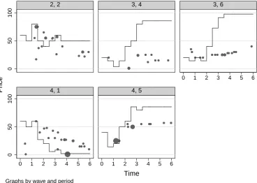
cascade periods in treatment baseline. Figures 2.1 and 2.2 display the according price

patterns separately for each one of the 5 periods that qualify as bad cascade periods.

The first number at the top of each period-specific graph indicates the session while

the second number corresponds to the period. The size of the dots is proportional

to the number of units exchanged. The line corresponds to the expected value of the

asset given all private signals. In treatment sequence, prices clearly fail to converge

to the rational expectations equilibrium in session 3, both in period 4 and period 6.

It could very well be that bad information released early in these periods led to an

information cascade that prevented prices from effectively aggregating information.

However, prices in the corresponding periods of treatment baseline also failed to

converge to the expected value of the asset given all privately held information. As

a result, none of the tests we run allows us to reject the null hypothesis that the

quality of information aggregation in treatment baseline is equivalent to the quality

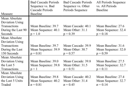
of information aggregation in treatment sequence for bad cascade periods. Table 2.2

contains the p-values of Wilcoxon matched-pairs signed-rank tests for the 4 different

measures of the quality of information aggregation.

Conjecture 2 does not fare much better than conjecture 1. Wilcoxon rank-sum

tests do not allow us to reject the null that the median of the quality of

informa-tion aggregainforma-tion is identical in bad cascade periods compared to other periods within

treatment sequence. When comparing all 35 periods of treatment sequence to all 35

(28)

hypoth-0

50

100

0

50

100

0 1 2 3 4 5 6

0 1 2 3 4 5 6 0 1 2 3 4 5 6

2, 2 3, 4 3, 6

4, 1 4, 5

Price

Time

[image:28.595.140.509.85.347.2]

Graphs by wave and period

Figure 2.1. Prices in Treatment Sequence in Bad Cascade Periods.

esis of equal quality of information aggregation for some of the measures employed

with treatment sequence exhibiting the higher average absolute deviation of prices

from the rational expectations equilibrium price.

The fact that neither one of the main conjectures could be confirmed while there is

some support for the hypothesis that the quality of information aggregation is higher

in treatment baseline compared to treatment sequence might be due to an insufficient

number of bad cascade periods. Clearly, information cascades are not guaranteed to

occur even when the sequence of private signals would provide favorable conditions.

At the same time, information is not always aggregated very efficiently in treatment

(29)

0

50

100

0

50

100

0 .5 1 1.5 2 2.5

0 .5 1 1.5 2 2.5 0 .5 1 1.5 2 2.5

2, 2 3, 4 3, 6

4, 1 4, 5

Price

Time

[image:29.595.141.510.245.501.2]

(30)

[image:30.595.125.537.255.531.2]

Table 2.2. Test Results Bad Cascade Periods.

Measure

Bad Cascade Periods Sequence vs. Bad Cascade Periods Baseline

Bad Cascade Periods Sequence vs. Other Periods Sequence

All Periods Sequence vs. All Periods Baseline

Mean Absolute Deviation Using Transactions During the Last 90 Seconds

Mean Baseline: 39.7 Mean Sequence: 40.1 p = 1.0

Mean Cascade: 40.1 Mean Other: 31.1 p = 0.39

Mean Absolute Deviation Using the Last 5 Transactions

Mean Baseline: 39.0 Mean Sequence: 39.8 p = 1

Mean Absolute Deviation Using the Last 5 Units Traded

(31)

2.4.2 Good Cascade Periods

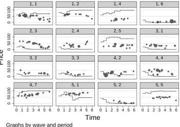
Figures 2.3 and 2.4 display the price patterns in good cascade periods for

treat-ment sequence and treattreat-ment baseline. The size of the dots is proportional to the

number of units exchanged. The line corresponds to the expected value of the

as-set given all private signals. Table 2.3 contains the according test results. We run

Wilcoxon matched-pairs signed-rank tests to obtain the p-values for the first column

and Wilcoxon rank-sum tests for the second column. While only 5 out of 35

peri-ods qualify as bad cascade periperi-ods, 16 qualify as good cascade periperi-ods. This might

be part of the reason why some of the comparisons between treatment sequence and

treatment baseline almost yield significant results. It appears that the quality of

infor-mation aggregation is somewhat lower in good cascade periods in treatment sequence

compared to good cascade periods in treatment baseline.

0

50

100

0

50

100

0

50

100

0

50

100

0 1 2 3 4 5 6 0 1 2 3 4 5 6 0 1 2 3 4 5 6 0 1 2 3 4 5 6

1, 1 1, 2 1, 4 1, 6

2, 3 2, 4 2, 5 3, 1

3, 2 3, 3 4, 2 4, 4

4, 7 5, 1 5, 2 5, 5

Price

Time

[image:31.595.140.511.358.620.2]

(32)

0 50 100 0 50 100 0 50 100 0 50 100

0 .5 1 1.5 2 2.5 0 .5 1 1.5 2 2.5 0 .5 1 1.5 2 2.5 0 .5 1 1.5 2 2.5

1, 1 1, 2 1, 4 1, 6

2, 3 2, 4 2, 5 3, 1

3, 2 3, 3 4, 2 4, 4

4, 7 5, 1 5, 2 5, 5

Price

Time

[image:32.595.138.510.103.360.2]

Figure 2.4. Prices in Treatment Baseline in Good Cascade Periods.

Table 2.3. Test Results Good Cascade Periods.

Measure

Good Cascade Periods Sequence vs. Good Cascade Periods Baseline

Good Cascade Periods Sequence vs. Other Periods Sequence Mean Absolute Deviation

Using Transactions During the Last 90 Seconds

(33)

2.5 Alternative Cascade Period Definitions

2.5.1 Shorter Information Cascades

Clearly, the low number of bad cascade periods combined with a relatively high

vari-ance in the quality of information aggregation in both treatments contributes to the

fact that we did not find much support in favor of conjectures 1 and 2. A possible

remedy would be to apply a more liberal definition of cascade periods by relaxing the

condition that at least 4 out of 8 traders would ignore their private signal if they chose

sequentially whether to buy or sell the asset. However, if only very few traders ignore

their private information, it would be difficult to find significant differences with

re-spect to the quality of information aggregation even if an information cascade actually

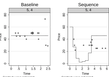
occurred. Therefore, the only extension that we test is one in which at least 3 traders

would ignore their private information if they chose sequentially. Unfortunately, this

more-liberal definition only yields 1 additional bad cascade period (session 5, period

4) and all differences in the quality of information aggregation remain insignificant.

Figure 2.5 displays transaction prices in this additional bad cascade period. The size

of the dots is proportional to the number of units exchanged. The line corresponds

to the expected value of the asset given all private signals.

2.5.2 Who Trades First?

Another reason why conjectures 1 and 2 could not be confirmed might be that the

sequence in which signals are released does not correspond to the sequence in which

subjects actually trade. As a consequence, the sequence in which private information

is revealed to the market might not correspond to the sequence in which signals

are released to traders. To test this hypothesis, we compute the Spearman rank

correlation coefficient between the position of a subject in the sequence in which

private signals are released in treatment sequence and the time at which that subject

first buys or sells at least 1 unit of the asset. We obtain a positive correlation (0.24)

(34)

0

20

40

60

80

0 .5 1 1.5 2 2.5

5, 4

Baseline

Price

Time

0

20

40

60

80

0 1 2 3 4 5 6

5, 4

Sequence

Price

Time

[image:34.595.146.502.101.352.2]

Figure 2.5. Prices in Session 5, Period 4 for Treatments Baseline and Sequence.

Table 2.4. Test Results For Cascade Periods Defined Based on the Time of the First Transaction. We run Wilcoxon rank-sum tests to obtain the p-values.

Measure

Bad Cascade Periods vs. Other Periods Both Treatments

Good Cascade Periods vs. Other Periods Both Treatments

Mean Cascade.: 32.7 Mean Other: 27.4 p = 0.35

(35)

Since the correlation is not perfect, we reclassify cascade periods based on the

sequence in which subjects trade. We apply the same definition of cascade periods

that we originally used (Definition 1) but we now use the sequence of signals obtained

by the first 3 subjects who are buying or selling at least 1 unit of the asset to classify

periods. In treatment sequence, it occasionally happens that some of the these first

3 traders have not yet received their private information at the time at which they

first trade. We are not taking these traders into account since their private signal

clearly cannot have been revealed to the market at such an early stage. As a result,

7 out of 70 periods qualify as bad cascade periods and 5 of these periods are from

treatment sequence and 3 of them were already originally classified as cascade periods.

Wilcoxon rank-sum tests do not allow us to reject the null hypothesis that the median

of the quality of information aggregation in these bad cascade periods differs from the

median in other periods. When redefining good cascade periods based on the time

of the first transaction, 34 out of 70 periods qualify but none of the differences are

significant (table 2.4).

2.5.3 Who Submits Orders First?

Instead of the time of the first transaction, the time at which a trader first submits

a bid or an ask might be more closely related to the time at which he reveals his

private information to the market. Therefore, we test whether the time of the first

bid or ask is related to the time at which the private signal is received in treatment

sequence. The Spearman rank correlation coefficient is 0.29 and we can safely reject

the null that the 2 variables are unrelated (p=0.000). Instead of taking all bids and

asks into account, we only consider bids above 20 and asks below 80 since any signal

would justify lower bids or higher asks.

A reclassification of cascade periods based on the time of the first bid or ask yields

5 bad cascade periods, 4 of these periods already originally qualified as bad cascade

periods. We also obtain 35 good cascade periods. Wilcoxon rank-sum tests do not

(36)

Table 2.5. Test Results for Cascade Periods Defined Based on the Time of the First Order.

Measure

Bad Cascade Periods vs. Other Periods Both Treatments

Good Cascade Periods vs. Other Periods Both Treatments

Mean Cascade.: 31.4 Mean Other: 28.1 p = 0.82

Mean Cascade: 30.2 Mean Sequence: 29.9 p = 0.87

not differ between bad cascade periods and other periods. Good cascade periods also

do not seem to yield a different quality of information aggregation (table 2.5).

2.6 Alternative Explanations

2.6.1 Early Expected Value vs. Late Expected Value

Even though subjects might not completely ignore their private information, they

might place too much weight on information that the actions of other traders reveal.

In that case, misleading early signals would still lead to a lower quality of information

aggregation but not necessarily in such a clear-cut way as the cascade model suggests.

To measure the extent to which early signals are misleading, we compute the expected

value of the asset given the first 4 signals. We then take the absolute value of the

difference between this early expected value and the expected value given all private

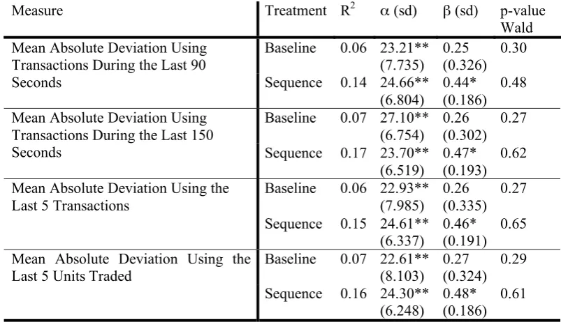
signals. This variable (devalue) is then used to explain the quality of information

(37)

displayed in table 2.6.

In treatment sequence, the coefficient of devalue is always significant at the 10%

level. The larger the difference between the early expected value of the asset and the

late expected value of the asset, the larger the mean absolute deviation of prices from

the late expected value. In that sense, misleading early signals do have an effect on

the extent to which prices converge to the rational expectations equilibrium price.

Since devalue is correlated with the variance of the signals that traders receive,

it could be that a higher variance of signals is the true cause for the observed worse

quality of information aggregation in periods with high values ofdevalue. In that case,

we would expect the coefficient of devalue to be significant in treatment baseline as

well. Since that is not the case, we conclude that the sequence in which signals are

released does indeed affect the extent to which markets can aggregate privately held

information. We also test whether including a variable that measures the standard

deviation of signals significantly improves the fit of these regressions. Wald tests do

not allow us to reject the null hypothesis that the coefficient of the standard deviation

of signals is zero.

2.6.2 Strategic Behavior

When we classify periods as cascade periods, we assume that subjects reveal their

private information to other traders. If they fail to do so, the information that the

market receives might not correspond to the information used to classify periods,

which could explain why information aggregation in bad cascade periods is not

sub-stantially worse than in other periods. In order to test whether subjects are trying to

mislead other traders, we examine the first order submitted in each period. At that

time, the only information subjects have is their private signal. We only consider

bids above 20 and asks below 80 that were made by traders who had already received

their signal. 28% of such first orders are misleading in the sense that subjects are

submitting a buy order even though they received a low signal or that they submit

(38)

in-Table 2.6. Using Devalue to Explain Differences in the Quality of Information Ag-gregation.

Measure Treatment R2 (sd) ! (sd) p-value

Wald Baseline 0.06 23.21**

(7.735) 0.25 (0.326)

0.30 Mean Absolute Deviation Using

Transactions During the Last 90

Seconds Sequence 0.14 24.66**

(6.804)

0.44* (0.186)

0.48

Baseline 0.07 27.10** (6.754)

0.26 (0.302)

0.27 Mean Absolute Deviation Using

Transactions During the Last 150

Seconds Sequence 0.17 23.70**

(6.519)

0.47* (0.193)

0.62

Baseline 0.06 22.93** (7.985)

0.26 (0.335)

0.27 Mean Absolute Deviation Using the

Last 5 Transactions

Sequence 0.15 24.61** (6.337)

0.46* (0.191)

0.65

Baseline 0.07 22.61** (8.103)

0.27 (0.324)

0.29 Mean Absolute Deviation Using the

Last 5 Units Traded

Sequence 0.16 24.30** (6.248)

0.48* (0.186)

0.61

Coefficients marked by (* / **) are significant at the (10 / 5) percent level. Robust standard errors clustered by session are shown in parentheses.

consistent with the private signal received. For example, if a subject received a weak

high signal, the expected value of the asset is 60. It is then perfectly reasonable to

submit a sell order at a price of 70. However, 18% of all first orders are either sell

orders at a price below the expected value given the trader’s private signal or buy

orders at a price above the expected value given the trader’s signal. Clearly, other

traders will find it hard to figure out what signals these traders had based on the bids

or asks that they submitted. No matter whether these are intentional attempts to

mislead other traders or simply mistakes, the fact that bids and asks do not always

reflect the private information that a trader holds makes it difficult do identify the

effect of the sequence of signals on the quality of information aggregation.

2.7 Conclusion

While we find evidence that the sequence in which signals are released to traders

[image:38.595.116.518.112.343.2]

(39)

1 and 2. Bad cascade periods in treatment sequence do not seem to fare substantially

worse than bad cascade periods in treatment baseline or other periods in treatment

sequence. A possible reason could be that we simply do not have enough

observa-tions. Another reason could be the difficulty involved in identifying the sequence in

which information is released to the market. In fact, the sequence in which signals

are released to traders does not always correspond to the sequence in which subjects

actively trade or submit orders. Moreover, when they submit orders, they do not

always reveal their private signal but might instead try to mislead other traders.

An alternative experimental design would eliminate these 2 sources of

complex-ity while still preserving an endogenous price. Instead of allowing subjects to trade

at any point of time, we could require them to trade in a predetermined sequence.

Each subject would be able to submit as many sell and buy orders as desired but

only once. As a consequence, subjects would no longer have an interest in misleading

other traders since it would be impossible to capitalize on flawed prices by

submit-ting further orders at a later point of time. At the same time, the sequence in which

subjects trade would always correspond to the sequence in which they receive their

private information. A control treatment would simply correspond to a call market

with identical signals and value draws. By eliminating much of the complexity of

a continuous double auction while preserving an endogenous price without a

mar-ket maker, such a design should allow us to establish whether information cascades

(40)

Chapter 3 Wise Crowds or Wise Minorities?

This chapter is based on a paper written jointly with Jacob K. Goeree.

3.1 Introduction

When people are imperfectly informed they may try to learn from others’ choices.

Prospective graduate students, for instance, often inquire which schools other students

chose to apply to. Teenagers consult the charts before deciding which CD to buy and

tourists tend to prefer well-occupied restaurants to half-empty competitors. In many

of these situations, only others’ choices can be observed, not the exact information

they had when making their choices. And while in some instances the exact sequence

of predecessors’ choices is observed (as in the US primary elections), more often only

aggregate statistics based on those choices are available (e.g., the number of diners

in a restaurant).

When do others’ decisions contain relevant information and what course of action

do they suggest? Obviously, predecessors’ choices matter only when their payoffs are

correlated to some extent. For this reason, most of the social-learning literature makes

the simplifying assumption that agents have identical values for the available options,

as is the case, for instance, when buying stocks.1 _{In this common-value environment,}

(41)

folk wisdom suggests it would be best to follow the majority, an intuition that is

formalized by theoretical models of social learning. Bikhchandani et al. (1992), for

example, consider a model where agents are privately informed about which of 2

options is better and the quality of information is the same across agents. They

demonstrate that after a few decisions, information cascades occur and all agents

herd on the majority choice regardless of their private information.2 Following the

majority is also optimal in Banerjee’s (1992) model where uninformed agents have

the ability to signal that they have no information.

In contrast, Callander and H¨orner (2009) consider a situation where it can be

optimal to follow the minority. In their model, agents differ in terms of the quality

of information they possess and observe only the number of decisions for each option.

In this paper, we consider the following simplified version of their model: each agent

has a small chance of being perfectly informed about which of 2 options is correct or

gets no information at all (besides the prior information that puts equal weight on

both options). The information agents receive and the order in which they move are

exogenously determined.3 Finally, the probability of being informed is low enough

such that, under common knowledge of rationality, it is always optimal to follow the

minority. This result is explained in more detail below, but to glean some intuition

consider an uninformed agent who learns that 2 predecessors have chosen restaurant

A and one has chosen restaurant B. Such an outcome can only occur when the first agent was uninformed and chose the worse of the 2 restaurants. If both the second

and the third agent were informed, it would be best to follow the majority but such a

case is relatively unlikely when the probability of being informed is low. When only

the second agent was informed, the third agent faces a tie and chooses randomly, in

which case following the minority is no worse than following the majority. As opposed

where predecessors’ choices affect payoffs by changing the prices of the alternatives.

2_{Laboratory evidence provides partial support for these predictions in the sense that information} cascades do occur but are often broken. In addition, subjects tend to overweigh their private information vis-`a-vis that contained in publicly observable predecessors’ choices (see, e.g., Anderson and Holt, 1997; C¸ elen and Kariv, 2004a, 2004b; Goeree et al., 2006, 2007).

(42)

to a sequence with 2 informed agents, it is quite likely that only the third agent was

informed, in which case it is strictly better to follow the minority.

This simple logic extends to more general minority-majority divisions if common

knowledge of rationality can be subsumed (see Callander and H¨orner, 2009). But

once we introduce the possibility of “trembles” or mistakes, it breaks down. Goeree

et al. (2007), for example, find that in standard social learning experiments (based

on Bikhchandani et al., 1992), cascades do form but almost never last as subjects

frequently opt to follow their contrary information and break the cascade.4 While

un-informed agents in our experiment do not possess any private information,5 _trembles

may still occur especially because the information conveyed by predecessors’ choices

may be of low quality and value. Intuitively, the possibility of trembles greatly alters

equilibrium predictions in the Callander–H¨orner setup. In the example above, for

instance, the 2–1 division between restaurants is more likely caused by a trembling

uninformed agent than by a deviating informed agent when the probability of being

informed is very low.

More generally, whether it is optimal to follow the majority or the “deviant

minor-ity” therefore depends on the likelihood of mistakes, the quality of others’ information,

the correlation of tastes, etc. It would be hard to distinguish these confounding

ele-ments in data from the field, which is why we turn to the lab. We conducted 2 types

of sequential decision-making experiments: in treatment “sequence,” agents can see

the entire sequence of predecessors’ decisions and in treatment “no-sequence” they

only see the number of predecessors’ choices for either option. Collecting data from

both treatments allows us to connect our findings to prior literature, which mostly

employs the sequence treatment, and enables us to evaluate the efficiency gains that

may result from the additional information in treatment sequence.

4_{In these experiments, cascade breaks are informative and prevent the learning process from} getting stuck. As a result, full information aggregation becomes possible in the limit as the number of agents grows large. Goeree et al. (2007) demonstrate how a logit quantal response model can account for much of the dynamics in the experiments.

(43)

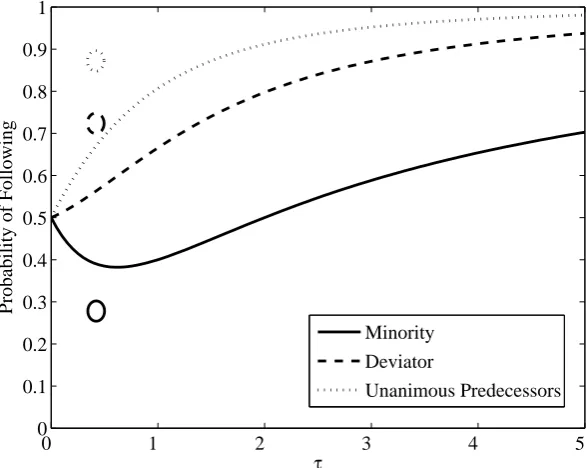
We find that informed subjects always follow their signal, i.e., they always pick

the correct option. On average, uninformed subjects tend to follow unanimous

pre-decessors close to 90% of the time both in treatments sequence and no-sequence.

Furthermore, the frequency with which unanimous predecessors are followed

signifi-cantly rises (to levels between 90% and 100%) as the number of predecessors grows.

This high percentage of rational choices is maybe not surprising given that the

deci-sion problem faced by an uninformed agent is relatively easy when all predecessors

agree. When there is a deviator in treatment sequence, subjects tend to follow the

deviator only 72% of the time. The frequency with which a deviator is followed is

significantly higher when the deviator’s choice belongs to the majority (80%) than

when it belongs to the minority of previous choices (58%). Finally, in treatment

no-sequence, subjects tend to follow the minority only 28% of the time. This

percent-age significantly declines when the difference between the number of majority and

minority choices grows.

While observed choices deviate from theoretical predictions, they are approximate

best responses to the empirical distribution of play in the following sense. Given

the choices of others, and given the signals used in the experiment, the cost of not

following unanimous predecessors in the experiment is $1.53 on average. Likewise, the

cost of not following a deviator in treatment sequence is $1.23 on average, and the cost

of not following the minority is −$0.36 on average. In other words, subjects who are (imperfect) profit maximizers would nearly always follow unanimous predecessors,

would more likely than not follow a deviator in treatment sequence (although not

as frequently as they would follow unanimous predecessors), and would follow the

majority in treatment no-sequence. The canonical model that captures this type of

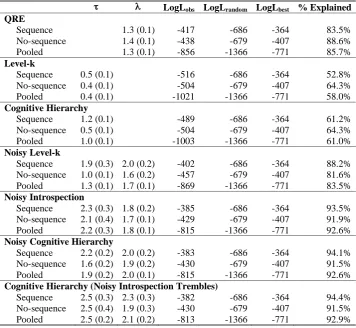
imperfect maximization behavior is the (logit) QRE model. We show that, on an

aggregate level, logit-QRE is able to reproduce the main features of our data quite

well.

In the logit-QRE model, however, agents are assumed to be ex ante symmetric,

which is clearly not true in our data. While some subjects make rational choice in all

(44)

heterogeneity is captured by models that allow for different levels of strategic thinking,

such as the level-k model (e.g., Crawford and Iriberri 2007a, 2007b) and cognitive hierarchy (Camerer, et al. 2004). When we apply level-k and cognitive hierarchy to the data, we find they produce a worse fit both on an individual and aggregate level.

The reason for their poor performance is that these models subsume best response

behavior (given beliefs), except for level-0 who randomizes when uninformed. The

best-response assumption often conflicts with intuitive comparative statics observed

in the data, e.g., subjects tend to follow unanimous predecessors more frequently

when the group of predecessors is large. In addition, the best-response assumption

implies that a subject who mostly but not always makes a rational choice, is classified

as level-0 even though most of her choices suggest a higher level of thinking.

Goeree and Holt (2004) propose a “noisy introspection” model that blends the idea

of different levels of strategic thinking with noisy responses (trembling). In particular,

the noisy introspection model replaces the strict best responses of the level-k model with logit “better responses.” Importantly, agents in the noisy introspection model

are assumed to be aware that others tremble. For example, when computing the

probability that the minority choice is correct in treatment no-sequence, agents take

into account the possibility that the minority arose because of trembles. As a result,

the model can predict why subsequent choices favor the majority (not the minority)

even for agents with high levels of strategic thinking.

We find that the noisy introspection model provides a significant improvement in

fit relative to logit-QRE and a dramatic improvement relative to level-k and cogni-tive hierarchy. To illustrate the importance of the “common-knowledge-of-trembling”

assumption that underlies noisy introspection, we also estimate a noisy version of

the level-k model in which agents tremble but assume others do not. We find that the noisy level-k model provides a better fit than level-k and cognitive hierarchy, but does not do nearly as well as noisy introspection. We also estimate 2 versions of the

cognitive hierarchy model with trembles, one in which agents are aware that others

tremble and one in which they are not. Both of these models fit the data equally well

(45)

The chapter is organized as follows. In the next section, we briefly discuss the

theoretical predictions for the 2 treatments. The experimental design is presented in

section 3.3. The results of the experiment can be found in section 3.4. In section

3.5, we apply alternative models of bounded rationality to explain individual and

aggregate outcomes. Section 3.6 concludes.

3.2 Theoretical Predictions

Treatment sequence is a simple variant of the social learning model proposed by

Bikhchandani et al. (1992). There are 2 options, A and B, that are equally likely to be correct and a finite set ofnagents labeledt= 1,2, . . . , n. Each agent chooses either A or B after having observed a private signal st and the decisions of predecessors. Signals in the experiment are either fully informative or not informative at all: if

ω denotes the correct option then st = ω with probability q > 0 and st = ∅ with probability 1−q.

Given that some agents may be fully informed, the perfect Bayesian equilibria of

sequence treatment are easy to derive. First, an agent withst=ωchoosesω. Second, if all predecessors agree, then an uninformed agent follows the majority since either all

predecessors were uninformed and the agent is indifferent or some predecessors were

informed and the agent strictly prefers to follow the majority. Third, if predecessors

were not unanimous, i.e. choices switched from one option to the other, then the

first predecessor who “deviated” by not following her predecessors must have been

informed. In this case, the agent should follow the deviator. Note that all 3 cases can

be succinctly summarized as follows: under common knowledge of rationality,

unin-formed agents follow their immediate predecessor. Finally, if predecessors switched

from one option to the other and then switched back, play is off the equilibrium path.

In this case, the agent cannot infer anything from prior play and simply randomizes

when st=∅ and chooses ω when st =ω.

Information Aggregation and Allocative Efficiency in Complex Environments

in Complex Environments

Christoph Brunner

Acknowledgements

Abstract

Contents

List of Figures

List of Tables

Chapter 1

Introduction

Chapter 2

Cascades in Experimental Asset

Markets

2.1

Introduction

2.2

Experimental Design

2.3

Conjectures and Definitions

2.4

Results

2.4.1

Bad Cascade Periods

2.4.2

Good Cascade Periods

Price

Time

Price

Time

2.5

Alternative Cascade Period Definitions

2.5.1

Shorter Information Cascades

2.5.2

Who Trades First?

Baseline

Sequence

2.5.3

Who Submits Orders First?

2.6

Alternative Explanations

2.6.1

Early Expected Value vs. Late Expected Value

2.6.2

Strategic Behavior

2.7

Conclusion

Chapter 3

Wise Crowds or Wise Minorities?

3.1

Introduction

3.2

Theoretical Predictions