Old dog, new tricks: a modelling view of simple moving averages
Ivan Svetunkova, Fotios Petropoulosb,∗
aCentre for Marketing Analytics and Forecasting, Lancaster University Management School, UK bSchool of Management, University of Bath, UK
Abstract
Simple moving average (SMA) is a well-known forecasting method. It is easy to understand and interpret and easy to use, but it does not have an appropriate length selection mechanism and does not have an underlying statistical model. In this paper we show two statistical models underlying SMA and demonstrate that the automatic selection of the optimal length of the model can easily be done using this finding. We then evaluate the proposed model on a real dataset and compare its performance with other popular simple forecasting methods. We find that SMA performs better both in terms of point forecasts and prediction intervals in cases of normal and cumulative values.
Keywords: Forecasting, modelling, state-space models, Simple Moving Average, ARIMA
1. Introduction
Simple moving average (SMA) is a very basic forecasting method, that is widely used in practice, sometimes competing with exponential smoothing, usually ending up being the second popular in companies (for example, see Winklhofer, Diamantopoulos, and Witt, 1996; Weller and Crone, 2012). The reason for its popularity is the simplicity of the method – practitioners can understand what it implies and how it can be used. However, being a simple method, it has several drawbacks. First, the order (length) of moving average needs to be selected before applying the method. This is usually done using forecaster’s judgment. Second, there is no concise statistical model underlying the SMA. This makes the construction of the correct parametric prediction intervals close to impossible, which in practice leads to challenges in inventory control decisions. Third, because of its simplicity the SMA does not seem interesting to academics. As a result, the SMA is usually neglected in forecasting research and is not considered as a forecasting method worth investigating.
In this paper we demonstrate two simple statistical models underlying the SMA. This finding allows looking at the SMA from a new perspective making it a sophisticated model.
∗Correspondence: Fotios Petropoulos, School of Management, University of Bath, Claverton Down, Bath,
BA2 7AY, UK.
Email addresses: [email protected](Ivan Svetunkov),[email protected]
This also allows automating order selection for the SMA and constructing the correct predic-tion intervals. We show that using the SMA in this new form simplifies forecasting process and demonstrate on the example of real data the advantages of the SMA in comparison to several other basic forecasting models.
2. Literature Review
Over the years the Simple Moving Average was mainly discussed in inventory control context. It is usually considered as one of the competitors of Simple Exponential Smooth-ing (SES) and is used very often for cases of low level and intermittent data mainly as a benchmark (see, for example Syntetos and Boylan, 2006; Rego and Mesquita, 2015).
Sani and Kingsman (1997) compare several forecasting methods in terms of inventory performance on simulated data. They find that the SMA(12) performs very well for the low level data, outperforming the SES with a non-optimised smoothing parameter.
Syntetos and Boylan (2006) compare the SES, the SMA(13) and two other forecasting methods on both simulated and real intermittent data. They assess the performance of the methods on customer service level and find that the SMA(13) is one of the best forecasting methods in the comparison.
Ali and Boylan (2012) discuss the prevalence of the SMA and the SES in practice. They also show how the variance of the demand influences the supply chain when the SMA and the SES are used instead of the correct ARIMA model for forecasting purposes. In a follow-up paper, Ali et al. (2015) discuss the advantages of the SMA for downstream demand inference when the information about the demand is not shared in the supply chain.
As it can be seen, the SMA is used in inventory management literature as a method for different purposes, but has not been studied on its own. The similar situation is in the forecasting context, where the SMA is discussed even less often, and is seldom included as a benchmark. For example, it was included in the original M-competition (Makridakis et al., 1982), where the authors selected the optimal length of the SMA based on the minimum of sum of squared errors. The authors showed that the SMA with order selection performed very similar to the SES (measuring the accuracy using MAPE – Mean Absolute Percentage Error), slightly outperforming SES on monthly data. The difference in performance of the two methods seems statistically insignificant, but have never been explored in detail. However, it was excluded from the follow-up M3-competition (Makridakis and Hibon, 2000). The only attempt to develop a statistical model underlying the SMA was given by John-ston et al. (1999). The authors discuss the SMA and the SES and show that the SMA can be connected to a steady-state model, but do not discuss this model in details, focusing on variances calculations. The authors derive conditional variance for the SMA and the variance for the level. They also derive the formula for the optimal SMA length calculation, which minimises variance of the level of the model. Finally, based on these results, they derive the formula, connecting smoothing parameter α of the SES and the length of the SMA:
k =
r
2(1−α)
α2 +
1
wherekis the order (length) of the SMA andα is the smoothing parameter of the SES. The same formula can be rewritten as:
α=
√
12k2 + 3−3
2k2−1 . (2)
However, these two formulae can only demonstrate an approximate connection between the SES and the SMA, because of the fundamental differences between the two methods: the former is based on the infinite weighted average of the actual values, while the latter is based on the fixed order of uniformly-weighted average of the k actual values. Furthermore,k = 1 for the SMA corresponds in (2) to α≈0.87, although both methods should revert to Na¨ıve method in this case, taking only one, recent observation as a forecast (meaning that α= 1 in the SES). This shows that the derived formula (2) is approximate and can only give a general understanding of how the two methods can be connected.
Johnston et al. (1999) conduct the simulation experiment, but never evaluate the per-formance of the SMA on the real data.
Overall, the question of the statistical model underlying the SMA was neglected in the literature over the years. There are several reasons for that. This topic is not considered as an interesting one for academics, because the SMA is perceived as a simple forecasting method. Despite the ample evidence that simple models perform on average as good as more complicated ones (see for example Makridakis et al., 1982; Makridakis and Hibon, 2000), still some academics focus on deriving and proposing complicated, statistically sophisticated and more challenging models rather than on studying the properties of the simpler ones. Fur-thermore, most of the widely-used commercial forecasting software provide relatively simple methods that have shown to perform well. Taking all of these into account, deriving statis-tical models underlying the SMA and studying their properties should benefit both sides: practitioners who use this method and academics who neglect it because of its simplicity.
3. Models Underlying SMA
The basic formula for the SMA can be written as:
ˆ
yt=
1
k
k
X
i=1
yt−i, (3)
where yt is an actual value, ˆyt is a forecast for the observation t and k is the length of
the SMA. In order to derive a statistical model underlying (3), the error term needs to be introduced. The simplest way to do that is to say thatyt= ˆyt+t, wheret ∼ N(0, σ2). Then
a simple model underlying the forecasting method (3) can be formulated in the following way:
yt=
1
k
k
X
i=1
If the actual values are moved to the left hand side of the equation (4), then we end up with:
yt−
1
k
k
X
i=1
yt−i =t, (5)
which is AR(k) process, that can be written in the following compact form:
1−
k
X
i=1
φiBi
!
yt =t, (6)
where all φi =φ = 1k and Pki=1φi = 1. As we see, any SMA method has underlying AR(k)
model. Knowing that, allows looking differently at the usage of this forecasting method. First inference that can be made based on (6) is that the condition Pk
i=1φi = 1 means
that any AR(k) model underlying SMA(k) is not stationary, because at least one of the roots of the polynomial will always be equal to one, meaning that it lies on the unit circle edge. This can be seen by analysing the the characteristic equation 1−Pk
i=1φixi = 0, for which
x= 1 is one of the roots. This property of the SMA shows its similarity to the SES, which has an underlying non-stationary ARIMA(0,1,1) model.
Second, in case ofk = 1, the SMA model corresponds to the Random Walk, while in the case of k → ∞ it corresponds to a model with the global (deterministic) level. This means that in general the SMA model can be applied to a wide variety of level time series with different characteristics.
Third, initialisation of AR(k) model can be done in different ways, some of which would allow preserving observations, so the problem of losing k observations at the start of time series can now be resolved. This can be done, for example, using backcasting or Kalman filter.
Fourth, statistical model allows selecting the most appropriate order k for time series using information criteria, so the selection of the SMA length becomes no longer an issue. Notably, there are only two parameters to estimate in the SMA of any length: the value ofφ
and the variance of error term. This means that the Mean Squared Error, lying in the core of likelihood method (assuming normal distribution), determines the correct order, given that the sample sizes of all the SMA models are the same. This finding indirectly supports the approach used by Makridakis et al. (1982). An example of information criterion used for optimal order selection is AIC (Akaike’s Information Criterion):
AIC = 2·2−2`(θ|Y), (7)
Fifth, a correct conditional mean can be produced using this statistical model, which is not necessarily a straight line, but will always be something converging to a constant. This means that eventually any SMA model will produce a straight line as a point forecast, but it may take some time to converge to that value depending on the length k. This feature corresponds to the one in AR models.
Finally, using (6), a conditional variance can be calculated, which allows producing the correct parametric prediction intervals for any SMA.
Knowing (6) also allows deriving state-space models underlying any SMA, which sim-plifies the derivation of conditional variance of the model and potentially allows treating missing values on the fly. This can be done either in Multiple Source of Error (Durbin and Koopman, 2012) or in Single Source of Error (Snyder, 1985) framework. For example, the latter can be written as the following system (using Hyndman et al., 2008, p.174):
yt =w0vt−1+t
vt =Fvt−1+gt
, (8) where F= 1
k In−1
.. . 1 k 0 ,g=
1 k .. . 1 k ,w=
1 0 .. . 0 ,
and vt is the vector of states. The initial values of vt can be estimated via maximisation of
likelihood function, but for short lengths of SMA this will result in overfitting of the firstk
observations of data, which in a way leads to the loss of thesek observations. So in order to preserve them, we propose using backcasting. This procedure is done iteratively. On each iteration the following is done:
1. The model (8) is fitted to the data from the first observation till the last one;
2. When the end of the data is reached, the following equation is used in order to recal-culate the states values and obtain new estimates of the initial state vector:
yt=w0vt+1+t
vt=Fvt+1+gt
. (9)
This equation is used from the last observation till the very first one. The new initial state v0 is obtained.
This procedure is repeated several times until the stable estimate of initials state v0 is obtained.
The conditional variance of the state-space model (8) has been discussed in (Hyndman et al., 2008), but the model also allows deriving the cumulative conditional variance, which corresponds to the aggregated over the forecasting horizon estimate (see Appendix A for the derivation):
σ2c,h =σ2 1 +
h−1 X
j=1
1 + (h−j)w0Fj−1g2
!
, (10)
whereσ2 is the variance of one-step-ahead forecast error,h is the forecast horizon andσ2
c,h is
the conditional cumulative variance (conditional on the values available on the observation
t). The variance (10) can be used for safety stock calculations in an inventory control system.
4. Experimental design
In order to see how the proposed model performs in practice, we conduct an experiment on real data.
4.1. Dataset
We use real monthly sales data coming from a multinational pharmaceutical company. The data span over a period of 25 months, and it has been used before to examine the performance of statistical and judgmental forecasts (see for example Franses and Legerstee, 2009, 2011; Petropoulos, Fildes, and Goodwin, 2016; Wang and Petropoulos, 2016). In this paper, we only use the actual values from the dataset.
The complete dataset consists of 1101 time series, however, we filtered out series which contained invalid data points. Furthermore, as the proposed forecasting model is a level one, we are focusing on the level time series. This was tested using ADF and KPSS tests (kpss.test() and adf.test() functions from tseries package in R); a time series was flagged as level if either the null hypothesis was not rejected in KPSS or the null hypothesis was rejected in ADF. Taking that the sample size for each time series is small (25 observa-tions), we ended up having both global and local level series, which added up to 664 time series.
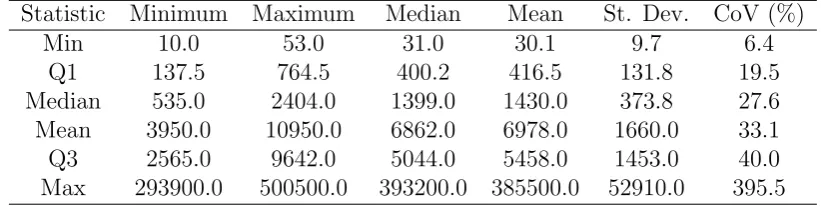
The descriptive statistics of the data are presented in table 1. The various statistics that are calculated within the series are presented in columns (minimum, maximum, median, mean, standard deviation and coefficient of variation), while the rows present the six-figure summary (minimum, first quartile, median, mean, third quartile and maximum value) across all series.
4.2. Benchmark models used in the evaluation
We use the following popular level models as benchmarks in order to assess the perfor-mance of SMA:
1. Random walk, which has Na¨ıve as forecasting method (denoted as “Na¨ıve” in this paper):
Table 1: Descriptive statistics (columns) of the data used, calculated per series and analysed across series (rows).
Statistic Minimum Maximum Median Mean St. Dev. CoV (%)
Min 10.0 53.0 31.0 30.1 9.7 6.4
Q1 137.5 764.5 400.2 416.5 131.8 19.5
Median 535.0 2404.0 1399.0 1430.0 373.8 27.6
Mean 3950.0 10950.0 6862.0 6978.0 1660.0 33.1
Q3 2565.0 9642.0 5044.0 5458.0 1453.0 40.0
Max 293900.0 500500.0 393200.0 385500.0 52910.0 395.5
It is worth noting that Random Walk model can be represented as ARIMA(0,1,0) model:
(1−B)yt =t. (12)
This is the simplest forecasting model and it is used mainly as a benchmark for all the other models. We do not expect this forecasting method to perform very well in our experiment, because the data seems to be well behaved, while Naive has a short memory, taking only last observation into account.
2. Average of the whole series (denoted as “Average”):
yt=l+t, (13)
wherelis the average level of the whole series. This model is expected to perform bet-ter on our dataset than Na¨ve, because it has long memory, taking all the observations into account. However we do not know how it will perform against other competi-tors. Following the derivations similar to SMA, it can be shown that Average has ARIMA(n,0,0) model, where n is the number of in-sample observations:
1− 1
nB −
1
nB
2− · · · − 1
nB
n
yt =t. (14)
3. ETS(A,N,N), which underlies Simple Exponential Smoothing method (denoted as “SES”):
yt =lt−1+t
lt=lt−1+αt
, (15)
where lt is level component and α is smoothing parameter. This is one of the most
popular forecasting models used in inventory control and it is the main competitor of the SMA. This model can also be represented as ARIMA(0,1,1) model:
(1−B)yt= (1 +θ1B)t, (16)
4. AR(p) model:
1−φ1B−φ2B2− · · · −φpBp
yt=t, (17)
where φji is the i-th parameter. This model is added as it can be considered an
unrestricted version of SMA, model that allows arbitrary weights distribution over the observations. The estimation of the model can be done using OLS, while the selection of the optimal orderpis done using an information criterion. This is the most flexible model of all the models included in our competition, so potentially it can outperform the others.
We use smooth package for R (v2.1.1, available on CRAN) for all of these models. In order to assess the performance of the SMA, we use the function sma(), which imple-ments the model in the state-space form (8) with automatic order selection and is called the following way: sma(y, ...). We also use es() function for the SES, the Na¨ıve and the Average. The SES is applied with optimal smoothing parameter to each separate time series and forecast origin and is called using: es(y, model="ANN", ...). For the Na¨ıve, we set the smoothing parameter of the SES equal to one: es(y, model="ANN", persistence=1, ...). For the Average we set the initial level of the SES equal to the av-erage of the in-sample data and smoothing parameter equal to zero: es(y, model="ANN", persistence=0, initial=mean(y), ...). Finally, for the AR(p) model we useauto.ssarima()
function, which implements ARIMA in state-space form and allows selecting the optimal order based on an information criterion, with a restriction on the maximum autoregres-sive order of the model equal to the minimum in-sample size (15 periods). The following call is used for that: auto.ssarima(y, orders=list(ar=15), lags=1, constant=FALSE, workFast=FALSE, initial="backcasting", ...).
For each of the models we produce both point forecasts and prediction intervals of 80% and 95% width. We produce both simple and cumulative values for both point forecasts and prediction intervals (this is regulated by the booleancumulative parameter). The former is needed in order to assess the models from forecasting perspective, while the latter is useful as it directly links with inventory control systems.
4.3. Measures
We consider a range of error measures to evaluate the performance of the point forecasts of the SMA model against that of the benchmark models. First, we consider two percentage accuracy measures, namely the Mean Absolute Percentage Error (MAPE) and the symmetric Mean Absolute Percentage Error (sMAPE). While we acknowledge the disadvantages of these error measures (see for example Goodwin and Lawton, 1999; Hyndman and Koehler, 2006), we believe that their inclusion is necessary given their popularity in practice.
Error (sMAE) and the scaled Mean Squared Error (sMSE). These were used by Petropoulos and Kourentzes (2015), while Kolassa (2016) discussed the advantages of sMSE over other measures in the context of intermittent demand. The scaling of sME and sMAE is performed by the arithmetic mean of the in-sample data, while the scaling of sMSE is done by the square of the arithmetic mean of the in-sample. sME is appropriate for measuring the bias of the forecasts, sMAE (similarly to MASE) measures accuracy, while sMSE additionally to the bias provides insights on the variance of the forecast errors.
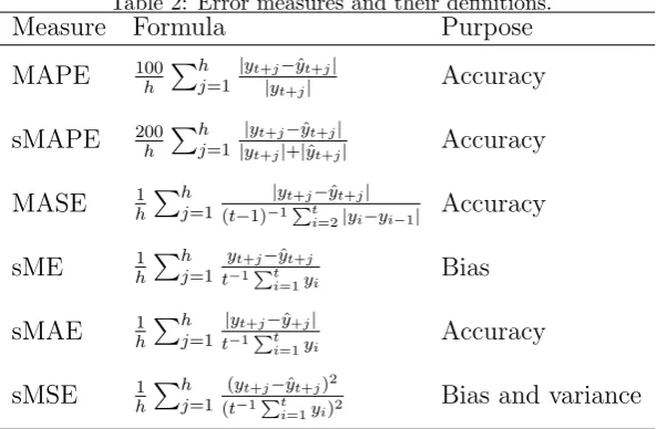
Table 2 presents the definitions of the six error measures used in this study. We denote the size of the in-sample with t, yt is the actual value at period t, yt+h and ˆyt+h are the
[image:9.595.148.445.281.475.2]actual and the forecast h periods ahead, and h is the forecast horizon.
Table 2: Error measures and their definitions.
Measure Formula Purpose
MAPE 100h Ph
j=1
|yt+j−yˆt+j|
|yt+j| Accuracy
sMAPE 200h Ph j=1
|yt+j−yˆt+j|
|yt+j|+|yˆt+j| Accuracy
MASE 1hPhj=1 |yt+j−yˆt+j|
(t−1)−1Pt
i=2|yi−yi−1| Accuracy sME 1hPhj=1 yt+j−ˆyt+j
t−1Pt
i=1yi Bias
sMAE 1hPh
j=1
|yt+j−yˆ+j|
t−1Pt
i=1yi Accuracy
sMSE 1hPh
j=1
(yt+j−yˆt+j)2
(t−1Pt
i=1yi)2 Bias and variance
In addition to the error measures for evaluating the performance of point forecasts, we consider three measures to assess the prediction intervals produced by each model:
• Coverage, which refers to the percentage of times where the actuals do not lie outside the lower and upper bounds of the prediction intervals.
• Upper coverage, which refers to the percentage of times where the actuals do not surpass the upper bound of the prediction intervals. We use this measure as a proxy for the fill rate of demand, where the targeted service level (SL) is linked to the confidence level of prediction intervals (CL) as: CL= 2·SL−1.
• Spread of the prediction intervals, calculated as the difference between upper and lower bounds of the prediction interval divided by the mean of the in-sample data. We use this measure as a proxy for the inventory holding cost, as the spread of the prediction intervals can be associated with the calculation of the safety stock.
4.4. Process
of each model and then produce forecasts for the next three periods (16, 17 and 18); in other words, we set the forecast horizon to three periods ahead. A forecast horizon of three periods ahead allows us to explore the performance of the models for more than one steps ahead and to evaluate models across multiple origins. Subsequently, the performance of each model is measured using the metrics defined in Subsection 4.3 by comparing the forecasts for the periods 16 to 18 with the respective actual observations.
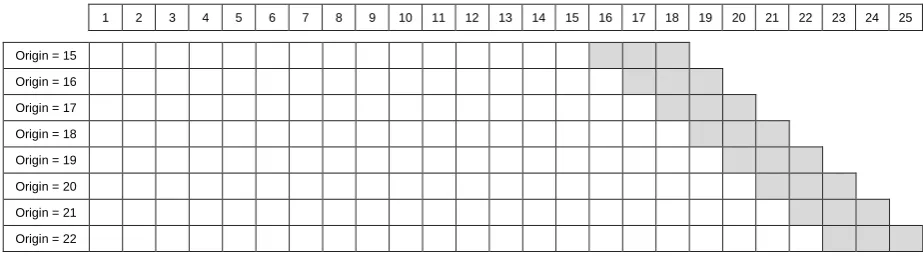
[image:10.595.66.528.329.458.2]We then increase the in-sample set by one observation, setting the forecast origin to period 16. Parameters are re-estimated, forecasts are produced for the required horizon (periods 17, 18 and 19) and performance is measured. The process continues by rolling through the data, period after period, till we reach the end of the data. The last forecast origin is period 22, from which we produce forecasts for periods 23 to 25. All in all, we produce three-steps-ahead forecasts 8 times (from origins 15 to 22).
Figure 1 provides a visual representation of the evaluation process applied for this study. This process is repeated for each of the 664 time series.
1 2 3 4 5 6 7 8 9 10 11 12 13 14 15 16 17 18 19 20 21 22 23 24 25
Origin = 15
Origin = 16
Origin = 17
Origin = 18
Origin = 19
Origin = 20
Origin = 21
Origin = 22
Figure 1: The rolling process applied for evaluating the performance of the SMA model.
White cells in Figure 1 correspond to the training set of data, while the grey cells correspond to the test part. All the models were estimated on the former part and assessed on the latter one.
5. Empirical results
5.1. Evaluation of point forecasts
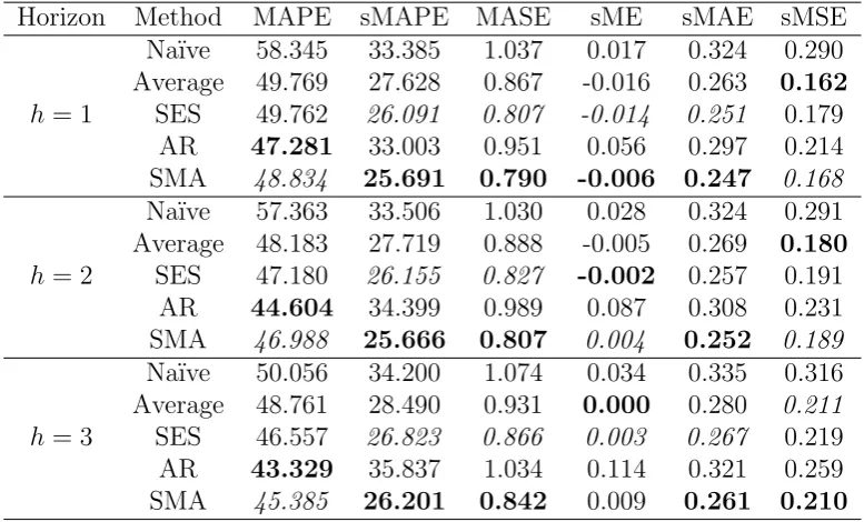
Table 3 presents the performance of the Na¨ıve, the Average, the SES, the AR and the SMA for the various error measures defined in Subsection 4.3 and for different horizons (1 to 3 steps ahead). The performance of each model has been averaged (arithmetic mean) across eight validation samples (see figure 1) and 664 time series. The best and second-best performances across the methods for each error measure are presented in boldface and italic respectively.
Table 3: Point forecast performance of the SMA against the Na¨ıve, the Average, the SES and the AR for the various error measures and different forecasting horizons.
Horizon Method MAPE sMAPE MASE sME sMAE sMSE
h= 1
Na¨ıve 58.345 33.385 1.037 0.017 0.324 0.290
Average 49.769 27.628 0.867 -0.016 0.263 0.162
SES 49.762 26.091 0.807 -0.014 0.251 0.179
AR 47.281 33.003 0.951 0.056 0.297 0.214
SMA 48.834 25.691 0.790 -0.006 0.247 0.168
h= 2
Na¨ıve 57.363 33.506 1.030 0.028 0.324 0.291
Average 48.183 27.719 0.888 -0.005 0.269 0.180
SES 47.180 26.155 0.827 -0.002 0.257 0.191
AR 44.604 34.399 0.989 0.087 0.308 0.231
SMA 46.988 25.666 0.807 0.004 0.252 0.189
h= 3
Na¨ıve 50.056 34.200 1.074 0.034 0.335 0.316
Average 48.761 28.490 0.931 0.000 0.280 0.211
SES 46.557 26.823 0.866 0.003 0.267 0.219
AR 43.329 35.837 1.034 0.114 0.321 0.259
SMA 45.385 26.201 0.842 0.009 0.261 0.210
good performance of AR in terms of MAPE is not confirmed when other measures are considered. It is noteworthy that AR produces the most biased forecasts based on sME. Also, as we expected, the Na¨ıve performs overall the worst, a result that is consistent across all accuracy measures. The good performance of the SMA can be explained by the fact that we dealt with the data with slowly changing level in this dataset. As a result, taking the average of several last observations allows capturing the level better than distributing weights in an exponential manner (SES) or taking all the observations into account (as Average model does).
Note that the SMA outperforms the SES in all measures apart from sME for horizons 2 and 3 steps ahead. This is a very important finding, especially if we consider the popularity of the latter and its widespread application across the industry. Our finding is also consistent with the “simple rather than complex” agenda in forecasting (Makridakis and Hibon, 2000). Being in position to estimate the optimal order (k) per series and origin, the SMA model achieves not just similar but better performance than the SES, with a simpler estimation process. Fitting an optimal SMA model requires, apart from the variance of the errors, the estimation of a single parameter (k) in contrast to the SES where the same process implies the estimation of two parameters (the smoothing parameterα and the initial level l0).
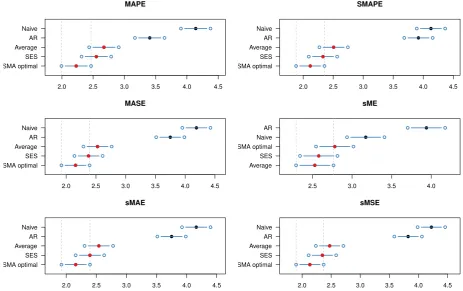
of the value of order, k) achieves the best average rank performance among the five models for five out of six measures. However, while the Na¨ıve and AR perform significantly worse than the other three models, the SMA performs similar to the Average and the SES, as indicated by the overlapping rank intervals.
MAPE
SMA optimal SES Average AR Naive
2.0 2.5 3.0 3.5 4.0 4.5
SMAPE
SMA optimal SES Average AR Naive
2.0 2.5 3.0 3.5 4.0 4.5
MASE
SMA optimal SES Average AR Naive
2.0 2.5 3.0 3.5 4.0 4.5
sME
Average SES SMA optimal Naive AR
2.5 3.0 3.5 4.0
sMAE
SMA optimal SES Average AR Naive
2.0 2.5 3.0 3.5 4.0 4.5
sMSE
SMA optimal SES Average AR Naive
[image:12.595.65.529.194.485.2]2.0 2.5 3.0 3.5 4.0 4.5
Figure 2: Multiple Comparisons from the Best test for SMA and benchmark models.
In order to investigate further the performance of the SMA, we analyse the selected optimal orders by the model. Figure 3 presents the histogram of these orders (the total number of fitted models is 664 time series × 8 origins). While we observe a great variation with regards to the optimal value of order k, we also observe concentrations around the values 12 to 16. This may indicate that the time series under consideration do not exhibit rapid changes in level, because the moving average of one year of data and more is used very often. This also aligns with findings of Sani and Kingsman (1997); Syntetos and Boylan (2006), where the SMA(12) and the SMA(13) performed very well in real time series. Figure 3 also provides an indication of the flexibility of the SMA model towards the selection of different values ofk as the series evolve.
1 3 5 7 9 11 13 15 17 19 21
Order
Frequency
0
100
300
[image:13.595.155.433.112.255.2]500
Figure 3: Frequency of the selected optimal orders (k).
when the smallest possible sample is considered (origin 15). We denote each fixed SMA model as SMA(k). Note that the SMA(1) is equivalent to the random walk model.
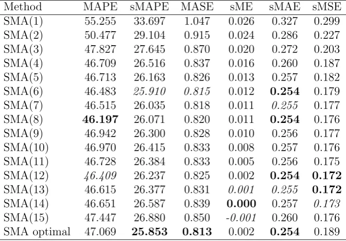
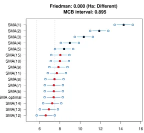
[image:13.595.118.474.445.693.2]Table 4 presents the performance of the optimal versus the fixed-order SMA models for the various error measures considered. The proposed optimal SMA model have the best average performance for three out of five measures. Figure 4 shows the results of the MCB test. We observe that while the optimal SMA is not ranked first, its performance does not differ significantly from the best model, which for this data set is the SMA(12).
Table 4: Point forecast performance for optimal and fixed SMA models for the various error measures, averaged across all horizons.
Method MAPE sMAPE MASE sME sMAE sMSE
SMA(1) 55.255 33.697 1.047 0.026 0.327 0.299
SMA(2) 50.477 29.104 0.915 0.024 0.286 0.227
SMA(3) 47.827 27.645 0.870 0.020 0.272 0.203
SMA(4) 46.709 26.516 0.837 0.016 0.260 0.187
SMA(5) 46.713 26.163 0.826 0.013 0.257 0.182
SMA(6) 46.483 25.910 0.815 0.012 0.254 0.179
SMA(7) 46.515 26.035 0.818 0.011 0.255 0.177
SMA(8) 46.197 26.071 0.820 0.011 0.254 0.176
SMA(9) 46.942 26.300 0.828 0.010 0.256 0.177
SMA(10) 46.970 26.415 0.833 0.008 0.257 0.176
SMA(11) 46.728 26.384 0.833 0.005 0.256 0.175
SMA(12) 46.409 26.237 0.825 0.002 0.254 0.172
SMA(13) 46.615 26.377 0.831 0.001 0.255 0.172
SMA(14) 46.651 26.587 0.839 0.000 0.257 0.173
SMA(15) 47.447 26.880 0.850 -0.001 0.260 0.176
SMA optimal 47.069 25.853 0.813 0.002 0.254 0.189
Friedman: 0.000 (Ha: Different) MCB interval: 0.895
SMA(12) SMA(13) SMA(14) SMA optimal SMA(6) SMA(7) SMA(8) SMA(11) SMA(9) SMA(10) SMA(15) SMA(5) SMA(4) SMA(3) SMA(2) SMA(1)
[image:14.595.155.444.113.378.2]6 8 10 12 14 16
Figure 4: Multiple Comparisons from the Best test for optimal and fixed SMA models.
could not have such a knowledge a priori. In a real scenario, one would have to make a choice for an optimal order (k) that would be applied across all the time series before the actual performance is observed. Yet, the proposed SMA model provides a robust approach for identifying the optimal value of k both in an individual and an aggregate manner: the concentration of high frequencies in Figure 3 coincides with the models that outperform the optimal SMA model according to Figure 4. Taking that the optimal SMA solves the problem with order selection and performs similar (from statistical point of view) to the best SMA, we would argue that it can be used as a universal model for a set of time series.
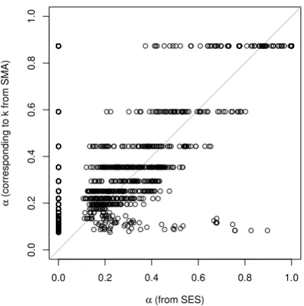
Lastly, we attempt to investigate the links between the selected optimal α values in the smoothing parameter of SES and the optimal orderk in SMA model. The latter have been converted to the former, using equation (2). Their relationship is graphically depicted in Figure 5. The horizontal axis presents the optimal values of α from the SES model, while the vertical axis presents the values of α that correspond to the optimal k orders of the SMA model. The grey diagonal line corresponds to the perfect correlation between the two variables. We observe that:
• The relationship proposed by Johnston et al. (1999) is not exact, especially if one focuses on the higher values of α.
0.0 0.2 0.4 0.6 0.8 1.0
0.0
0.2
0.4
0.6
0.8
1.0
α (from SES)
α
(
corresponding to
k from SMA
[image:15.595.189.407.107.326.2])
Figure 5: Relationship betweenαandkparameters for SES and SMA models.
• Just three values of k correspond to α values higher than 0.4 (vertical axis with α=
{0.87,0.59,0.44}). This finding, doubled with the superior performance of the SMA over the SES, suggests that extensive search within the parameter space of optimal values for the alpha smoothing parameter in the SES does not necessarily add value to forecasting performance in case of stationary data. In fact, a suboptimal selection of the smoothing parameter can result in similar (if not better) levels of accuracy. This result confirms the findings of a recent study by Nikolopoulos and Petropoulos (in press).
Overall, the SMA is a flexible model, that performs very well in terms of accuracy and bias. It is also easier to estimate and use than the SES. It is also important to note that the connection derived by Johnston et al. (1999) is only approximate and cannot be used as an exact connection between the SMA and the SES parameters.
5.2. Evaluation of prediction intervals
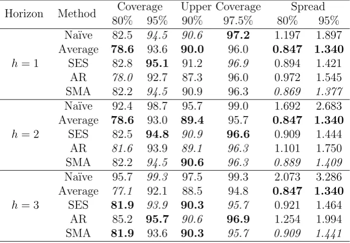
Table 5: Prediction intervals performance of the SMA against the Na¨ıve, the Average, the SES and the AR for different planning horizons.
Horizon Method Coverage Upper Coverage Spread
80% 95% 90% 97.5% 80% 95%
h= 1
Na¨ıve 82.5 94.5 90.6 97.2 1.197 1.897
Average 78.6 93.6 90.0 96.0 0.847 1.340
SES 82.8 95.1 91.2 96.9 0.894 1.421
AR 78.0 92.7 87.3 96.0 0.972 1.545
SMA 82.2 94.5 90.9 96.3 0.869 1.377
h= 2
Na¨ıve 92.4 98.7 95.7 99.0 1.692 2.683
Average 78.6 93.0 89.4 95.7 0.847 1.340
SES 82.5 94.8 90.9 96.6 0.909 1.444
AR 81.6 93.9 89.1 96.3 1.101 1.750
SMA 82.2 94.5 90.6 96.3 0.889 1.409
h= 3
Na¨ıve 95.7 99.3 97.5 99.3 2.073 3.286
Average 77.1 92.1 88.5 94.8 0.847 1.340
SES 81.9 93.9 90.3 95.7 0.921 1.464
AR 85.2 95.7 90.6 96.9 1.254 1.994
SMA 81.9 93.6 90.3 95.7 0.909 1.441
spread of the prediction intervals, the Average appear to be the best, following by the SMA model.
We can conclude that the superior performance of the SMA model in point forecast evaluation is coupled with a good prediction intervals performance that is close or even better to the levels of its main competitors (Average, SES and AR models). This observation is emphasised on the longer horizons. This means that on top of decreased working stock as a result of more accurate point forecasts, the SMA model results in a lower safety stock. However, in inventory control the more important element is the cumulative forecasts and respective prediction intervals, because the decision is usually based not on the average forecast of sales, but on the forecast of overall sales over the forecasting horizon.
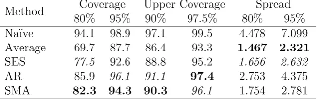
5.3. Evaluation of cumulative forecasts and prediction intervals
Table 6: Cumulative point forecast performance of the SMA against the Na¨ıve, the Average, the SES and the AR for the various error measures.
Method MAPE sMAPE MASE sME sMAE sMSE
Na¨ıve 31.578 28.126 2.578 0.079 0.816 1.931
Average 23.825 19.274 1.931 -0.020 0.573 0.902
SES 22.117 17.467 1.720 -0.013 0.531 1.008
AR 24.305 26.823 2.239 0.257 0.704 1.218
SMA 21.162 16.738 1.631 0.006 0.510 0.939
Table 7: Performance of the prediction intervals for the cumulative forecasts for the SMA against the Na¨ıve, the Average, the SES and the AR.
Method Coverage Upper Coverage Spread
80% 95% 90% 97.5% 80% 95%
Na¨ıve 94.1 98.9 97.1 99.5 4.478 7.099
Average 69.7 87.7 86.4 93.3 1.467 2.321
SES 77.5 92.6 88.8 95.2 1.656 2.632
AR 85.9 96.1 91.1 97.4 2.753 4.375
SMA 82.3 94.3 90.3 96.1 1.754 2.781
6. Conclusions
In this paper we have proposed simple statistical models underlying the simple moving average method. This proposition allows selecting automatically length of the SMA model, preserving observations and producing conditional mean and variance. This makes the SMA a more powerful instrument that can be used in practice for different purposes and gives statistical rationale for the method popular among practitioners.
We have conducted an experiment on real data and demonstrated the advantages of the proposed model over other existing simple level models, that are used in practice. We think that the good performance of the SMA in comparison with the SES and the Average on the stationary data that we used, can be explained by the ability of the SMA to take only several recent observations into account and distribute the weights between them uniformly. This means that the complete negligence of the old data is beneficial in terms of forecasting accuracy in this experiment.
The good performance of the SMA in terms of cumulative forecasts emphasises the point that this model can be efficiently used for inventory control systems. On one hand it outperforms all the other models used in the experiment in terms of point forecasts accuracy (which should lead to the reduction of working stock), while on the other hand it produces prediction intervals, covering the values very close to the nominal ones (suggesting that the targeted service levels are met).
[image:17.595.137.457.275.375.2]be preferred over SES or other level models. Particularly, we would suggest applying the SMA model to the other datasets featuring stationary series, ideally from different fields.
Appendix A. Cumulative Variance
In order to derive cumulative variance, the sum of actual values fromt+ 1 tot+h(where
h is the forecasting horizon) needs to be calculated:
Yt+h = h
X
j=1
y+j (A.1)
Here we assume that h > 1, because in case of h = 1 the cumulative variance is just equal to the variance of one-step-ahead forecast error. Inserting the measurement equations of (8) instead of actual values in (A.1) leads to:
Yt+h = h
X
j=1
(w0vt+j−1 +t+j) (A.2)
Any state vector value on the observationt+j (where j 6= 0) can be represented as:
vt+j =Fjvt+ j
X
i=1
Fj−igt+i, (A.3)
which can be inserted into (A.2) for all the j but j = 1 to obtain the following formula:
Yt+h = h
X
j=1
w0Fj−1vt+ h
X
j=2
j−1 X
i=1
w0Fj−i−1gt+i+t+j
!
+t+1. (A.4)
The second summation is done from j = 2 instead of j = 1, because the one-step-ahead actual value depends on vt and has only an error term t+1. So the cumulative sum of the actual values h-steps ahead is represented by (A.4) if we apply the state space model (8). The cumulative conditional mean of the model is then equal to:
µt+h|t= h
X
j=1
w0Fj−1vt, (A.5)
because the error term is assumed to have zero mean. The conditional variance is slightly more complicated and is calculated as:
σ2c,h = V (Yt+h|vt) = V h
X
j=2
j−1 X
i=1
w0Fj−i−1gt+i+t+j
!
+t+1 !
Regrouping elements in (A.6), the same variance can be written as:
σ2c,h = V t+h+ h−1 X
j=1 1 +
h−j
X
i=1
w0Fh−j−1g
!
t+j
!
. (A.7)
The partw0Fh−j−1g is repeated h−j times in (A.7), so the second sum can be substituted by theh−j:
σc,h2 = V t+h+
h−1 X
j=1
1 + (h−j)w0Fh−j−1gt+j
!
. (A.8)
Now taking into account the assumption of no autocorrelation in the residuals, the variance (A.8) can be rewritten as:
σc,h2 = V(t+h) + h−1 X
j=1
1 + (h−j)w0Fh−j−1g2V(t+j). (A.9)
Finally, if the assumption of homoscedasticity holds, then the variance of the error term will be constant leading to:
σ2c,h = 1 +
h−1 X
j=1
1 + (h−j)w0Fh−j−1g2
!
σ2. (A.10)
For simplicity the upper index h−j−1 in (A.10) can be substituted by j−1 without a loss in the derivations.
References
Ali, M. M., M. Z. Babai, J. E. Boylan, and A. A. Syntetos. 2015. “A forecasting strategy for supply chains
where information is not shared.”European Journal of Operational Research 260 (3): 984–994.
Ali, M. M., and J. E. Boylan. 2012. “On the effect of non-optimal forecasting methods on supply chain
downstream demand.”IMA Journal of Management Mathematics 23 (1): 81–98.
Davydenko, A., and R. Fildes. 2013. “Measuring Forecasting Accuracy: The Case Of Judgmental
Adjust-ments To Sku-Level Demand Forecasts.”International Journal of Forecasting 29 (3): 510–522.
Durbin, J., and S. J. Koopman. 2012. Time Series Analysis by State Space Methods. Oxford University
Press.
Franses, P. H., and R. Legerstee. 2009. “Properties of expert adjustments on model-based SKU-level
fore-casts.” International Journal of Forecasting 25: 35–47.
Franses, P. H., and R. Legerstee. 2011. “Combining SKU-level sales forecasts from models and experts.”
Expert Systems with Applications 38: 2365–2370.
Goodwin, P., and R. Lawton. 1999. “On the asymmetry of the symmetric MAPE.”International Journal
of Forecasting 15: 405–408.
Hyndman, R. J., and A. B. Koehler. 2006. “Another look at measures of forecast accuracy.”International
Journal of Forecasting 22 (4): 679–688.
Hyndman, R. J., A. B. Koehler, J. K. Ord, and R. D. Snyder. 2008.Forecasting with Exponential Smoothing.
Johnston, F. R., J. E. Boylan, M. Meadows, and E Shale. 1999. “Some Properties of a Simple Moving
Average when Applied to Forecasting a Time Series.” The Journal of the Operational Research Society
50 (12): 1267–1271.
Kolassa, S. 2016. “Evaluating predictive count data distributions in retail sales forecasting.”International
Journal of Forecasting 32 (3): 788–803.
Koning, A. J., P. H. Franses, M. Hibon, and H. O. Stekler. 2005. “The M3 competition: Statistical tests of
the results.”International Journal of Forecasting 21 (3): 397–409.
Makridakis, S., A. P. Andersen, R. Carbone, R. Fildes, M. Hibon, R. Lewandowski, J. Newton, E. Parzen, and R. L. Winkler. 1982. “The accuracy of extrapolation (time series) methods: Results of a forecasting
competition.” Journal of Forecasting 1 (2): 111–153.
Makridakis, S., and M. Hibon. 2000. “The M3-Competition: results, conclusions and implications.”
Inter-national Journal of Forecasting 16: 451–476.
Nikolopoulos, K., and F. Petropoulos. in press. “Forecasting for big data: does sub-optimality matter?.”
Computers & Operations Research .
Petropoulos, F., R. Fildes, and P. Goodwin. 2016. “Do ‘big losses’ in judgmental adjustments to statistical
forecasts affect experts’ behaviour?.”European Journal of Operational Research 249: 842–852.
Petropoulos, F., and N. Kourentzes. 2015. “Forecast combinations for intermittent demand.”Journal of the
Operational Research Society 66 (6): 914–924.
Rego, J. R. D., and M. A. D. Mesquita. 2015. “Demand forecasting and inventory control: A simulation
study on automotive spare parts.”International Journal of Production Economics 161: 1–16.
Sani, B., and B. G. Kingsman. 1997. “Selecting the Best Periodic Inventory Control and Demand Forecasting
Methods for Low Demand Items.”The Journal of the Operational Research Society 48 (7): 700.
Snyder, R. D. 1985. “Recursive Estimation of Dynamic Linear Models.” Journal of the Royal Statistical
Society, Series B (Methodological) 47 (2): 272–276.
Syntetos, A. A., and J. E. Boylan. 2006. “On the stock control performance of intermittent demand
esti-mators.”International Journal of Production Economics 103 (1): 36–47.
Tashman, L. J. 2000. “Out-of-sample tests of forecasting accuracy: an analysis and review.”International
Journal of Forecasting 16 (4): 437–450.
Wang, X., and F. Petropoulos. 2016. “To select or to combine? The inventory performance of model and
expert forecasts.” International Journal of Production Research 54 (17): 5271–5282.
Weller, M., and S. Crone. 2012. Supply Chain Forecasting: Best Practices and Benchmarking Study.
Tech-nical report. Lancaster Centre for Forecasting.
Winklhofer, H., A. Diamantopoulos, and S. F. Witt. 1996. “Forecasting practice: A review of the empirical