warwick.ac.uk/lib-publications
Manuscript version: Author’s Accepted Manuscript
The version presented in WRAP is the author’s accepted manuscript and may differ from the
published version or Version of Record.
Persistent WRAP URL:
http://wrap.warwick.ac.uk/102350
How to cite:
Please refer to published version for the most recent bibliographic citation information.
If a published version is known of, the repository item page linked to above, will contain
details on accessing it.
Copyright and reuse:
The Warwick Research Archive Portal (WRAP) makes this work by researchers of the
University of Warwick available open access under the following conditions.
Copyright © and all moral rights to the version of the paper presented here belong to the
individual author(s) and/or other copyright owners. To the extent reasonable and
practicable the material made available in WRAP has been checked for eligibility before
being made available.
Copies of full items can be used for personal research or study, educational, or not-for-profit
purposes without prior permission or charge. Provided that the authors, title and full
bibliographic details are credited, a hyperlink and/or URL is given for the original metadata
page and the content is not changed in any way.
Publisher’s statement:
Please refer to the repository item page, publisher’s statement section, for further
information.
VARIABLES
NICHOLAS M. ERCOLANI, SABINE JANSEN, DANIEL UELTSCHI
Abstract. We propose a novel complex-analytic method for sums of i.i.d. random variables that are heavy-tailed and integer-valued. The method com-bines singularity analysis, Lindel¨of integrals, and bivariate saddle points. As an application, we prove three theorems on precise large and moderate de-viations which provide a local variant of a result by S. V. Nagaev (1973). The theorems generalize five theorems by A. V. Nagaev (1968) on stretched exponential laws p(k) = cexp(−kα) and apply to logarithmic hazard func-tionscexp(−(logk)β),β >2; they cover the big jump domain as well as the small steps domain. The analytic proof is complemented by clear probabilistic heuristics. Critical sequences are determined with a non-convex variational problem.
1. Introduction
The motivation of the present article is two-fold. First, we present a new analytic method for the investigation of large powers of generating functions of sequences that satisfy some analyticity and log-convexity conditions. The method is explained and developed for probability generating functions but it has potentially broader applications and is motivated by techniques commonly used in analytic combina-torics [11]. Specifically, we show that methods akin to singularity analysis can be pushed beyond the realm of functions amenable to singularity analysis in the sense of [11, Chapter VI.1].
Second, we explore consequences for probabilistic limit laws and prove three the-orems on precise large and moderate deviations for sums of independent identically distributed (i.i.d.) random variables that are heavy-tailed [7] and integer-valued. The theorems generalize results on stretched exponential laws by A. V. Nagaev [15] which have recently attracted interest in the context of the zero-range process [2]. They are close in spirit to results by S. V. Nagaev [17], however with more concrete conditions on the domain of validity of the theorems, and provide deviations results “on the whole axis” [20]. Our assumptions are more restrictive than one may wish from a probabilistic perspective; in return, they allow for sharp results and may
Date: 21 April 2017.
1991Mathematics Subject Classification. 05A15; 30E20; 44A15; 60F05; 60F10.
Key words and phrases. local limit laws; large deviations; heavy-tailed random variables; as-ymptotic analysis; Lindel¨of integral; singularity analysis; bivariate steepest descent.
Department of Mathematics, The University of Arizona, Tucson, AZ 85721–0089, ([email protected]). Supported by NSF grant DMS-1212167.
Department of Mathematics, University of Sussex, Falmer Campus, Brighton BN1 9QH, United Kingdom ([email protected]).
Department of Mathematics, University of Warwick, Coventry, CV4 7AL, United Kingdom ([email protected]).
1
provide a helpful class of explicit reference examples. For example, we prove that one of the bounds of the (local) big-jump domain for logarithmic hazard functions derived in [4] is sharp.
The analytic proof of the theorems is complemented by clear probabilistic heuris-tics. Our results cover different regimes: a small steps or moderate deviations regime, where a classical variant of a local central limit theorem with corrections expressed with the Cram´er series holds [12], and a big-jump regime where the large deviation is realized by making one out of then variables large. In the language of statistical mechanics and the zero-range process, they correspond to supersatu-rated gas and a condensed phase [2]. The critical scales that distinguish between regimes are defined with the help of a non-convex variational problem which en-codes competing probabilistic effects. This complements the approach taken by Denisov, Dieker and Shneer [4].
The study of combinatorial generating functions shares much in common with the study of probability generating functions; in fact in many instances they coincide or run parallel as is the case for more recent investigations in the area of random combinatorial structures [1]. From the viewpoint of complex function theory the key here involves relating asymptotic questions to questions about the nature of the singularities of generating functions viewed as more global analytic objects. In most of the successful applications of thissingularity analysisto coefficient asymptotics a bridge is provided by the realization that the series in question satisfies some global algebraic or differential equation. Generating functions for which this is the case are referred to as holonomic. Pushing beyond this class in a systematic way requires new ideas and one of the most promising of these is the use of Lindel¨of integrals. Lindel¨of introduced these classically [13] as a means to constructively carry out analytic continuations of function elements (series) in a fairly general setting. In more recent times his construction has begun to be used to study non-holonomic combinatorial generating functions [10]. The generating functions for heavy-tailed distributions studied in this paper are of non-holonomic type and our methods of studying them show a new application of Lindel¨of’s construction that has novel connections to other areas of analytic asymptotic analysis such as bivariate steepest descent. In future work we hope to build on the present article in a way that broadens the application of harmonic analysis and complex function theory to problems of asymptotic analysis in both probability and combinatorics, such as applying the theory of Hardy spaces and Riemann-Hilbert analysis and extensions of Tauberian theorems as originally envisioned by Paley and Wiener [9]. Our proof shares some features with [17], where cumulative distribution func-tions are approximate Laplace transforms and approximating moment generating function admit analytic extensions (see Section 7). Contour integrals that appear in inversion formulas are deformed and analyzed by Gaussian approximation—our proof details in Section 5.4 follow [17]. There are, however, key differences: we need not deal with approximation errors because of stronger analyticity assump-tions, and our detailed analysis of the underlying variational problem allows us to formulate more concrete conditions for our theorems.
in the remaining sections. Steps 1 and 2 concern analytic extensions and notably use the Lindel¨of and Bromwich integrals (Section 4). Steps 4 and 5 analyze the critical points of a bivariate function and deal with the Gaussian approximation to a double integral (Section 5). The pivotal Step 3 connects the contour integral and the bivariate double integral; it leads to the full proof of our theorems that can be found in Section 6. In Section 7 we sketch how the method developed in this paper may be extended to more general settings, in particular when the analyticity required by our proof methods is not a priori given.
2. Results
We use the notationan∼bn :⇔an= (1 +o(1))bn andanbn:⇔an =o(bn).
2.1. Preliminaries. In order to formulate the results, we need to introduce crit-ical sequences deduced from a variational problem and the Cram´er series. Let X, X1, X2, . . .be independent, identically distributed random variables with values inNand law
P(X=k) =p(k) = exp(−q(k)) (k∈N) (2.1)
for some sequence (q(k))k∈N. We assume thatX is heavy-tailed and has moments of all orders, i.e., the generating function
G(z) =
∞ X
k=1
p(k)zk (|z| ≤1) (2.2)
has radius of convergence 1 and E[Xm] = P∞k=1k
mp(k)<∞for all m∈
N. Let
µ and σ2 be the expectation and variance of X. Set S
n = X1+· · ·+Xn. We
are interested in the asymptotic behavior ofP(Sn =µn+Nn) whenn, Nn → ∞
with Nn
√
n. The following assumption is similar to conditions considered by S. V. Nagaev [17].
Assumption 2.1. For some a > 0, the sequence (q(k))k∈N∩(a,∞) extends to a smooth functionq: (a,∞)→Rwhich has the following properties:
(i) q0 >0,q00<0, andq(3)>0. (ii) limx→∞xq0(x)/(logx) =∞.
(iii) c1
q0(x)
x ≤ |q
00(x)| ≤c
2
q0(x)
x for some constantsc1, c2>0.
(iv) c3|q00x(x)|≤q(3)(x)≤c4|q00(x)|
x for some constantsc3, c4>0.
(v) q0(x)≤αq(xx) for someα∈(0,1).
Assumption 2.1 allows for an easy analysis of an auxiliary variational problem, which is essential to the formulation of our main results. Let us collect a few elementary consequences. Under Assumption 2.1,q is concave on (a,∞) and p= exp(−q) is log-convex. Moreover, limx→∞x2q00(x)/logx=−∞and fory > x > a,
using
q0(y) q0(x) = exp
−
Z y
x
|q00(u)|
q0(u) du
, (2.3)
we estimate
y
x
−c2
≤ q
0(y)
q0(x) ≤ y
x
−c1
≤1 (2.4)
Similarly, fory > x > a,
y
x
c3
≤ q
00(y)
q00(x)≤ y
x
c4
SinceG(z) =P
kz
kexp(−q(k)) has radius of convergence 1, we also know that
lim
x→∞q
0(x) = lim
x→∞q
00(x) = lim
x→∞q
(3)(x) = 0. (2.6)
Indeed by Assumption 2.1,q0is eventually decreasing and the limit`:= limx∞q0(x)
exists inR∪ {−∞}. Then`= limx→∞q(x)/xandG(z) has radius of convergence
exp(`) = 1, whence`= 0. Assumption 2.1(iii) and (iv) leads to the statements on higher order derivatives. Assumption 2.1(v) impliesq(x) =O(xα) asx→ ∞.
Our method of proof requires two more analyticity assumptions, though in Sec-tion 7 we discuss how, following [17], one might be able to relax these assumpSec-tions.
Assumption 2.2. There existsb≥0 such that (p(n))n∈N∩[b,∞)extends to a func-tionp(ξ) that is continuous on a closed half-plane Reξ ≥b, analytic on the open half-plane Reξ > b, and in addition satisfies
(i) For everyε∈(0, π), some Cε>0, and allξ, we have|p(ξ)| ≤Cεexp(ε|ξ|).
(ii) R∞
−∞|(b+ is)
kp(b+ is)|ds <∞for allk∈
N.
Moreoverp(x) = exp(−q(x)) for allx≥max(a, b) witha,q(x) as in Assumption 2.1.
Assumption 2.3. Letp(ξ) = exp(−q(ξ)) be the analytic extension from Assump-tion 2.2, defined in Reξ≥b. Thenq(ξ) =−Logξ, defined with the principal branch of the logarithm is analytic as well, and the following holds:
(i) Forr >0 large, letzr=b+ i
√
r2−b2. Then asr→ ∞,
Z
Reξ=b,|ξ|≥r
exp(−Req(ξ))dξ
≤exp(−Req(zr) +O(logr)).
(ii) Im (ξq0(ξ))≤Im (ξq0(r)) for all largerand allξwith Imξ≥0 and|ξ|=r. (iii) |q(3)(ξ)| ≤C|q00(ξ)/ξ|for someC >0 and allξ.
Assumption 2.3 enters the proof of Theorem 4.4 only.
Variational problem and critical scale. Assumption 2.1 is tailored to the analysis of an auxiliary variational problem, motivated by the following heuristics. For subexponential random variables, the typical large deviations behavior is realized by making one out of thenvariables large,
P(Sn=µn+Nn)≈nP(Xn =Nn−kn)P(Sn−1=µn+kn) (2.7)
with a yet to be determined optimal kn. Assuming that a normal approximation
for the second factor is justified, we get
P(Sn=µn+Nn)≈exp
−q(Nn−kn)−
k2
n
2nσ2
(2.8)
where we have neglected prefactors n and 1/√2πnσ2 (see Eq. (2.11) below for a more refined heuristics). The optimal kn is then determined by minimizing the
term in the exponential. Thus we are led to the minimization of
fn(x) =q(x) +
(Nn−x)2
2nσ2 . (2.9)
As illustrated in Figure 1, the nature of the variational problem changes withNn.
Definex∗n>0 andNn∗ by
q00(x∗n) =− 1
nσ2, N
∗
n =x∗n+nσ
2q0(x∗
For sufficiently large n, the inflection pointx∗n is uniquely defined because of the
monotonicity from Assumption 2.1 and Eq. (2.6), moreoverx∗n → ∞. The quantity
Nn∗ is defined in such a way that the tangent to the curvey=q0(x) atx=x∗n has
equationy= (N∗
n−x)/(nσ2), see Fig. 3.
The next two lemmas characterize the minimization of fn; they are proven in
Section 5.1. The first lemma relates the critical points offn to the location of Nn
compared toNn∗.
Lemma 2.4. For sufficiently large n, the following holds true:
(a) IfNn< Nn∗, thenfn0 >0 on(a,∞).
(b) If Nn = Nn∗, then fn0 has the unique zero x∗n, moreover fn0(x) ≥ 0 with
equality if and only ifx=x∗
n.
(c) IfNn> Nn∗andlim supn→∞Nn/(nσ2)<limx&aq0(x), thenfn has exactly
two critical pointsxn andx0n, which satisfyx0n< x∗n < xn< Nn and
fn(x0n) = max
(a,x∗
n)
fn, fn(xn) = min
(x∗
n,∞) fn.
(d) IfNn> Nn∗andlim infn→∞Nn/(nσ2)>limx&aq0(x), thenfnhas a unique
critical pointxn. It satisfiesxn∈(x∗n, Nn)and is a global minimizer.
ForNn > Nn∗, the functionfn may have two local minimizers: aand xn, and we
may wonder which one is the global minimizer. The answer depends on the location of Nn compared to a new critical sequenceNn∗∗. Concrete examples are given in
Sections 2.3 and 2.4.
Lemma 2.5. Forn sufficiently large, there is a uniquely defined N∗∗
n > Nn∗ such
that:
(a) IfN∗
n< Nn< Nn∗∗, thenfn(a)< fn(xn).
(b) If Nn=Nn∗∗, then fn(a) =fn(xn).
(c) If Nn> Nn∗∗, then fn(xn)< fn(a).
In general it may not be straightforward to determineNn∗∗ exactly, but it is simple
to find a lower bound: if a = 0 andq(Nn) < Nn2/(2nσ2), then Nn > Nn∗∗. This
lower bound corresponds, roughly, to the sequence Λ(n) in [17]. The sequences introduced up to now are ordered as follows.
Lemma 2.6. As n→ ∞, we have
√
nx∗n< Nn∗< Nn∗∗=O(n1/(2−α))n,
and for some constants C, δ >0
(1 +δ)x∗n≤Nn∗≤Cx∗n.
The lemma is proven in Section 5.1. Lemmas 2.4 and 2.5, together with the heuris-tics described above, suggest that forNn > Nn∗∗ the unlikely eventSn=nµ+Nn
is realized by making one component of the order ofxn. One may wonder how far
xn is from swallowing all of the overshootNn.
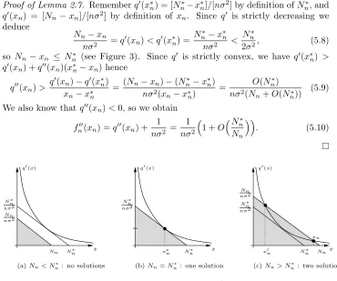
Lemma 2.7. Suppose Assumption 2.1(i) holds true. Let Nn> Nn∗. Then
Nn−Nn∗≤xn≤Nn, nσ2fn00(xn) = 1−nσ2|q00(xn)|= 1 +O
N∗
n
Nn
fn(x)
fn(x) fn(x)
x
x x
Nn2 2nσ2
Nn x0n x∗n xn Nn Nn
Nn2 2nσ2
Nn2 2nσ2
x0n x∗n xn q(Nn)
q(Nn)
(c)Nn> Nn∗∗ (b)N∗
n< Nn< Nn∗∗ (a)Nn< Nn∗
[image:7.612.168.480.380.496.2]q(Nn)
Figure 1. Minimization offn(x) =q(x) + (Nn−x)2/(2nσ2) and
illustration of Lemmas 2.4 and 2.5 for weightsq: (0,∞)→Rwith
q(0) = 0. For Nn > Nn∗, fn(x) has two critical points x0n and
xn separated by an inflection point x∗n. The global minimum is
reached either atx=xn or atx= 0.
In particular, forNn Nn∗, we have xn ∼Nn and nσ2f00(xn)→ 1. The lemma
is proven in Section 5.1. The information on the second derivative enters a refined heuristics: we make the ansatz that conditional on the unlikely eventSn=nµ+Nn,
there is one large component of sizexn, but the size is not deterministic. Instead,
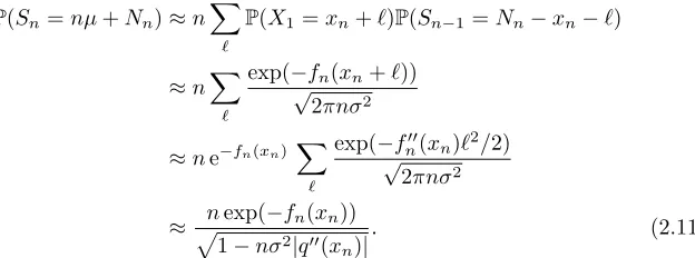
there are fluctuations aroundxn. This yields
P(Sn =nµ+Nn)≈n
X
`
P(X1=xn+`)P(Sn−1=Nn−xn−`)
≈nX
`
exp(−fn(xn+`))
√
2πnσ2
≈ne−fn(xn)X
`
exp(−fn00(xn)`2/2)
√
2πnσ2
≈pnexp(−fn(xn))
1−nσ2|q00(x
n)|
. (2.11)
Theorem 2.11 below confirms the heuristics for large Nn, up to correction terms
both in the prefactor and in the exponential.
Cumulants and Cram´er series. The heuristics together with Lemma 2.7 suggest that the optimal kn =Nn−xn in Eq. (2.8) is of order up toNn∗
√
n. At this scale the normal approximation fails and requires correction terms. The latter are usually expressed with the Cram´er series [12], whose definition we briefly recall. Letϕ(t) be the cumulant generating function ofX,
ϕ(t) = logE[ etX] = logG( et) (Ret≤0). (2.12)
Noteϕ(0) = 0. Ast→0,ϕ(t) can be approximated to arbitrary order
ϕ(t) =
r
X
j=1 κj
tj j!+O(t
r+1) (2.13)
with finite and real expansion coefficients κj ∈ R, the cumulants, see Section 4.
Definition 2.8. Let t(τ) = σ12τ+ P
j≥2ajτj be the formal power series obtained
by inverting
σ2t(τ) +X
j≥2 κj+1
t(τ)j
j! =τ.
The Cram´er series P
j≥0λjτj is the formal power series defined by composing the
expansion oft(τ)with the expansion of (µ+τ)t−ϕ(t),
(µ+τ)t(τ)−X
j≥1 κj
t(τ)j
j! =−
τ2 2σ2 +τ
3X
j≥0 λjτj.
Equivalently, the Cram´er series is the left-sided Taylor expansion of the Legendre transformϕ∗ at µ: letϕ∗(x) := supt≤0(tx−ϕ(t)). Then asτ%0,
ϕ∗(µ+τ) =− τ
2
2σ2 +τ 3
r
X
j=0
λjτj+O(τr+4) (2.14)
to arbitrarily high orderr.
Remark 1. Fort >0, log[P
k≥1p(k) exp(kt)] is infinite and the standard convention is to setϕ(t) =∞; thenϕ∗(µ+τ)≡0 forτ≥0 and Eq. (2.14) no longer applies. We adopt a different convention, however, for whichϕ(t) is smooth in a neighborhood of 0 (see Theorem 4.2), though it becomes complex-valued, and Eq. (2.14) applies to (Reϕ)∗ for positiveτ as well.
2.2. Main theorems. Setfn0=fn and forr≥1,
fnr(x) =q(x) +
(Nn−x)2
2nσ2 −
(Nn−x)3
n2
r−1
X
j=0 λj
Nn−x
n
j
. (2.15)
Remember the minimization of fn(x) and the critical scales
√
n Nn∗ < Nn∗∗ =
O(n1/(2−α))nillustrated in Fig. 1. In Proposition 2.12 below we check that the properties offn carry over tofnr. The following theorems provide a local variant
of a large deviations theorem by S. V. Nagaev [17], see also [18, Theorem 2.1]. The principal difference, apart from the local character of the theorems, is that our detailed investigation of the variational problem and notably Lemma 2.7 allows us to formulate conditions directly in terms of Nn, whereas S. V. Nagaev’s criteria
included an indirect condition on the sign of some second derivative.
Theorem 2.9. Let Nn→ ∞ with
√
nNn≤(1 +o(1))Nn∗. Pickrlarge enough
so that n(Nn/n)r→0. Then
P(Sn=µn+Nn)∼
1
√
2πσ2nexp
− N
2
n
2nσ2 + N3
n
n2
r−1
X j=0 λj Nn n j .
Theorem 2.10. LetNn → ∞withlim infNn/Nn∗>1andNn =O(n1/[2−α]). Pick
r large enough so thatn(Nn∗/n)r→0. Then
P(Sn=µn+Nn) = (1 +o(1))
1
√
2πσ2nexp
− N
2
n
2nσ2 + N3
n
n2
r−1
X j=0 λj Nn n j
+ (1 +o(1))p n 1−nσ2|q00(x
nr)|
exp−fnr(xnr)
withxnr=Nn+O(Nn∗) the largest solution offnr0 (xnr) = 0.
Lemma 2.5 suggests that for Nn Nn∗∗, the first contribution dominates and for
Nn Nn∗∗ the second contribution wins, but one has to be careful because of the
factorsnand 1/√2πnσ2as well as the Cram´er corrections; a detailed evaluation is best left to concrete examples (see, however, Corollary 2.13 below).
Theorem 2.11. Let Nn → ∞ with Nn n1/(2−α). Pick r large enough so that
n(Nn∗/n)r→0. Then
P(Sn =µn+Nn)∼nexp
−fnr(xnr)
withxnr=Nn+O(Nn∗) the largest solution offnr0 (xnr) = 0.
In practice one may prefer not to deal with the Cram´er corrections or the variational problem, and the following proposition is helpful.
Proposition 2.12. Suppose that lim infn→∞Nn/Nn∗ > 1. Fix r ∈ N0. Then,
for sufficiently large n,xnr is the maximizer of fnr restricted to (x∗n, Nn)and the
unique zero of fnr0 in that interval. Moreover 1−nσ2|q00(x
nr)| = 1 +O(Nn∗/Nn)
stays bounded away from zero and
xnr=Nn−(1 +o(1))nσ2q0(xnr) =Nn+O(Nn∗),
fnr(xnr) =q(xnr) +
1
2(1 +o(1))nσ 2q0(x
nr) =q(Nn)
1 +ON
∗
n
Nn
.
The proposition is proven in Section 5.1. For Nn Nn∗, we obtain xnr ∼ Nn,
q0(xnr)∼q0(Nn), andq(xnr) =q(Nn)−(1 +o(1))nσ2q0(Nn), hence
fnr(xnr) =q(Nn)−
1
2(1 +o(1))nσ 2q0(N
n)2. (2.16)
Now suppose in addition that lim inf Nn2
2nσ2/q(Nn)>1. Then in Theorem 2.10, the
first summand is of order exp(−(1 +o(1))N2
n/(2nσ2), the second of order exp(−(1 +
o(1))q(Nn)), so the first contribution is negligible and the validity of Theorem 2.11
extends accordingly, since 1−nσ2|q00(x
nr)| → 1 for Nn Nn∗. Eq. (2.16) now
yields the following corollary.
Corollary 2.13. TakeNn→ ∞withNn Nn∗ andlim inf Nn2
2nσ2/q(Nn)>1. Then
P(Sn=nµ+Nn)∼ne−q(Nn) =nP(X=Nn)
if and only if √nσ2q0(N
n)→0.
In concrete examples, Theorem 2.9 should allow us to extend the domain of validity of the corollary toNn Nn∗∗. The condition
√
nσ2q0(N
n)→0 is closely related to
theinsensitivity scale discussed by Denisov, Dieker and Shneer [4], as
p(Nn±
√
nσ2
p(Nn)
→1 ⇔√nσ2q0(N
n)→0. (2.17)
Remark 2 (Big-jump vs small steps). The domain where P(Sn = nµ+Nn) ∼
nP(X =Nn) is sometimes calledbig-jump domain. Think ofSn as the position of a
random walker with step size distributionp(k). In the situation of Corollary 2.13, the unlikely event that the walker has travelled a distance µn+Nn much larger
than the expected distanceµnis realized by one big jump of sizeNn. Finding the
The interpretation of Theorem 2.9, in contrast, is that the moderate overshoot Nn is achieved by a collective effort: all steps tend to stay small, though each
stretches a little beyond its expected valueµ. For stretched exponential variables, this interpretation is made rigorous in [15] and [2].
Remark 3 (Condensation in the zero-range process). In the zero-range process, the random variables X1, . . . , Xn model the number of particles at lattice sites
j = 1, . . . , n, with Sn the total number of particles, and µ is a critical density.
Theorem 2.9 corresponds to supersaturated gas. In Corollary 2.13, the particle excess Nn is absorbed by a condensate, i.e., one large occupation number. In
Theorem 2.11, the particle excess is shared by a condensate of sizexnr < Nn and
supersatured gas. See [2] and [8, Section 7].
We conclude with an equivalent but more intrinsic formulation of Theorem 2.11. In Section 4 we shall see that G(z) extends to a function that is analytic in the slit plane C\[1,∞), and in addition the limit G( et) = limε&0G( et + iε) exists for all t ≥0. So the cumulant generating functionϕ(t) = logG( et) extends to a function that is well-defined and smooth in a neighborhood of the origin inR, and
Eq. (2.13) stays valid for small positivet. We define
Φn(t, ξ) =−q(ξ) +nReϕ(t)−(µn+Nn)t+tξ
=−q(ξ) +n
r−1
X
j=2 κj
tj
j!−t Nn−ξ) +O(t
r). (2.18)
The asymptotic expansion holds for every order r. For Nn Nn∗ and sufficiently
largen, the bivariate function Φn(t, ξ) has exactly two critical points in (0,nσNn2)×
(a,∞). We label them as (tn, ξn) and (t0n, ξn0) withtn< t0n. Then, in the situation
of Theorem 2.11, we have
P(Sn =nµ+Nn)∼neΦn(tn,ξn). (2.19)
It is in this form that we prove the theorem. Let us explain how to recover the expression in terms offnr. We may solve for∇Φn(t, ξ) = 0 in two steps: (1) use
∂tΦn(t, ξ) = 0 to express t =t(ξ) as a function ofξ, (2) plug the expression into
∂ξΦn(t, ξ) to obtain an equation for ξ. This latter step breaks into the following
two stages:
(2a) substitute the expression oft =t(ξ) into the expression for Φn(t, ξ) so as
to obtain a function Φn(t(ξ), ξ) ofξ only;
(2b) set the derivative of Φn(t(ξ), ξ) with respect to ξto zero,
which is valid since d
dξΦn(t(ξ), ξ) = ∂Φn
∂ξ (t(ξ), ξ) + ∂Φn
∂t (t(ξ), ξ) dt dξ(t) =
∂Φn
∂ξ (t(ξ), ξ). (2.20)
By the definition of the Cram´er series, step (2a) gives
Φn(t(ξ), ξ) =−q(ξ)−
(Nn−ξ)2
2nσ2 +
(Nn−ξ)3
n2
X
j≥0 λj
Nn−ξ
n
j
(2.21)
Truncation of the asymptotic expansion on the right-hand side gives precisely the function−fnr(ξ). Forrlarge enough, step (2b) shows that we may approximate
Φn(tn, ξn) =−fnr(xnr) +o(1), nσ2q00(ξn) =nσ2q00(xnr) +o(1) (2.22)
2.3. Application to stretched exponential laws. Here we explain how to re-cover five theorems by A. V. Nagaev [15] for stretched exponential variables. Let α∈(0,1),c >0, and
p(k) =cexp(−kα), q(k) =kα−logc (k∈N). (2.23)
We need not check Assumption 2.3 since Theorem 4.4 for stretched exponential weights has already been proven in [12, Theorem 2.4.6].
Lemma 2.14. The probability weights (2.23)satisfy Assumptions 2.1 and 2.2, and we have
x∗n=
α(1−α)nσ21/(2−α), Nn∗=
2−α 1−αx
∗
n, Nn∗∗=Cα(nσ2)1/(2−α)
with Cα = (2−α)(2−2α)−(1−α)/(2−α). Moreover
√
nσ2q0(N
n)→0 if and only if
Nnn−1/(2−2α).
The proof of the lemma is sketched in Appendix A. The critical scalen−1/(2−α) is explained by a simple scaling relation: forNn =kn1/(2−α), we have
fn yn1/(2−α)
=nα/(2−α)yα+(k−y) 2
2σ2
−logc. (2.24) A careful examination of the expressions in Theorem 2.10 shows that the first summand dominates if Nn ≤ (1−δ)Nn∗∗ while the second dominates if Nn ≥
(1 +δ)Nn∗∗for someδ >0. In particular, Theorem 2.9 extends toNn≤(1−δ)Nn∗∗,
which corresponds to Theorem 1 in [15]. Theorem 2.10 forNn ∼Nn∗∗is Theorem 4
in [15]. ForNn ≥(1 +δ)Nn∗∗, we have
P(Sn =nµ+Nn)∼
1
p
1−nσ2q00(x
nr)
e−fnr(xnr). (2.25)
This regime can be divided into three cases:
(a) Nnn−1/(2−2α)corresponds to Theorem 2 in [15].
(b) WhenNn is of the order ofn−1/(2−2α), the corrections from the Cram´er series
are irrelevant and
P(Sn=µn+Nn)∼nexp −fn(xn), (2.26)
i.e., we may chooser= 0. This corresponds to Theorem 6 from the erratum [16], replacing Theorem 5 in the original article [15]. The statement actually extends to Nn n−1/(3−3α). Indeed q0(xnr) ∼ (Nn−xnr)/(nσ2) = o(Nn/n) yields
Nn−xnr= (1 +o(1))nσ2αNnα−1 and
fnr(xnr) =fn(xnr) +O nNn−(3−3α)
, (2.27)
and one can check thatfn(xnr) =fn(xn) +o(1) ifNnn−1/(3−3α).
(c) Nnn−1/(2−2α)corresponds to Theorem 3 in [15] and our Corollary 2.13.
2.4. Application to logarithmic hazard functions. Here we specialize to
p(k) =cexp −(logk)β
, q(k) =−logc+ (logk)β (2.28)
withβ >2.1
Lemma 2.15. The weights (2.28)satisfy Assumptions 2.1– 2.3. Moreover
Nn∗∼2x∗n∼2
q
21−ββnσ2(logn)β−1, N∗∗
n ∼
q
2nσ2(logn)β,
and√nσ2q0(N
n)→0if and only if Nn
√
n(logn)β−1.
The lemma is proven Appendix A. Notice that unlike the stretched exponential case (Lemma 2.14),Nn∗∗ is much larger thanNn∗. The scaling relation (2.24) is modified as follows: forNn=k
p
nσ2(logn)β−1∼kx∗
n, we have
fn(yx∗n) = (logx∗n)
β+β(logn)β−1logy+(k−y)2 2
+o(logn)β−1 (2.29)
and (logx∗
n)β∼(logn)β∼(logNn)β.
Our results may now be applied to obtain a sharp boundary for the big-jump domain.
Theorem 2.16. Let p(k) be as in Eq. (2.28) with β > 2 and Nn
√
n. Then
P(Sn=µn+Nn)∼nP(X =Nn)if and only ifNn
√
n(logn)β−1.
The “if” part of the theorem is actually a special case of [4, Theorem 8.2] and as such not new. The “only if” part shows that the boundary derived in [4] is in fact sharp.
Proof Theorem 2.16. Let In :=
√
nσ2(logn)β−1 and notice I
n Nn∗∗ for β >2.
Suppose that Nn In. Then we have, in particular, Nn Nn∗∗. Write Nn =
αnNn∗∗ withαn→ ∞. Then
N2
n/(2nσ2)
(logNn)β
=α2n1 +o(1)logαn logn
−β
≥ α
2
n
(logαn)β
→ ∞ (2.30)
and it follows from Corollary 2.13 that P(Sn = nµ+Nn) ∼ nP(X = n), hence
Nn Nn∗∗ is indeed a sufficient condition. In order to check that it is necessary,
we treat the caseNn=O(In) with Theorems 2.9 and 2.10.
Case 1: Nn∗ Nn = O(In). In Theorem 2.10 we obtain a lower bound by
neglecting the first contribution and estimating 1−nσ2|q00(x
nr)| ≤1. Combining
with Proposition 2.12, we find
P(Sn=nµ+Nn)≥nexp(−fnr(xnr) +o(1))
≥nexp−q(Nn) + (1 +o(1))nσ2q0(Nn)2+o(1)
(2.31)
hence in view ofNn =O(In) and Lemma 2.15
lim inf
n→∞
P(Sn=nµ+Nn)
nP(X =Nn)
≥lim inf
n→∞ exp (1 +o(1)nσ
2q0(N
n)2)
>1. (2.32)
Case 2: Nn =O(Nn∗). Then we have in particularNn =o(Nn∗∗). WriteNn =
αnNn∗∗ withαn→0, then
N2
n
2nσ2(logN
n)β
≤α
2
n(logn)β
(log√n)β →0 (2.33)
and Theorems 2.9 and 2.10 show
logP(Sn=nµ+Nn) nP(X =Nn)
≥ − N
2
n
2nσ2 + (logNn)
β+O(logn)→ ∞. (2.34)
3. Proof strategy
Here we explain the strategy for the proof of Theorems 2.9–2.11. We focus on the case Nn = o(n) and Theorem 2.10. Set m = µn+Nn. We start from the
observation that P(Sn = m) is equal to [zm]G(z)m, the coefficient of zm in the
expansion ofG(z)m, which in turn is given by contour integrals
[zm]G(z)n = 1 2πi
I G(z)n
zm
dz
z =
1 2πi
Z 2πi
0
enϕ(t)−mtdt. (3.1)
The contour integral can be taken over any circle centered at the origin with radius r ≤ 1. A steepest descent ansatz would look for a point zn such that
znG0(zn) =m/n=µ+Nn/n, or ηn withϕ0(ηn) = µ+Nn/n, and then integrate
over |z| =|zn| (or Ret = Reηn). However in the regime m/n > G0(1) = µ that
we investigate there is no such point, and instead we follow an approach that is in the spirit of singularity analysis [11] but with several novel ingredients. Crucially, the generating functionG(z)does not fall into the class of functions which Flajolet and Sedgwick call “amenable to singularity analysis” [11][Chapter VI].
Step 1: Analytic extension to slit plane. Observe thatG(z) has an analytic extension to the slit plane C\[1,∞). This is proven with the help of the Lindel¨of
integral [13, 10], see Proposition 4.1. The key ingredient here is that p(ξ) is ana-lytic in a complex half-plane containing the integersk∈Nand growth slower than
exp((π−ε)|ξ|) asξ→ ∞.
Step 2: Behavior near the dominant singularity and along the slit.
The Lindel¨of integral actually shows that the analytic extension G(z) has well-defined limits asz approaches the slit [1,∞) from above or below, i.e., the limits limε&0G( et+ iε) and limε&0G( et−iε) exist for allt∈R. Moreover the imaginary
part along the slit is given by a Bromwich integral,
lim
ε&0ImG( e
t + iε) = 1
2i
Z 1/2+i∞
1/2−i∞
etξp(ξ)dξ (t≥0). (3.2)
The line of integration Reξ= 1/2 can be replaced by any other line Reξ=x >0.
Ast&0, the imaginary part vanishes faster than any power oft, whereas the real
part can be approximated to arbitrarily high order by a Taylor polynomial.
Step 3: Contour integrals. We may now deform the contour of integration: in thez-plane, we replace the circle of radius 1 by a Hankel-type contour consisting of a circle of radius eε and a piece hugging the segment [1, ε), see Figure 2. In the
t-plane, we replace the vertical segment joining 0 and 2πi by the three other sides of the rectangle with corners 0,ε,ε+ 2πi, 2πi. This yields
[zm]G(z)n= 1 2πi
Z ε
0
enϕ(t)−mtdt+
Z 2π
0
enϕ(ε+iθ)−m(ε+iθ)idθ
−
Z ε
0
enϕ(t+2πi)−m(t+2πi)dt. (3.3)
We focus onNn=o(n) and chooseε=ηn as the solution of
Reϕ0(ηn) =
m
n =µ+
Nn
(b) (a)
|z|= eε
|z|= 1
ε
[image:14.612.178.435.118.246.2]0 2πi
Figure 2. Contour integrals in thez-plane (a) and in thet-plane (b). Dotted lines: Eq. (3.1). Solid lines: deformed contours in Eq. (3.3). Recall that z = et. Later ε= ηn will be chosen in a
judicious way. ForNn Nn∗∗, the dominant contribution should
come from the horizontal pieces of the deformed contour in the t-plane. ForNnNn∗∗, the dominant contribution should instead
be from the vertical line.
Noticeηn ∼Nn/(nσ2). Using the identities
G(z) =G(z), ∀t≥0 : ϕ(t+ 2πi) =ϕ(t), (3.5)
Eq. (3.3) becomes
[zm]G(z)n =Hn+Vn (3.6)
with
Hn=
1 π
Z ηn 0
enReϕ(t)−mt sin nImϕ(t)
dt
Vn=
1 π
Z π
0
enReϕ(ηn+iθ)−mηn cos nImϕ(η
n+ iθ)dθ.
(3.7)
Standard arguments show that the dominant contribution toVn come from small
θ. Since ImG( et)→0 faster than any power of tast&0 and
ImG( et) = Im eϕ(t) = eReϕ(t)Imϕ(t)∼Imϕ(t), (3.8) we may drop the trigonometric functions from Eq. (3.7) and find
Hn∼
n π
Z ηn 0
enReϕ(t)−mtImG( et)dt,
Vn∼
1 π
Z π
0
enReϕ(ηn+iθ)−mηndθ.
(3.9)
The vertical contribution is evaluated with the help of a Gaussian approximation aroundθ= 0, which yields
Vn∼
1
p
2πnReϕ00(η
n)
With Definition 2.8, we recognize in Eq. (3.10) the asymptotic expression from Theorem 2.9 and obtain
Vn ∼
1
√
2πnσ2exp
− N
2
n
2nσ2 + N3
n
n2
r−1
X
j=0 λj
Nn
n
j
. (3.11)
The evaluation ofHnis more involved. As a preliminary step, we express ImG( et)
through the Bromwich integral and find
Hn∼
n 2πi
Z ηn 0
Z 1/2+i∞
1/2−i∞
eΦn(t,ξ)dξ
dt (3.12)
with Φn as in Eq. (2.18).
Step 4: Critical points of Φn(t, ξ). In order to apply a Gaussian
approxima-tion to the bivariate integral (3.12), we look for a critical points (tn, ξn) of Φn with
tn ∈(0, ηn) andξn∈(0,∞). The gradient∇Φn(tn, ξn) vanishes if and only if
tn=q0(ξn),
Re ϕ0(tn)−ϕ0(0)
= Nn−ξn
n .
(3.13)
Since Reϕ0(t) =µ+σ2t+O(t2) ast&0, Eq. (3.13) implies q0(ξn)∼
Nn−ξn
nσ2 . (3.14)
We recognize the equation for the critical points of fn. Lemma 2.4 suggests the
following: for Nn Nn∗, there should be no critical point, for Nn∗ Nn n,
there should be two. Let us focus on the latter case and label the critical points as (tn, ξn) and (t0n, ξ0n) with tn < t0n. In view of Lemmas 2.4 and 2.7, we expect
ξn≈xn andξn0 ≈x0n, hence
tn∼q0(Nn), ξn=Nn+O(Nn∗) (3.15)
andξ0n< x∗n< ξn. The Hessian of Φn is
Hess Φn(t, ξ) =
nReϕ00(t) 1 1 −q00(ξ)
. (3.16)
Using again Lemma 2.7 andξn≈xn, we expect
det Hess Φn(tn, ξn) =−1− 1 +o(1)
nσ2q00(ξn) =−1 +O
Nn∗
Nn
<0 (3.17)
thus (tn, ξn) is a saddle point. (More precisely, it is a saddle point of Re Φn, but
the abuse of terminology is natural and not problematic in our context.) On the other handξ0
n≈x0n < x∗n with 1 +nσ2q0(x∗n) = 0 by definition of x∗n, so we expect
det Hess Φn(t0n, ξn0) =−1− 1 +o(1)
nσ2q00(ξn0)>0. (3.18)
Step 5: Gaussian approximation for Hn. In order to evaluate the double
integral in Eq. (3.12), we use a good change of variables and a Gaussian approx-imation. Let ξ(t) be the solution of q0(ξ) =t, so that∂ξΦn(t, ξ) = 0 if and only
ifξ=ξ(t). It is convenient to deform the contour and integrate along Reξ=ξ(t) instead of Reξ= 1/2. The integral becomes
Hn∼
n 2π
Z ηn 0
Z ∞
−∞
A straightforward computation shows thatFn(t, s) =Sn(t, ξ(t) + is), a function of
two real variablest, s, has a critical point at (tn,0) with positive definite Hessian
HessFn(tn,0) =
βn 0
0 −∂ξ2Φn(tn, ξn)
, βn =
det Hess Φn(tn, ξn)
∂2
ξΦn(tn, ξn)
, (3.20)
see Lemma B.1. Fn : (0, ηn)×R→ C has another critical point at (t0n,0), with
negative determinant of the Hessian; later we show that it does not contribute to the integral. The evaluation ofHn is concluded by replacing the double integral (3.19)
by the integral of the Gaussian approximation around (tn,0) which yields
Hn∼
n 2π
s
(2π)2 det HessFn(tn,0)
eFn(tn,0) = n
p
|det Hess Φn(tn, ξn)|
eΦn(tn,ξn).
(3.21) The argument leading leading to Eq. (2.22) and Eq. (3.17) show
Hn∼
n
p
1−nσ2q00(x
nr)
e−fnr(xnr). (3.22)
4. Analytic continuation. Lindel¨of and Bromwich integrals
Here we take care of steps 1 and 2, starting from Assumption 2.2. For concrete-ness’ sake we write down the results for b = 1/2; they apply for general b with straight-forward modifications. Define
Λ(w) =− 1
2πi
Z 1/2+i∞
1/2−i∞
p(ξ)wξ π
sinπξdξ (w∈C\(−∞,0]), (4.1) the Lindel¨of integral with symbolp(ξ).
Proposition 4.1 ([13]).
(a) Λ(w)is analytic in the slit plane C\(−∞,−1].
(b) In the unit disk |w| ≤1,
Λ(w) =
∞ X
k=1
p(k)(−w)k=G(−w).
A detailed proof and many additional properties of Λ(w) can be found in [10]. Proposition 4.1 shows right away thatG(z) = Λ(−z) has an analytic continuation from the unit disk to the open slit planeC\[1,∞). We use the same letterG(z) for the analytic continuation, and setϕ(t) = LogG( et) with Log the principal branch
of the logarithm, and Imt∈[0,2π). We prove the following additional properties ofG(z) andϕ(t).
Theorem 4.2.
(a) The boundary valueG( et) = lim
ε&0G( et + iε)exists for all t∈Rand is
a smooth function oft∈R.
(b) The imaginary partImG( et),t≥0is given by the Bromwich integral(3.2).
(c) ϕ(t)is well-defined and smooth in a neighbourhood of the origin; the deriva-tives κj =ϕ(j)(0)are real. As t→0in the strip Imt∈[0,2π), we have
ϕ(t) = LogG( et) =
r
X
j=1 κj
tj
j! +O(t
r+1).
In (c)z = et is allowed to approach the slit [1,∞) as fast as we like; we may even take t real. Because the coefficients κj are real, we find in particular that
ImG( et) vanishes faster than any power oft ast→0,t∈R.
Proof of Theorem 4.2. Foru∈Cin the closed strip Imu∈[−π, π], define
L(u) =− 1
2πi
Z 1/2+i∞
1/2−i∞
p(ξ) eξu π
sinπξdξ. (4.2)
When Imuis in the open strip Imu∈(−π, π), we havew= eu ∈C\(−∞,0] and
L(u) = Λ( eu). Along the vertical line Reξ= 1/2, we have
exp(ξu) sin(πξ)
= 2 e
Reu/2 exp(−sImu)
exp(πs) + exp(−πs) ≤2 e Reu/2
(ξ=1
2 + is) (4.3)
By Assumption 2.2(ii), since ξkp(ξ) is integrable along Reξ = 1/2. Eq. (4.3)
then shows that the integral defining L(u) is absolutely convergent, and it stays absolutely convergent if we replace the symbolp(ξ) byξkp(ξ). Standard arguments
for parameter-dependent integrals then show thatL(u) is continuous on the closed strip, differentiable in the open strip, and we may exchange differentiation, limits, and integration, which shows that the restriction ofLto the boundaries Imu=±π yield smooth functions.
Whenz→ et ∈[1,∞) along Imz >0, we havew=−z→ −et along Imw <0. Thus we may writew= eu with Reu→tand Imu= argw& −π. Therefore
lim
ε&0G( e
t + iε) =L(t−iπ) = i
Z ∞
−∞
p 12+ is
e(1/2+is)t exp(πs)
exp(πs) + exp(−πs)ds. (4.4) This proves the existence of the limit and, in view of the above mentioned properties ofL(u), the smoothness as a function oft. The complex conjugate is
−i
Z ∞
−∞
p 12−is
e(1/2−is)t exp(πs)
exp(πs) + exp(−πs)ds = i
Z ∞
−∞
p 12+ is
e(1/2+is)t exp(−πs)
exp(πs) + exp(−πs)ds. (4.5) Therefore
ImG( et) =1 2
Z ∞
−∞
p 12+ is
e(1/2+is)tds= 1 2i
Z 1/2+i∞
1/2−i∞
p(ξ) etξdξ.
This proves (b). For (c), consider first real t ∈ R. We have already checked (a)
henceG( et) is inC∞(
R). It is real and strictly positive fort≤0 (this follows from
the series representation and p(k) > 0), and non-zero though possibly complex-valued for sufficiently small t >0. Therefore ϕ(t) = logG( et) is well-defined and
smooth in some interval (−∞, δ),δ > 0, and real-valued fort≤0. In particular, the derivatives κj =ϕ(j)(0) exist and are real, and ϕ(t) can be approximated to
arbitrarily high order by Taylor polynomials. The extension to complex t, Imt ∈
[0,2π), follows again from the smoothness ofL(u) in the closed strip Imu∈[−π, π].
Theorem 4.2(b) has an interesting consequence. Eq. (3.2) is, up to a factor π, the formula for the inverse Laplace transform, therefore
p(λ) =π
Z ∞
0
e−tλImG( et)dt (Reλ >0). (4.6)
In the special case of stretched exponential weights, we can draw on an extensive literature as exp(−λα) is known to be the Laplace transform of a probability density,
anα-stable law. Forα= 1/2 [5]
ImG( et) = c
√
π 2t3/2e
−1/(4t) (t≥0). (4.7)
For generalα∈(0,1), we have instead [12, Theorem 2.4.6]
ImG( et)∼ c
2
s
2π (1−α)α−1/(1−α)
exp −(1−α) α t
α/(1−α)
t(2−α)/(2−2α) (4.8)
as t & 0. This is proven in [12] by applying a steepest descent approach to the
Bromwich integral. For general weights, Eq. (4.8) is generalized as follows. Assume that t < limx&a|q00(x)|. By Assumption 2.1, q00 is strictly increasing
and negative on (a,∞). By Eq. (2.6), we haveq00(x)→0 asx→ ∞. Consequently there exists a uniquely definedξ(t) that solvesq0(ξ(t)) =t. We define
ψ(t) =tξ(t)−q(ξ(t)) (4.9)
and note the relations
ψ0(t) =ξ(t), ψ00(t) = 1
q00(ξ(t)), (4.10)
soψ(t) is monotone increasing and strictly concave. Since−ψ(−t) is the Legendre transform of the convex function−q(x), it comes as no surprise that Assumption 2.1 on largextranslates into information on smallt.
Lemma 4.3. The following holds:
(a) limt&0tψ0(t)/logt=∞.
(b) −ψ00(t)≥cψ0t(t) for somec >0 and all sufficiently small t >0. (c) 0≤ψ(3)(t)≤C|ψ00(t)|
t for someC >0and all sufficiently small t >0.
The lemma has been proven in [17, Lemma 2.2].
Theorem 4.4. As t&0,
ImG( et)∼ 1
2
p
2π|ψ00(t)| eψ(t).
Proof. By Theorem 4.2(b) we may start from the Bromwich representation of ImG( et). The analyticity of q(ξ) allows us to replace the contour Reξ = 1/2
by Γ = Γ1∪Γ2 where
Γ1={ξ∈C| |ξ|=ξ(t),Reξ≥1/2}, Γ2={ξ∈C| |ξ|> ξ(t),Reξ= 1/2}.
θwe have
t reiθ −q(reiθ) =ψ(t)−1
2r
2q00(r)( eiθ −1)2+O r3q(3)(r)( eiθ −1)2
=ψ(t)−1
2r
2|q00(r)| θ2+O(θ3)) (4.12) The estimate is uniform in r = ξ(t) by Assumption 2.3(iii). Let ε(r) & 0 with ε(r)2r2q00(r)/logr→ ∞(this is possible by Assumption 2.1), then
1 2i
Z ε(r) −ε(r)
exp treiθ −q(reiθ)
ireiθdθ∼ 1
2
p
2π|ψ00(t)|eψ(t). (4.13) As we veer away fromr=ξ(t) along Γ1, the real part ofξt−q(ξ) decreases. Indeed forθ∈(0, π/2)
d
dθRe tre
iθ −q(reiθ)
= Re iξ(t−q0(ξ)) ξ=reiθ =−Im ξq0(r)−ξq0(ξ)
ξ=reiθ ≤0. (4.14) At the very end we have used Assumption 2.3(ii) It follows that
1 2i
Z θ0
ε(r)
exp treiθ −q(reiθ)
ireiθdθ
≤rπ
4 exp
ψ(t)−1
2r
2|q00(r)|ε(r)(1 +o(1))=oexp(ψ(t))
Taking complex conjugates, we obtain a similar estimate for the integral from−θ0 to−ε(r). Together with (4.13) we obtain
1 2i
Z
Γ1
etξ−q(ξ)dξ∼ 1
2
p
2π|ψ00(t)|eψ(t). (4.15) It remains to estimate the contribution from Γ2. Because of the monotonicity (4.14) we have
Re (tξ0−q(ξ0))≤ψ(t)− 1 2r
2|q00(r)|ε(r)2(1 +o(1)) (4.16) Assumption 2.3(ii) ensures that
Z
Γ2
etξ−q(ξ)dξ ≤exp
Re
tξ0−q(ξ0)
+O(logr))=oexp(ψ(t)). (4.17)
5. Critical point and Gaussian approximation
Here we prove Lemmas 2.4-2.7 and Proposition 2.12 and we address steps 4 and 5 of the proof strategy.
5.1. Variational analysis offn(x). Critical scales.
Proof of Lemma 2.4. We treat the case a = 0. Under Assumption 2.1(i), q0 is strictly convex and decreasing. Therefore
fn0(x) =q0(x)−
Nn−x
nσ2
≥q0(x∗n) +q00(xn∗)(x−x∗n)−Nn−x
nσ2 =
Nn∗−Nn
nσ2
with equality if and only if x=x∗n. If Nn < Nn∗, we obtain fn0(x) >0 on (0,∞)
and parts (a) and (b) of the lemma follow right away.
IfNn > Nn∗, thenfn0(x∗n) = (Nn∗−Nn)/(nσ2)<0 and limx→∞fn0(x) =∞, so by
the intermediate value theoremf0
n has at least one zero in (x∗n,∞). On the other
hand
fn00(x) =q00(x) + (nσ2)−1=q00(x)−q00(x∗n)>0 on (x∗n,∞) (5.2) so fn0 is strictly increasing and fn0 has exactly one zero xn in (x∗n,∞), moreover
fn(xn) = min(x∗
n,∞)fn. Since q
0(x
n)>0 by Assumption 2.1 andq0(xn) = (Nn−
xn)/(nσ2), we must havexn < Nn. This proves the first part of (c).
If in addition toNn> Nn∗, we have lim supn→∞Nn/(nσ2)<limx&aq0(x), then
limx&afn0(x)>0. We have already observed thatfn0(x∗n)<0. By the intermediate
value theorem,fn0 has at least one zerox0nin (0, x∗n). Sincefn00(x) =q00(x)−q00(x∗n)< 0 on (0, x∗n), the zero is unique and corresponds to maximizer. This completes the proof of (c). The proof of (d) is similar to (c) and therefore omitted.
Proof of Lemma 2.5. We treat the case a = 0. Write fn(x) = In(x, Nn) with
In(x, y) = q(x) + [y−x]2/[2nσ2]. For y > Nn∗, let xn(y) > x∗n > x0n(y) be the
solutions of∂xIn(x, y) = 0, with x0n(y) well-defined for Nn ≤nσ2supq0 only.
No-tice thatx7→In(x, y) is increasing in (0, x0n(y)), decreasing in (x0n(y), xn(y)), and
increasing in (xn(y),∞). We have
d dy
In(xn(y), y)−I(0, y)
=y−xn(y)
nσ2 −
y nσ2 =−
xn(y)
nσ2 <0. (5.3)
As y & Nn∗ at fixed n, a careful examination of the proof of Lemma 2.4 shows
xn(y) & x∗n and x0n(y) % x∗n(y), hence In(xn(y), y) → In(x∗n, Nn∗). But x 7→
In(x, Nn∗) is strictly increasing on (0,∞) because for Nn = Nn∗, ∂xIn(·, Nn) =
fn0(x)≥0 by Eq. (5.1), henceIn(xn∗, Nn∗)> In(0, Nn∗) and by continuity
lim
y&N∗
n
In(xn(y), y)−I(0, y)
>0. (5.4)
Assumption 2.1 implies thatq(y) =o(y) as y→ ∞. It follows that
lim
y→∞
In(y, y)−I(0, y)= lim y→∞
q(y)− y
2
2nσ2
=−∞. (5.5)
Eqs. (5.3)–(5.5) guarantee the existence and uniqueness of a solution y = Nn∗∗ to the equation In(xn(y), y) = I(0, y), and (a)–(c) follow with the observation
fn(xn)−fn(0) = [In(xn(y), y)−In(0, y)]|y=Nn.
Proof of Lemma 2.6. As noted after Assumption 2.1, we have limx→∞x2q00(x) =
−∞, moreover from the definition (2.10) ofx∗n and the observationx∗n→ ∞we get
1 = lim
n→∞nσ
2|q00(x∗
n)|
nσ2 (x∗
n)2
(5.6)
hencex∗n
√
n. The inequality x∗n < Nn∗ follows from the definition 2.10 of Nn∗
and the positivity ofq0. The inequalityN∗
n < Nn∗∗ holds true by definition ofNn∗∗.
By Assumption 2.1(v) there existsC >0 such thatq(x)≤Cxα for all sufficiently
largex. FixC0 > C andNn ≥(2C0nσ2)1/(2−α). Then for large n,
q(Nn)
Nn/(2nσ2)
≤2nσ2CNnα−2≤ C
WriteC/C0 = 1−ε. It follows that fn(Nn) =q(Nn)<(1−ε)nσNn2 ≤(1−ε)(1 +
o(1))fn(a), and a fortiori minfn≤fn(Nn)< fn(a), which showsNn ≥Nn∗∗. This
provesNn∗∗=O(n1/(2−α)) and completes the proof of the first part of the lemma. Next suppose by contradiction that Nn∗/x∗n →1. Then by Eq. (2.10) we must have nσ2q0(x∗
n)/x∗n → 0. Since x∗n → ∞, Assumption 2.1 yields nσ2q00(x∗n) →0,
contradicting the definition ofx∗n. Similarly, the assumptionNn∗/x∗n→ ∞leads to nσ2q00(x∗n)→ ∞, contradicting again the definition ofx∗n. SoNn∗/x∗nstays bounded
away from 1 and from∞.
Proof of Lemma 2.7. Rememberq0(x∗n) = [Nn∗−x∗n]/[nσ2] by definition ofN∗
n, and
q0(xn) = [Nn −xn]/[nσ2] by definition of xn. Since q0 is strictly decreasing we
deduce
Nn−xn
nσ2 =q
0(x
n)< q0(x∗n) =
Nn∗−x∗n
nσ2 < Nn∗
2σ2, (5.8)
so Nn−xn ≤ Nn∗ (see Figure 3). Since q0 is strictly convex, we have q0(x∗n) >
q0(xn) +q00(xn)(x∗n−xn) hence
q00(xn)>
q0(xn)−q0(x∗n)
xn−x∗n
= (Nn−xn)−(N
∗
n−x∗n)
nσ2(x
n−x∗n)
= O(N
∗
n)
nσ2(N
n+O(Nn∗))
(5.9)
We also know thatq00(xn)<0, so we obtain
fn00(xn) =q00(xn) +
1 nσ2 =
1 nσ2
1 +ON
∗
n
Nn
. (5.10)
x x0
n x∗n Nn∗
q0(x)
x
q0(x)
Nn∗ Nn N∗n
nσ2 Nn nσ2
Nn∗ nσ2
x
q0(x)
Nn∗ Nn xn
(c)Nn> Nn∗: two solutions (b)Nn=Nn∗: one solution
(a)Nn< Nn∗: no solutions
[image:21.612.124.494.220.529.2]Nn∗ nσ2 Nn nσ2
Figure 3. Solutions toq0(x) = (Nn−x)/(nσ2) (=critical points
offn) as in Lemma 2.7.
For the proof of Theorem 2.9 in the caseNn∼Nn∗ we need the following.
Lemma 5.1. Let Nn=Nn∗. We have
fn(x∗n)−
(Nn∗)2 2nσ2 ≥ε
(Nn∗)2
2nσ2 . (5.11)
for someε >0 and all sufficiently largen,
Proof. Assume a = 0 and q(0) = 0. By Lemma 2.5 we already know fn(x∗n)−
fn(0)>0, we provefn(x∗n)−fn(0)> εfn(0). Sincefn0(x∗n) = 0 forNn=Nn∗,
fn0(x) =
Z x
x∗
n
fn00(y)dy= 1 nσ2
Z x∗n
x
Fory≥x∗n/2 the integrand stays bounded away from zero, hence
fn0(x)≥ c(x
∗
n−x)
nσ2 (5.13)
for allx≥x∗n/2 and somec >0. Then
fn(x∗n)−fn(0) =
Z x∗n 0
fn0(y)dy≥ cx
∗
n
2
8nσ2 (5.14)
and the statement follows from Nn∗=O(x∗n) (Lemma 2.6) and fn(0) =
(Nn∗)2 2nσ2(1 +
o(1)). The proof for a >0 is based on a similar estimate of fn(x∗n)−fn(2a) and
therefore omitted.
Proof of Prop. 2.12. Fixr∈N0. We have
fnr0 (x) =fn0(x) +O(Nn−x nσ2 )
2. (5.15)
Clearlyfnr0 (Nn) =q0(Nn)>0. Fixδ∈(0, ε) andx∈(x∗n,(1 +δ)x∗n).
Remember-ing (2.10) and the monotonicity ofq0, we obtain
fnr0 (x)≤ N
∗
n−x∗n
nσ2 −(1 +o(1))
Nn−(1 +δ)x∗n
nσ2
=− 1
nσ2 Nn+o(Nn)−N
∗
n−δx
∗
n
≤ − 1
nσ2 (1 +o(1))εN
∗
n−δx∗n
(5.16)
which is eventually negative because ofx∗n≤Nn∗andδ < ε. It follows thatfnr0 does indeed have a zeroxnr which lies between (1 +δ)x∗nandNn. On (x∗n,(1 +δ)x∗n)fnr
is strictly decreasing by (5.16), on ((1 +δ)x∗n, Nn) the second derivative satisfies
fnr00 (x) =
1 nσ2
1−nσ2|q00(x)|+O Nn n
(5.17)
which stays bounded away from 0, hencefnris strictly convex. It follows thatxnr
is the unique zero offnr0 and the maximizer offnr in (x∗n, Nn). Moreover
(1 +o(1))Nn−xnr
nσ2 =q
0(x
nr)≤q0(x∗n) =
Nn∗−x∗n
nσ2 (5.18)
hencexnr=Nn−(1 +o(1))nσ2q0(xnr) =Nn+O(Nn∗). The asymptotic expression
forfnr(xnr) is easily checked.
5.2. Critical points. We look for critical points (tn, ξn) with tn & 0 and ξn ∈
(a,∞) of
Φn(t, ξ) =−q(ξ) +nϕ(t)−mt+tξ (5.19)
(rememberm=µn+Nn). Since our contour integrals involve integrals overz= et,
it is convenient to work with functions of a single variablet: fort <limx→a|q00(x)|,
let
Ψn(t) = Φn(t, ξ(t)) =nϕ(t)−mt+ψ(t). (5.20)
whereξ(t) is the solution ofq0(ξ(t)) =t as on p. 17. Then (t, ξ) is a critical point
critical points, we may look for zeros of Ψ0n(t) in (0,sup|q00(x)|). For later purpose
we note the relations
Ψ0n(t) =nϕ0(t)−m+ξ(t) =−(Nn−ξ(t)) +nσ2t(1 +O(t)) (5.21)
Ψ00n(t) =nϕ00(t) +ψ00(t) =nσ2(1 +O(t)) +
1
q00(ξ(t)), (5.22)
withψ(t) defined in (4.9). The variable tand the analysis of Ψn are in some sense
dual to the variable x (or ξ) and the variational problem fn(x) = min analyzed
in Section 5.1. The analysis becomes more involved, however, because we need to take into account correction terms fromP
j≥3κjtj/j!.
Lemma 5.2 (Inflection point of Ψn). Let δ >0 such that inf(0,δ)ϕ00(t)>0. Then
for all sufficiently large n, Ψn has an inflection point t∗n ∈ (0, δ). Any inflection
point satisfies t∗n ∼q0(x∗n), and Ψn is concave below the smallest inflection point
and convex above the largest inflection point.
If the inflection point is unique, then Ψnis concave on (0, t∗n) and (t∗n, δ). In general
we do not know whether the inflection point is unique, however the asymptotic behavior t∗
n ∼ q0(x∗n) is uniquely determined, and all statements below hold for
every inflection pointt∗n.
Remark 4. It follows that t∗n is of the order of Nn∗/n: from Lemma 5.2 and the definition ofNn∗, we havet∗n∼
Nn∗−x∗n
nσ2 , and then Lemma 2.6 yields
δN
∗
n
n ≤t
∗
n ≤C
Nn∗
n . (5.23)
Proof of Lemma 5.2. As a preliminary observation, we note that any solutiont∗n of
Ψ0n(t) = 0 converges to zero: this is because−ψ00(t∗n) =nϕ00(t)≥ninf(0,δ)ϕ00→ ∞.
As t & 0 at fixed n, we have ϕ00(t) → σ2 and ψ00(t) → −∞ hence Ψ00n(t) →
−∞. On the other hand we may choose εn in such a way that εn & 0 and
Ψ00
n(εn) → ∞: indeed ψ00(q0(x∗n)) = 1/q00(x∗n) = −nσ2 by definition of x∗n, so
choosing εn q0(x∗n) in such a way that |ψ00(εn)| |ψ00(q0(x∗n))| =nσ2 we find
Ψ00n(εn) = (1 +o(1))nσ2+o(nσ2) → ∞. It follows from the intermediate value
theorem that Ψ00n(t) = 0 has a solutiont∗n in (0, εn). It satisfies
q00(x∗n) q00(ξ(t∗
n))
=−ψ
00(t∗
n)
nσ2 =
ϕ00(t∗n)
σ2 = 1 +O(t
∗
n)→1. (5.24)
Assumption 2.1(iv) and its consequence (2.5) imply that ξ(t∗n)/x∗n →1 and t∗n =
q0(ξ(t∗n))∼q0(x∗n).
Ψ0n(t) is positive for small t and decreasing on (0, t∗n) and increasing on (t∗n, δ). Defineξn∗=ξ(t∗n) and noticeξn∗∼x∗n from the proof of the previous lemma.
For Nn n, let ηn ∼ Nn/(nσ2) be the solution of (3.4). Notice Ψ0n(ηn) =
ξ(ηn)→ ∞.
Lemma 5.3. Let δ >0 be as in Lemma 5.2, ε >0, and t∗n an inflection point of
Ψn. Let Nn → ∞ with (1 +ε)Nn∗ ≤ Nn n. Then for sufficiently large n, Ψ0n
has exactly two zeros in(0, δ), one zerotn∈(0, t∗n) and anothert0n ∈(t∗n, ηn). Set
ξn:=ξ(tn). We have
0≤Nn−ξn=O(Nn∗),
Remark 5. WhenNnNn∗, we use Eq. (2.4), Lemmas 2.6 and 5.2 and find
ξn∼Nn, tn =q0(ξn)∼q0(Nn)q0(x∗n)∼t
∗
n=O
N∗
n
n
(5.25)
hencetn =o(t∗n). WhenNn=O(Nn∗), we have instead c−1t∗n≤tn≤c t∗n for some
c > 0 and all sufficiently large n: The upper bound is part of Lemma 5.3. For the lower bound, we note that tn =q0(ξn)≥q0(Nn) because q0 is decreasing and
ξn ≤ Nn. Since Nn is of the order ofNn∗, Eq. (2.4) shows that q0(Nn) is of the
order ofq0(Nn∗) which in turn is of the order ofq0(x∗n)∼t∗n.
Proof of Lemma 5.3. We check first thatt∗n < ηn. With C ≥1 as in Lemma 2.6,
we have
t∗n∼q0(x∗n) =N
∗
n−x∗n
nσ2 ≤(1−C
−1)Nn∗
nσ2 (5.26)
so
t∗n/ηn≤(1 +o(1))(1−C−1)Nn∗/Nn≤(1 +o(1))
1−C−1
1 +ε (5.27) is bounded away from 1. Ast→0 at fixed n, Ψ0
n(t)∼ξ(t)→ ∞, and as n→ ∞,
Ψ0n(ηn)→ ∞. Furthermore
Ψ0n(t∗n) =−(Nn−ξn∗) + (1 +o(1))nσ
2q0(ξ∗
n)
=− Nn−(1 +o(1))x∗n
+ (1 +o(1))nσ2q0(x∗n) =− Nn−(1 +o(1))x∗n
+ (1 +o(1)) Nn∗−x∗n
=−(Nn−Nn∗) +o(Nn∗)→ −∞.
(5.28)
The intermediate value theorem proves the existence of a zero tn ∈ (0, t∗n) and
another zerot0n∈(t∗n, ηn).
Suppose by contradiction that tn/t∗n → 1. Then the identities tn = q0(ξn),
t∗n =q0(ξ∗n) and Eq. (2.4) implyξn ∼ξn∗ ∼x∗n and an estimate analogous to (5.28)
shows Ψ0n(tn)→ −∞, in contradiction with Ψn0(tn) = 0. It follows thattn/t∗n and
ξn/x∗n are bounded away from 1. In addition,tn≤t∗n =O(Nn∗/n) and
Nn−ξn ∼nσ2tn =O(Nn∗). (5.29)
For the lower bound of t0n, we use t0n ≥ t∗n ∼ q0(x∗n) and Assumption 2.1 to get
ξ0n≤(1 +o(1))x∗n where q0(ξ0n) =tn0. Since t0n =O(ηn)→0, Ψ0n(t0n) = 0 together
with (5.21) yields
t0n ∼Nn−ξ
0
n
nσ2 ∼ηn
1− ξ
0
n
Nn
≥ηn
1−N
∗
n
Nn
(5.30)
and Nn ≥(1 +ε)Nn∗ implies lim inft0n/ηn >0. Notice that, in view of (5.27), we
have a fortiori lim inft0n/t∗n>0.
We have actually shown that for every inflection pointt∗n,t/t∗n≤1 stays bounded away from 1. In particular, in case of non-uniqueness of t∗n we may choose t∗n as the smallest inflection point of Ψn. Then Ψ0n is strictly increasing on (0, t∗n),
consequently the zerotnis unique. A similar argument shows thatt0n is unique.
When lim infn→∞Nn/n >0, the sequence ηn is either no longer defined or it does
not converge to zero. The previous lemma is modified as follows.
Lemma 5.4. Assume Nn → ∞ with lim infNn/n >0. Then there exists δ0 >0
such that for large n, Ψn has exactly one critical point tn in (0, δ0). The critical
point lies in(0, t∗
Proof. The existence and uniqueness of a critical point in (0, t∗n) as well as the
properties of ξ(tn) are proven as in the previous lemma. Fix δ0 > 0 such that
ϕ0(δ0)≤µ+12lim inf(Nn/n) =:µ+ε/2. Then
Ψ0n(δ0) =−nµ+Nn
n −ϕ
0(δ0)+ξ(δ0)≤ −n(ε
2 +o(1)
+ξ(δ0)→ −∞. (5.31)
It follows that Ψ0n <0 on (t∗n, δ0).
5.3. Hessians. Lettn ∈(0, t∗n) be the critical point of Ψn(t), andξn =ξ(tn). Thus
(tn, ξn) is a critical point of Φn(t, ξ). Lemma B.1 shows
Ψ00n(tn) =−
det Hess Φn(tn, ξn)
|q00(ξ
n)|
=−1−nReϕ
00(t
n)|q00(ξn)|
|q00(ξ
n)|
. (5.32)
Lemma 5.5. Assume Nn → ∞ with lim infn→∞(Nn/Nn∗) >1 and let (tn, ξn) be
the unique critical point of Φn in(0, t∗n)×(a,∞).
(a) IfNnNn∗, thendet Hess Φn(tn, ξn)→ −1.
(b) If Nn =O(Nn∗), then det Hess Φn(tn, ξn) = −(1−nσ2|q00(ξn)|) +o(1) and
it stays bounded away from zero.
Proof. (a) IfNnNn∗, then by Lemmas 5.3 and 5.4, we haveξn =Nn+O(Nn∗)∼
Nn, hence in particular ξn Nn∗ ≥ x∗n. Exploiting the monotonicity and the
convexity ofq0, we have
0≥q00(ξn)≥
q0(ξn)−q0(x∗n)
ξn−x∗n
= O(N
∗
n/(nσ2))
Nn(1 +o(1))
=− 1
nσ2O
N∗
n
Nn
(5.33)
from which we get
det Hess Φn(tn, ξn) =−1 +nσ2(1 +O(tn))|q00(ξn)|=−1 +O
N∗
n
Nn
→ −1. (5.34) (b) IfNn =O(Nn∗): By Lemma 5.3, ξn ≥(1 +ε)x∗n for someε >0. Consequently
|q00(ξn)| ≤(1−δ)|q00(x∗n)|= (1−δ)/(nσ2) for some δ >0 and large n, from which
we deduce that
1−nReϕ00(tn)|q00(ξn)| ≥1−(1 +O(tn))(1−δ) = 1−δ+O(tn), (5.35)
in particular the expression stays bounded away from zero. We also have
det Hess Φn(tn, ξn) =−(1−nσ2|q00(ξn)|) +o(tn)nσ2|q00(ξn)| (5.36)
Sinceξn> x∗n, the estimate (5.33) still holds true and
tnnσ2|q00(ξn)|=tnO
N∗
n
Nn
=O(tn)→0. (5.37)
5.4. Gaussian approximation. Next we address the Gaussian approximation for the evaluation ofHn. Because of Theorem 4.4, we need not deal with a bivariate
integral and instead may use
1 π
Z εn 0
enReϕ(t)−mtImG( et)dt∼ √1
2π
Z εn 0
p
|ψ00(t)|eΨn(t)dt (5.38)
as n→ ∞andεn &0. Remember that Ψn(tn) = Φn(tn, ξn) and from Eq. (5.32)
and Lemma 5.5,
ψn00(tn)
Ψ00
n(tn)
= 1
1−nσ2|q00(ξ
n)|