Gaussian process approximations for fast inference from infectious disease data

Original citation:

Buckingham-Jeffery, Elizabeth, Isham, Valerie and House, Thomas A. (2018) Gaussian

process approximations for fast inference from infectious disease data. Mathematical

Biosciences . doi:10.1016/j.mbs.2018.02.003

Permanent WRAP URL:

http://wrap.warwick.ac.uk/99539

Copyright and reuse:

The Warwick Research Archive Portal (WRAP) makes this work of researchers of the University of Warwick available open access under the following conditions.

This article is made available under the Creative Commons Attribution 4.0 International license (CC BY 4.0) and may be reused according to the conditions of the license. For more details see: http://creativecommons.org/licenses/by/4.0/

A note on versions:

The version presented in WRAP is the published version, or, version of record, and may be cited as it appears here.

Accepted Manuscript

Gaussian process approximations for fast inference from infectious disease data

Elizabeth Buckingham-Jeffery, Valerie Isham, Thomas House

PII: S0025-5564(17)30364-4

DOI: 10.1016/j.mbs.2018.02.003

Reference: MBS 8028

To appear in: Mathematical Biosciences

Received date: 30 June 2017 Revised date: 13 February 2018 Accepted date: 17 February 2018

Please cite this article as: Elizabeth Buckingham-Jeffery, Valerie Isham, Thomas House, Gaussian process approximations for fast inference from infectious disease data, Mathematical Biosciences

(2018), doi:10.1016/j.mbs.2018.02.003

ACCEPTED MANUSCRIPT

Highlights

• We compare Gaussian process approximations to stochastic epidemic models.

• We give a framework to quantify the accuracy of these approximations.

ACCEPTED MANUSCRIPT

Gaussian process approximations for fast inference

from infectious disease data

Elizabeth Buckingham-Jeffery1,3,∗_{, Valerie Isham}2_{, Thomas House}3

1. Centre for Complexity Science, University of Warwick, Coventry, CV4 7AL, UK. 2. Department of Statistical Science, University College London, London, WC1E 6BT, UK.

3. School of Mathematics, University of Manchester, Manchester, M13 9PL, UK. * Corresponding Author: [email protected]

Abstract

We present a flexible framework for deriving and quantifying the accuracy of Gaussian process approximations to non-linear stochastic individual-based models of epidemics. We develop this for the SIR and SEIR models, and show how it can be used to perform quick maximum likelihood inference for the underlying parameters given population estimates of the number of infecteds or cases at given time points. We also show how the unobserved processes can be inferred at the same time as the underlying parameters.

Keywords: SIR; SEIR; Stochastic Taylor Expansion; MLE.

1

Introduction

Analysing data in real time allows us to learn about diseases, to estimate key parameters to understand disease dynamics, and to evaluate interventions. Often we have imperfect, incomplete observations that we would like to analyse quickly so our results can be useful to public health authorities. Many methods exist to fit to data the non-linear epidemic models that are used in policy (O’Neill, 2010), depending on the model and data involved. Here we are interested in the case of daily or weekly data on the number of infecteds or cumulative incidence, where there is no tractable closed-form likelihood and where computationally intensive methods such as multiple imputation are too slow.

There has been an explosion in methods to deal with the intractability of likelihoods in such cases in recent years. Examples include iterative filtering (Ionides et al., 2006), Approximate Bayesian Computation based on Sequential Monte Carlo (ABC-SMC) (Toni et al., 2009), particle-Markov chain Monte Carlo (PMCMC) (Andrieu et al., 2010), SMC2 _{(Chopin et al., 2013), simulation-based}

infer-ence (McKinley et al., 2014), forward simulation MCMC (Neal and Terry Huang, 2015), and many others. These approaches are, however, typically computationally intensive and can be difficult to implement.

ACCEPTED MANUSCRIPT

We therefore consider here a Gaussian process approximation approach to speed-up real time analysis of disease data when other methods are too complex. This simultaneously accounts for stochasticity and avoids the problems of direct fitting of ODE models. This approximation is applied initially to the stochastic SIR (susceptible-infectious-removed) model. We also consider the SEIR (susceptible-exposed-infectious-removed) model, although it is easy to use this approximation scheme with a more complex compartmental model or even models used outside epidemiology. We stress that our approach involves an additional approximation step beyond the derivation of a stochastic differential equation (SDE) limit, that must be controlled and which is the main technical component of our work.

Other authors have made use of Gaussian approximations in epidemic inference. Ross et al. (2006) considered parameter estimation for the SIS model, Fearnhead et al. (2014) and Zimmer et al. (2017) considered Gaussian approximations based on the linear noise approximation, and Ball and House (2017) considered inference for the SIR epidemic on a network using a Gaussian process approximation based on the covariance function for an approximating branching process.

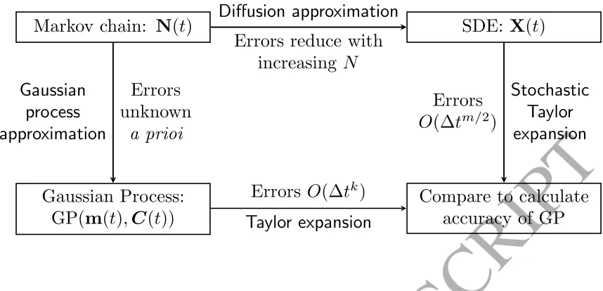
In this work, we present three main developments. First, we consider a very broad class of Gaussian process approximations, including those based on stochastic moment closure (which have branching process results as a special case) and those based on a linear time-inhomogeneous SDE (which have linear noise approximation approaches as a special case). Secondly, we give a method for deriving bounds on the errors of any Gaussian process approximation through Taylor expansion in the time interval between observations, using the scheme shown in Figure 1. Finally, we go into more depth than previously on the numerical comparison of different Gaussian process approximations for parameter inference on simulated data, and on how to apply these approaches to the data on cumulative incidence typically available from epidemiological outbreak reports.

2

Models and notation

While our approach is general, we will focus here on epidemic dynamics, in particular the Markovian SIR model, also called the general stochastic epidemic (Bailey, 1975; Andersson and Britton, 2000). We will define the different approaches as shown in Figure 1.

2.1 Pure jump Markov chain

We will write NS(t), NI(t) and NR(t) for the random integer numbers in the population who are

susceptible, infectious and removed respectively. The vector N(t) = (NS(t), NI(t), NR(t)) is then a

continuous-time Markov chain with events and rates

(NS, NI, NR)→(NS−1, NI+ 1, NR) at rateβ NSNI

N ,

(NS, NI, NR)→(NS, NI−1, NR+ 1) at rate γNI ,

(1)

where the population sizeN =NS+NI+NR is a constant.

2.2 Diffusion approximation

Using the convergence results of Kurtz (1970, 1971) the Markov chain defined by (1) is well approxi-mated by the solutionX(t) of the SDE

ACCEPTED MANUSCRIPT

where (ignoring the removed individuals who do not need to be counted due to the constant population size) we let

X(t) =

S(t)

I(t)

, F(X) =

−βSI/N βSI/N−γI

, V(X) =

βSI/N −βSI/N

−βSI/N βSI/N+γI

, (3)

and W =

W1 W2

where W1 and W2 are two independent Wiener processes. Explicitly, this

approxi-mation takes the form

NS ≈S , NI ≈I . (4)

Note that the distribution of X(∆t)|X(0) given by (2) will not in general be Gaussian.

2.3 Deterministic approximation

We can then further apply the results of Kurtz (1970, 1971) to derive the deterministic approximation

ds

dt =− β Nsi ,

di

dt = β

Nsi−γi, (5)

where s(t) and i(t) are the numbers of susceptible and infectious individuals respectively at time t

that satisfy this deterministic model.

2.4 Multivariate normal moment closure

For comparison, the multivariate normal (MVN) moment closure method is also used to obtain an approximation of the stochastic SIR model (Isham, 1991). In this method, it is assumed that the joint distribution of the susceptible and infectious populations can be approximated by a bivariate normal distribution. This gives a set of 5 ODEs for the mean and variances of the susceptible and infectious populations.

We write X(t) and Y(t) for the number of susceptible and infectious people respectively in the MVN moment closure approximation of the stochastic SIR model at timet. These follow a Gaussian process GP(µ(t),σ(t)) with mean and variance-covariance matrix

µ= µX µY =

E[X(t)] E[Y(t)]

, σ=

σXX σXY σXY σY Y

=

var(X(t)) cov(X(t), Y(t)) cov(X(t), Y(t)) var(Y(t))

, (6)

that obey equations

dµX

dt =− β

N(µXµY +σXY) ,

dµY

dt = β

N(µXµY +σXY)−γµY ,

dσXX

dt = β

N(µXµY +σXY −2µXσXY −2µYσXX) ,

dσXY

dt = β

N(µX(σXY −σY Y) +µY(σXX−σXY)−µXµY −σXY)−γσXY ,

dσY Y

dt = β

N(2µXσY Y + 2µYσXY +µXµY +σXY)−γ(2σY Y −µY) ,

(7)

ACCEPTED MANUSCRIPT

2.5 Linear stochastic process approximation

The linear stochastic process (LSP) approximation approach introduced in the SIR context by Isham (1991) (referring to a more complex model of AIDS due to Tan and Hsu (1989)) is to let the susceptible population evolve deterministically, while the infectious individuals are normally distributed.

This gives the following set of three ODEs for the evolution of the deterministic susceptible popu-lation,s(t), and the mean,µY =E[Y(t)], and variance,σY Y = var(Y(t)), of the infectious population:

ds

dt =− β NsµY ,

dµY

dt = β

NsµY −γµY ,

dσY Y

dt = β

N (2sσY Y +sµY)−γ(2σY Y −µY) .

(8)

While we mention this approach to show that various Gaussian moment closures are possible, for inferential purposes we will typically require the susceptible population to be random rather than deterministic making it unsuitable.

2.6 Linear SDE approximation

Following Archambeau et al. (2007), we note that the SDE

dx= (A(t)x+b(t)) dt+pU(t) dW , (9)

will have a Gaussian process solution GP(m(t),C(t)) with mean and variance-covariance matrix sat-isfying

dm

dt =Am+b ,

dC

dt =AC+CA

>_{+U . (10)}

Our aim is therefore to choose the time-varying matrices in equation (9) so that it approximates (2) and hence the full stochastic system. In this context, there is one ‘obvious’ choice for the matrixU(t):

U(t) =

(β/N)s(t)i(t) ₋(β/N)s(t)i(t)

−(β/N)s(t)i(t) (β/N)s(t)i(t) +γi(t)

. (11)

For the matrixA(t) and the vectorb(t), however, there are many choices that have the correct mean behaviour. We will consider how an existing approach in the literature (the Linear Noise model) is a special case of the linear SDE approach, and also introduce other special cases that we do not believe are named.

We write _X(t), _Y(t) for the number of susceptible and infectious people respectively in this ap-proximation of the stochastic SIR model at timet. These follow a Gaussian process GP(m(t),C(t)) with mean and variance-covariance matrix

m=

m1 m2

=

E[X(t)] E[_Y(t)]

, C =

C11 C21 C21 C22

=

var(X(t)) cov(X(t),Y(t)) cov(_X(t),_Y(t)) var(_Y(t))

. (12)

2.6.1 Linear noise approximation

To derive the linear noise (LN) approximation (Uhlenbeck and Ornstein, 1930; Black and McKane, 2010) we start with the SDE (2) and write

ACCEPTED MANUSCRIPT

where the quantities ˜S,I˜are assumed to be small in the approximation. Ignoring quadratic terms

O( ˜S2_,S˜_I,˜ _I˜2_{) and keeping only linear terms gives}

d

S(t)

I(t)

≈

−(β/N)(s(t)I(t) +S(t)i(t)₋s(t)i(t)) (β/N)(s(t)I(t) +S(t)i(t)₋s(t)i(t))₋γI(t)

dt

+

s

(β/N)s(t)i(t) −(β/N)s(t)i(t)

−(β/N)s(t)i(t) (β/N)s(t)i(t) +γi(t) dW .

(14)

This is a special case of the linear SDE approach where

A(t) =

−(β/N)i(t) ₋(β/N)s(t) (β/N)i(t) (β/N)s(t)−γ

; b(t) =

(β/N)s(t)i(t)

−(β/N)s(t)i(t)

. (15)

2.6.2 Other special cases

We consider two other special cases, which we name in an obvious way,

‘A noise’: A(t) =

−(β/N)i(t) 0 0 (β/N)s(t)₋γ

; b(t) =0 .

‘b noise’: A(t) =0 ; b(t) =

−(β/N)s(t)i(t) (β/N)s(t)i(t)−γi(t)

.

(16)

For each of these we obtain a set of five ODEs from (10), which we can solve numerically to give an approximation of the mean and variances of the stochastic SIR model. Note that there are more special cases, similar to these, for which we can write downA(t) and b(t).

2.7 Comparison of multivariate normal moment closure and linear SDE approxi-mations

The main difference between the MVN moment closure and linear SDE approaches is as follows. For the MVN moment closure, we have

dE[Y] dt =

β

N(E[X]E[Y] + cov(X, Y))−γE[Y] . (17)

For the linear SDE, in contrast, we have

dE[_Y] dt =

β

NE[X]E[Y]−γE[Y] . (18)

So the MVN moment closure allows for the negative correlation of the susceptibles and infecteds at the beginning (and end) of the outbreak. This means that E[Y] initially increases more slowly which allows for a random delay time before the outbreak takes off.

3

Numerical comparisons

ACCEPTED MANUSCRIPT

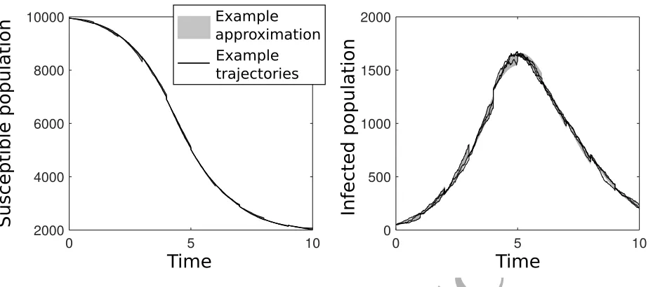
Figure 2 shows an example of these trajectories for a specific set of parameter values. Simulating 104 trajectories gives a distribution at each time point to which we compare each approximating Gaussian distribution.

For each approximation we computed the mean and variance of the size of the susceptible and infectious populations forward from the current data point until the next. The mean of the approxi-mation was then reset to the data point, and the variances to zero. Figure 2 shows an example of this for one specific set of parameter values and one specific approximation.

We compared the approximations numerically to the stochastic simulations using the Kullback-Leibler (KL) divergence, a measure of difference between two probability distributions. The Gaussian distributions of the approximations were discretised in order to compare with the discrete distribution given by the stochastic simulations. For discrete probability distributionsP andQthe KL divergence is defined as

DKL(P||Q) = X

i

P(i)(lnP(i)−lnQ(i)) . (19)

A better approximation results in a smaller KL divergence (MacKay, 2003). The KL divergence was computed each time data were obtained and before the simulations and approximations were reset to the data value.

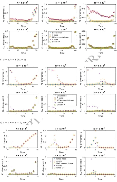
Note that we could not compute the KL divergence for a comparison of the LSP with the stochas-tic simulations for the size of the susceptible population as in the LSP the susceptible population evolves deterministically. Additionally, on occasion the KL divergence could not be computed for other approximations because one distribution took a value very close to zero. However, as displayed in Figure 3, this does not occur very often.

Figure 3 demonstrates these comparisons for three examples of epidemiological model rate pa-rameters that we have chosen to cover a range of R0 values. The MVN moment closure and LN

approximations consistently have the smallest KL divergence in both the size of the susceptible pop-ulation and the size of the infectious poppop-ulation (Figure 3). Additionally, and in particular for larger population sizes, the A noise and LSP approximations also approximate well the size of the infectious population. The b noise approximation does not approximate the size of the infectious class as well, in particular at the start and end of the epidemic.

For approximating the size of the susceptible population, the A noise and b noise approximations perform adequately but not as well as the other approximations particularly at the start and end of the epidemic.

We performed the same analysis over longer time steps, ∆t, and saw similar results; the MVN moment closure and LN approximations are best, with the A noise approximation also a good approx-imation for the infectious population. However, the A noise approxapprox-imation becomes a much less good approximation of the susceptible population over longer time steps.

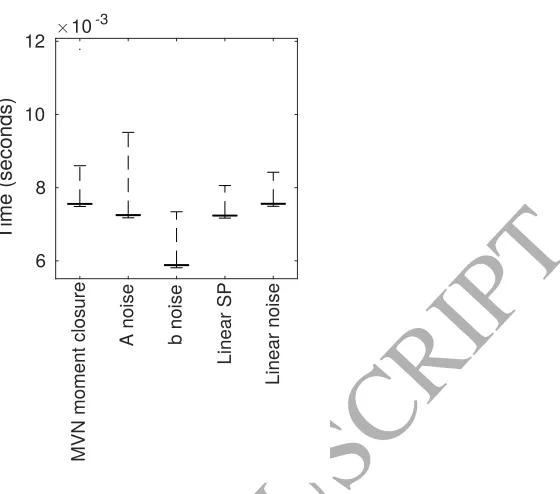
The ODEs that define the approximations were solved numerically. The b noise approximation has the simplest set of ODEs and so is fastest to solve. The A noise and LSP approximations are slower and, finally, the MVN moment closure and LN approximations take longest (Figure 4).

In addition, we note the ease with which the A noise and b noise approximations can be derived (in essence, just written down) in comparison to the MVN moment closure and LN approaches. This will become more pronounced for more complex compartmental models (for example, as demonstrated in section 5.2 when we apply these approximations to the SEIR model).

ACCEPTED MANUSCRIPT

We now consider what progress is possible analytically.

4

Analytical comparisons

Each of the Gaussian models previously described is chosen on the basis of differenta priori assump-tions, however we would like to find a way to control the errors introduced in a systematic manner. Since we are interested in regularly-spaced observations, the relevant control parameter is the timestep ∆t. Our starting point is the diffusion approximation to the stochastic SIR model in the regime where the susceptible population is approximately constant (e.g. atN when this is close to its starting value). This is chosen to simplify calculations, although we note the work of Cauchemez and Ferguson (2008) suggests that the approximation of constant susceptible population can be made throughout the epi-demic if the time period ∆t over which it is made is relatively small. In this limit, the system is described by the SDE first analysed by Feller (1951),

dI =rIdt+pρIdW , (20)

wherer =β₋γ andρ=β+γ. We will now consider how to expand this equation in ∆t.

4.1 Taylor scheme for SDEs

The origin of the methods used to derive Taylor schemes for SDEs is often attributed to Milstein (1975), who derived a scheme up to O(∆t). In fact, there are many such schemes that solve the SIR SDE locally in time; we use the weak order-3 scheme given by Kloeden and Platen (1992). This scheme has a rather complex general form, however for the specific equation (20) subject to initial condition

I(0) =I0 1 we obtain the following result following some analytical work:

I(∆t) =I0

1 +r∆t+ 1 2r

2_∆t2

+

ρI0∆t

1 +3 2r∆t+

7 6r

2_∆t2

1/2

U +O(∆t3, I00) , (21)

whereU ∼ N(0,1) is a standard normal random variable andO(∆t3, I00) represents terms containing

the variables ∆tn for n _≥ 3 and I₀m for m _≥ 0. Such a stochastic Taylor expansion can be carried out for any SDE, including multi-dimensional ones, and as such we believe this method has significant promise for evaluation of Gaussian process approximations in general. While the complexity of analysis can grow, it is possible to work with such stochastic systems using computer algebra (Kendall, 2005), and we think that this would be an interesting direction for future research.

4.2 Local solution of ODEs giving the approximations

For the Gaussian process approximations that arise from linear SDEs, we consider (10) in the limit where the size of the susceptible population is approximately constant to give the following ODEs for the mean,m2, and variance,C22, of the number of infecteds,

dm2

dt =A21(t)N+A22(t)m2(t) +b2(t) ,

dC22

dt = 2A22(t)C22(t) +ρi(t) .

(22)

Solving these, using a standard Taylor series expansion subject to initial conditionsm2(0) =i(0) =I0

and C22(0) = 0, gives for each considered model

m2(∆t) =I0

1 +r∆t+1 2r

2_∆t2_{+· · ·}

ACCEPTED MANUSCRIPT

i.e. as we would expect the Taylor series for er∆t. For b noise, we have

C22(∆t) =ρI0

1 +1 2r∆t+

1 6r

2_∆t2_{+· · ·}

∆t, (24)

where for all other models (A noise and LN) we have

C22(∆t) =ρI0

1 +3 2r∆t+

7 6r

2_∆t2_{+· · ·}

∆t. (25)

For the MVN moment closure approximation, the mean,µY(t), and variance, σY Y, of the epidemic at

constant susceptible population are given by the following ODEs:

dµY

dt =rµY,

dσY Y

dt =ρµY + 2rσY Y,

(26)

which we can also solve subject toµY =I0,σY Y = 0 to obtain

µY(∆t) =I0

1 +r∆t+1 2r

2_∆t2_{+· · ·}

,

σY Y(∆t) =ρI0

1 +3 2r∆t+

7 6r

2_∆t2_{+· · ·}

∆t.

(27)

4.3 Bounding the errors of the Gaussian process

Putting the results above together, we see that the MVN moment closure, linear noise and A noise are all consistent with the SDE (20) expanded as in equation (21), so we will continue to work with these approaches, while the b noise is significantly less accurate and so we do not consider it further. To see why errors at this order represent a significant improvement on other possible approaches, consider the Euler-Maruyama approximation to (20),

J(∆t) = (1 +r∆t)I0+ p

ρI0∆tU , (28)

whereU is a standard Gaussian random variable. Comparing to (21) we see that errors to this appear atO(∆t). This tells us that the ODE-based Gaussian process approximations we continue to analyse (MVN, LN and A) are more accurate than Euler-Maruyama steps by several orders of magnitude in ∆t.

5

Inference

ACCEPTED MANUSCRIPT

5.1 Simulated data from the SIR model

Consider a disease that is well approximated by the SIR model with transmission rate constant β

and recovery rate constant γ. Suppose we have data of the form of a set of times _{ti}ni=0 together

with associated measurements of the number of infecteds _{yi}ni=0. Consider a Gaussian process

ap-proximation to the SIR model such that given susceptible and infectious populations of sizex0 and y0

respectively at the start of a time interval of length ∆t, at the end of that time interval the mean and variance-covariance matrix are µ(∆t;x0, y0, β, γ) and Σ(∆t;x0, y0, β, γ) respectively. If we also had

measurements of the susceptible population,{xi}n_i=0, then we could write the likelihood function for

the parameters of the approximating model given the data as

L(β, γ;x,y) =

n Y

i=1

N ((xi, yi);µ(ti−ti−1;xi−1, yi−1, β, γ),Σ(ti−ti−1;xi−1, yi−1, β, γ)) . (29)

In practice, the data on the susceptible population are not readily available and instead this information can be imputed using the marginal and marginal conditional distributions of a multivariate normal distribution. These can be explicitly computed as follows (Eaton, 1983). For random vector (x, y) with multivariate normal distributionN(µ,Σ) an observationyi has marginal probability density function

f(yi) =N(yi;µ2,Σ22) , (30)

and conditional on this observation xi has marginal conditional probability density function

f(xi;yi) =N(xi;µ1+ Σ12Σ−221(yi−µ2),Σ11−Σ12Σ−221Σ21) . (31)

We can use these rules at each observation point to build up a likelihood from the product of terms such as (30) and also to update the mean vector and variance-covariance matrix for the Gaussian process approximation.

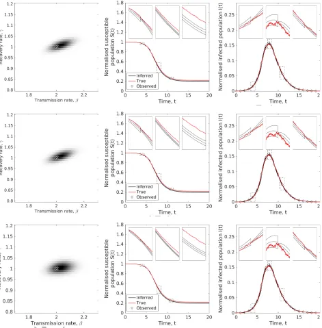
Synthetic data were obtained from one simulation of the stochastic SIR model using parameter values β = 2, γ = 1, and N = 1×104 with one initial infected. Using each of the MVN moment closure, LN, and A noise approximations, we were reliably able to recover the epidemiological model parameters as shown in Figure 5. The three approximation methods all gave similar results for parameter estimates (estimates ˆβ= 2.04 and ˆγ = 1.01) and for the size of the susceptible population from regular data on the number of infecteds.

5.2 Cumulative incidence from a real norovirus outbreak with the SEIR model

In the previous section we discussed the case when the available data are the number of infecteds at regular time points. An alternative, and common, situation is when only illness onset times, and not recovery times are available. For an SIR model this corresponds to having measurements of the

cumulative incidence N₋S(t).

ACCEPTED MANUSCRIPT

by dX=F(X) dt+pV(X) dW with

X(t) =

 ES((tt))

I(t)



 , F(X) =



βSI/N−βSI/N−ωE ωE₋γI

  ,

V(X) =

 

βSI/N ₋βSI/N 0

−βSI/N βSI/N+ωE −ωE

0 ₋ωE ωE+γI   .

(32)

The deterministic approximation of the stochastic SEIR model is given by the ODEs

ds

dt =− β Nsi,

de

dt = β

Nsi−ωe

di

dt =ωe−γi , (33)

where, as before,s(t),e(t), andi(t) are the numbers of susceptible, exposed, and infected individuals respectively at timet given by the deterministic model.

To use the linear SDE Gaussian process approximation with the SEIR model we simply need again to choose the time-varying matrices in (9) so that it approximates (32). For the A noise approximation introduced in this work this will be

A(t) =

 

0 0 ₋βs(t)/N

0 ₋ω βs(t)/N

0 ω −γ 

 , b(t) =

  0 0 0   ,

U(t) =

 

βs(t)i(t)/N ₋βs(t)i(t)/N 0

−βs(t)i(t)/N βs(t)i(t)/N +ωe(t) ₋ωe(t) 0 −ωe(t) ωe(t) +γi(t)

  .

(34)

As before, we can infer the unobserved time seriesE(t) andI(t) using the general conditional laws of Gaussian processes (Rasmussen and Williams, 2005), and use the marginal laws to perform maximum likelihood estimation on the parameter values β,γ, and S(0). Note that we fitS(0) instead of taking it to be N ₋1 because we do not know the infection history of the population. For example, some of the population may have been previously recently exposed to norovirus and therefore not currently susceptible. We make the somewhat conservative assumption that newly diagnosed individuals are no longer susceptible but could potentially be in any of theE,I, orRstates so that our data are effectively values ofN ₋S(t) – a different approach could easily be taken within our inferential framework.

Additionally, some care must be taken because ω is poorly identifiable from this cumulative inci-dence data, and our attempts to fit it alongside the other three parameters produced unrealistically large estimates motivating us to fix this parameter from other data. We found that the literature gives the latent, or incubation, period of norovirus to be between 0.5 and 2 days. For example, an SEIR model fitted to an outbreak in a long-term care facility estimated the latent period of norovirus as 1.3 days (Vanderpas et al., 2009). A systematic review of the incubation period of norovirus genogroups I and II gives it as 1.2 days (95% confidence interval 1.1–1.2) (Lee et al., 2013). The CDC report that the incubation period of norovirus is between 0.5 and 2 days (Centers for Disease Control and Prevention, 2011). Finally, a large dataset of norovirus outbreaks showed the incubation period to have a mean and median of 1.4 (95% confidence interval 1.3–1.4) days. Sinceωis the reciprocal of the latent period, we therefore choseω= 2 days−1 as the largest value consistent with existing knowledge about norovirus.

Working at two significant figures or zero decimal places as appropriate, parameter estimates and 95% confidence intervals from fitting the data with the MVN moment closure approximation are:

ACCEPTED MANUSCRIPT

confidence intervals from fitting the data with the LN approximation are: β _≈ 18 [8.6,27], γ _≈ 1.1 [0,3.1] days−1_{, andS}

0≈237 [137,336]. Parameter estimates and 95% confidence intervals from fitting

the data with the A noise approximation are: β ≈23 [0.81,44], γ ≈1.5 [0,4.7] days−1, and S0 ≈241

[125,357]. These confidence intervals are truncated at zero for rate parameters. The standard error estimates for the intervals were taken from the leading diagonal of an approximate covariance matrix of the parameter estimates. The approximate covariance matrices were computed as the negative inverse of an approximation to the Hessian of the log-likelihood at the maximum likelihood estimates obtained using finite differences (from the MATLAB function mlecov()). The correlation matrices between the parameters for each approach are, respectively,

RMVN= 

10..00 077 1..77 000 0..3787 0.37 0.87 1.00



 , RLN = 

10..00 079 1..79 000 0..5794 0.57 0.94 1.00



 , RA=



10..00 091 1..91 000 0..7193 0.71 0.93 1.00



 . (35)

Our overall picture, as would be expected when fitting a complex non-linear stochastic model to limited data, is of highly correlated parameters with relatively large marginal confidence intervals. The average infectious periods (estimated from 1/γ as 0.59, 0.91, and 0.67 days for the MVN moment closure, LN, and A noise approximations respectively) are shorter than the natural history of norovirus would indicate, which is likely to be due to control measures in place upon the ship (Vivancos et al., 2010) limiting the time period during which cases are able to infect others. Additionally, S(0) is estimated as much smaller thanN, which could be due to pre-existing immunity, control measures in place on board the ship, and non-homogeneous mixing (through excursion choice and cabin location) (Vivancos et al., 2010).

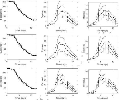
Results for learning the time series of S(t), E(t) and I(t) are shown in Figure 6, which shows general agreement on mean behaviour, but differences in the uncertainty.

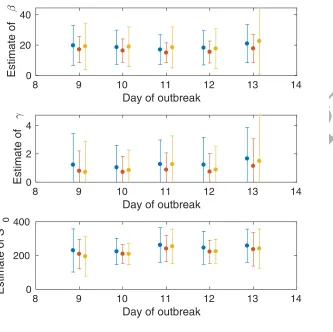
In the results presented so far, the full dataset has been used to estimate the parameters of the epidemic model, before the time series were estimated as the epidemic progressed. We show here, in Figure 7, the results of also estimatingβ, γ, and S0 as the epidemic progressed, beginning from day

nine. Note that in this instance, these methods did not work with fewer than nine days of data. These datapoint-by-datapoint estimates remain consistent over the epidemic.

We conclude that even in this common case where there is a small dataset of symptom onset times, our Gaussian process approach can be applied and gives epidemiologically reasonable answers in little computational time.

6

Conclusions

In this paper, we have sought to provide results that will allow Gaussian process approximation to become a more routinely used technique in infectious disease epidemiology. We have considered a wide class of Gaussian process approximations, as well as methods to bound the errors on the use of these. We have compared these using simulated data and applied them to real data. For future work, we would like to address the methodological challenges that face infectious disease epidemiologists and the public health system such as inaccuracy in case ascertainment, the requirement for analysis methods to be online in real-time and robust, and the ability to make predictions going forward under uncertainty.

Conflicts of interest

ACCEPTED MANUSCRIPT

Acknowledgements

EBJ and TH are supported by the Engineering and Physical Sciences Research Council (Grant numbers EP/I01358X/1 and EP/N033701/1). We would like to thank the International Centre for Mathemat-ical Sciences in Edinburgh for hosting us while we developed this work and also the participants in the ‘Stochastic models of the spread of disease and information on networks’ workshop for helpful comments on it. We would also like to thank the two anonymous referees for their constructive input.

References

H. Andersson and T. Britton. Stochastic Epidemic Models and Their Statistical Analysis. Springer, Lecture Notes in Statistics, Vol. 151, 2000.

C. Andrieu, A. Doucet, and R. Holenstein. Particle Markov chain Monte Carlo methods. Journal of the Royal Statistical Society: Series B (Statistical Methodology), 72(3):269–342, 2010.

C. Archambeau, D. Cornford, M. Opper, and J. Shawe-taylor. Gaussian process approximations of stochastic differential equations. Journal of Machine Learning Research: Workshop and Conference Proceedings, 1:1–16, 2007.

N. T. J. Bailey. The mathematical theory of infectious diseases and its applications. 2nd edition.

Griffin, London, 1975.

F. Ball and T. House. Heterogeneous network epidemics: real-time growth, variance and ex-tinction of infection. Journal of Mathematical Biology, pages Published online ahead of print, DOI:10.1007/s00285–016–1092–3, 2017.

A. J. Black and A. J. McKane. Stochastic amplification in an epidemic model with seasonal forcing.

Journal of Theoretical Biology, 267(1):85–94, 2010.

S. Cauchemez and N. M. Ferguson. Likelihood-based estimation of continuous-time epidemic models from time-series data: application to measles transmission in London. Journal of The Royal Society Interface, 5(25):885–897, 2008.

Centers for Disease Control and Prevention. Updated norovirus outbreak management and disease prevention guidelines. Morbidity and Mortality Weekly Report (MMWR), 60(4):1–18, 2011.

N. Chopin, P. E. Jacob, and O. Papaspiliopoulos. SMC2_{: an efficient algorithm for sequential analysis}

of state space models. Journal of the Royal Statistical Society: Series B (Statistical Methodology), 75(3):397–426, 2013.

C. Dargatz. Bayesian Inference for Diffusion Processes with Applications in Life Sciences. PhD thesis, Ludwig-Maximilians-Universit¨at, Munich, 2010.

M. L. Eaton. Multivariate Statistics: a Vector Space Approach. John Wiley and Sons, 1983.

P. Fearnhead, V. Giagos, and C. Sherlock. Inference for reaction networks using the linear noise approximation. Biometrics, 70(2):457–466, 2014.

W. Feller. Two singular diffusion problems. Annals of Mathematics, 54(1):173–182, 1951.

ACCEPTED MANUSCRIPT

R. Guy, C. Lar´edo, and E. Vergu. Approximation of epidemic models by diffusion processes and their statistical inference. Journal of Mathematical Biology, 70(3):621–646, 2015.

T. House. For principled model fitting in mathematical biology. Journal of Mathematical Biology, 70 (5):1007–1013, 2015.

E. L. Ionides, C. Bret´o, and A. A. King. Inference for nonlinear dynamical systems. Proceedings of the National Academy of Sciences, 103(49):18438–18443, 2006.

V. Isham. Assessing the variability of stochastic epidemics. Mathematical biosciences, 107(2):209–224, 1991.

W. S. Kendall. Stochastic integrals and their expectations. The Mathematica Journal, 9(4):757–767, 2005.

A. A. King, M. Domenech de Cell`es, F. M. G. Magpantay, and P. Rohani. Avoidable errors in the modelling of outbreaks of emerging pathogens, with special reference to Ebola. Proceedings of the Royal Society of London B: Biological Sciences, 282(1806), 2015.

P. E. Kloeden and E. Platen. Numerical Solution of Stochastic Differential Equations. Stochastic Modelling and Applied Probability. Springer-Verlag Berlin Heidelberg, 1992.

T. G. Kurtz. Solutions of ordinary differential equations as limits of pure jump Markov processes.

Journal of Applied Probability, 7(1):49–58, 1970.

T. G. Kurtz. Limit theorems for sequences of jump Markov processes approximating ordinary differ-ential processes. Journal of Applied Probability, 8(2):344–356, 1971.

J. Leander, T. Lundh, and M. Jirstrand. Stochastic differential equations as a tool to regularize the parameter estimation problem for continuous time dynamical systems given discrete time measure-ments. Mathematical Biosciences, 251:54–62, 2014.

R. M. Lee, J. Lessler, R. A. Lee, K. E. Rudolph, N. G. Reich, T. M. Perl, and D. A. T. Cummings. Incubation periods of viral gastroenteritis: a systematic review. BMC Infectious Diseases, 13(1): 446, 2013.

S. C. Leite and R. J. Williams. A constrained Langevin approximation for chemical reaction networks. Preprint available at _{http://www.math.ucsd.edu/~williams/biochem/biochem.html}, 2017.

D. J. MacKay. Information Theory, Inference, and Learning Algorithms. Cambridge University Press, 2003.

T. J. McKinley, J. V. Ross, R. Deardon, and A. R. Cook. Simulation-based Bayesian inference for epidemic models. Computational Statistics and Data Analysis, 71:434–447, 2014.

G. N. Milstein. Approximate integration of stochastic differential equations. Theory of Probability and its Applications, 19(3):557–562, 1975.

P. Neal and C. L. Terry Huang. Forward simulation markov chain monte carlo with applications to stochastic epidemic models. Scandinavian Journal of Statistics, 42(2):378–396, 2015.

ACCEPTED MANUSCRIPT

C. E. Rasmussen and C. K. I. Williams. Gaussian Processes for Machine Learning (Adaptive Compu-tation and Machine Learning). The MIT Press, Cambridge, Massachusetts, 2005.

J. V. Ross, T. Taimre, and P. K. Pollett. On parameter estimation in population models. Theoretical Population Biology, 70(4):498–510, 2006.

K. Simmons, M. Gambhir, J. Leon, and B. Lopman. Duration of immunity to norovirus gastroenteritis.

Emerging Infectious Diseases, 19:12601267, 2013.

W. Y. Tan and H. Hsu. Some stochastic models of AIDS spread. Statistics in Medicine, 8(1):121–136, 1989.

T. Toni, D. Welch, N. Strelkowa, A. Ipsen, and M. P. Stumpf. Approximate Bayesian computation scheme for parameter inference and model selection in dynamical systems. Journal of The Royal Society Interface, 6(31):187–202, 2009.

G. E. Uhlenbeck and L. S. Ornstein. On the theory of the brownian motion. Physical Review, 36(5): 823–841, 1930.

J. Vanderpas, J. Louis, M. Reynders, G. Mascart, and O. Vandenberg. Mathematical model for the control of nosocomial norovirus. Journal of Hospital Infection, 71(3):214–222, 2009.

R. Vivancos, A. Keenan, W. Sopwith, K. Smith, C. Quigley, K. Mutton, E. Dardamissis, G. Nichols, J. Harris, C. Gallimore, L. Verhoef, Q. Syed, and J. Reid. Norovirus outbreak in a cruise ship sailing around the British Isles: Investigation and multi-agency management of an international outbreak.

Journal of Infection, 60:478–485, 2010.

ACCEPTED MANUSCRIPT

Markov chain:

N

(

t

)

SDE:

X

(

t

)

Gaussian Process:

GP(

m

(

t

)

,

C

(

t

))

Compare to calculate

accuracy of GP

Gaussian

process

approximation

Errors

unknown

a prioi

Errors reduce with

increasing

N

Diffusion approximation

Taylor expansion

Errors

O

(∆

t

)

Stochastic

Taylor

expansion

Errors

O

(∆

t

)

ACCEPTED MANUSCRIPT

0 5 10

0 500 1000 1500 2000

0 5 10

2000 4000 6000 8000 10000

Time

Time

Example approximation Example trajectories

Suscept

ible population

Infected popu

lation

Figure 2: A typical example of stochastic trajectories and one Gaussian process approximation. This example was generated with parameters β = 2, γ = 1, and N = 1_×104 _{and the multivariate normal}

ACCEPTED MANUSCRIPT

0 10 20 30

Time 0

0.5

KL divergence: S

0 10 20 30

Time 0

0.2 0.4 0.6

KL divergence: I

N = 1 x 104

0 20 40

Time 0

0.2 0.4

KL divergence: S

0 20 40

Time 0 0.1 0.2 0.3 0.4

KL divergence: I

N = 1 x 105

Linear noise A noise

MVN moment closure b noise

Linear SP

0 20 40

Time 0

0.05 0.1

KL divergence: S

0 20 40

Time 0 0.02 0.04 0.06 0.08

KL divergence: I

N = 1 x 106

(b)β= 2,γ= 1 (R0= 2)

0 5 10 15

Time 0 0.5 1 1.5 2

KL divergence: S

N = 1 x 104

0 5 10 15

Time

0 0.5 1

KL divergence: I

N = 1 x 104

0 5 10 15

Time 0 0.5 1 1.5 2

KL divergence: S

N = 1 x 105

0 5 10 15

Time

0 0.5 1

KL divergence: I

N = 1 x 105

Linear noise A noise

MVN moment closure b noise

Linear SP

0 5 10 15

Time 0 0.5 1 1.5 2

KL divergence: S

N = 1 x 106

0 5 10 15

Time

0 0.5 1

KL divergence: I

N = 1 x 106

(c)β= 3,γ= 0.5 (R0= 6)

0 5 10 15

Time

0 1 2 3

KL divergence: S

N = 1 x 104

0 5 10 15

Time 0 0.2 0.4 0.6 0.8

KL divergence: I

N = 1 x 104

0 5 10 15

Time

0 0.5 1 1.5

KL divergence: S

N = 1 x 105

0 5 10 15

Time

0 2 4 6

KL divergence: I

N = 1 x 105

Linear noise A noise

MVN moment closure b noise

Linear SP

0 5 10 15

Time

0 5 10

KL divergence: S

N = 1 x 106

0 5 10 15

Time 0 5 10 15 20

KL divergence: I

N = 1 x 106

Figure 3: Numerical comparisons of the approximation schemes with stochastic simulations of the SIR model using the KL divergence. Within each subplot (a-c) different rate constant parameter values were used to generate stochastic simulations for comparison to each Gaussian approximation. The size of the susceptible population is compared on the top line and the size of the infectious population

ACCEPTED MANUSCRIPT

MVN moment closure

A noise b noise

Linear SP

Linear noise

6 8 10 12

Time (seconds)

10-3

MVN moment closure

A noise b noise

Linear SP

Linear noise

MVN moment closure

A noise b noise

Linear SP

Linear noise

MVN moment closure

A noise b noise

Linear SP

Linear noise

MVN moment closure

A noise b noise

Linear SP

Linear noise

ACCEPTED MANUSCRIPT

ACCEPTED MANUSCRIPT

0 5 10

Time (days) 0 50 100 150 200 250 Susceptible

0 5 10

Time (days) 0 5 10 15 20 25 Exposed

0 5 10

Time (days) 0 5 10 15 20 25 Infectious

0 5 10

Time (days) 0 50 100 150 200 Susceptible

0 5 10

Time (days) 0 5 10 15 20 25 Exposed

0 5 10

Time (days) 0 10 20 30 Infectious

0 5 10

Time (days) 0 50 100 150 200 Susceptible

0 5 10

Time (days) 0 5 10 15 20 25 Exposed

0 5 10

Time (days) 0 10 20 30 Infectious

ACCEPTED MANUSCRIPT

Day of outbreak

0 20 40

Estimate of

8 9 10 11 12 13 14

Day of outbreak

0 2 4

Estimate of

8 9 10 11 12 13 14

Day of outbreak

0 200 400

Estimate of S

0

Figure 7: Estimates of the model parameters β, γ, and S0 as the epidemic progresses for the