A computationally efficient nonparametric approach for
changepoint detection
Kaylea Haynes
1†, Paul Fearnhead
2and Idris A. Eckley
31
STOR-i Centre for Doctoral Training, Lancaster University
2
Department of Mathematics and Statistics, Lancaster University
†
Correspondence: [email protected]
Abstract
In this paper we build on an approach proposed by Zou et al. (2014) for
nonpara-metric changepoint detection. This approach defines the best segmentation for a data
set as the one which minimises a penalised cost function, with the cost function defined
in term of minus a non-parametric log-likelihood for data within each segment.
Min-imising this cost function is possible using dynamic programming, but their algorithm
had a computational cost that is cubic in the length of the data set. To speed up
computation, Zou et al. (2014) resorted to a screening procedure which means that the
estimated segmentation is no longer guaranteed to be the global minimum of the cost
function. We show that the screening procedure adversely affects the accuracy of the
changepoint detection method, and show how a faster dynamic programming algorithm,
Pruned Exact Linear Time, PELT (Killick et al., 2012), can be used to find the optimal
segmentation with a computational cost that can be close to linear in the amount of
data. PELT requires a penalty to avoid under/over-fitting the model which can have a
detrimental effect on the quality of the detected changepoints. To overcome this issue
we use a relatively new method, Changepoints Over a Range of PenaltieS (CROPS)
(Haynes et al., 2015), which finds all of the optimal segmentations for multiple penalty
values over a continuous range. We apply our method to detect changes in heart rate
Keywords: nonparametric maximum likelihood, PELT, CROPS, activity tracking
1
Introduction
Changepoint detection is an area of statistics broadly studied across many disciplines such
as acoustics (Guarnaccia et al., 2015; Lu and Zhang, 2002), genomics (Olshen et al., 2004;
Zhang and Siegmund, 2007) and oceanography (Nam et al., 2014). Whilst the changepoint
literature is vast, many existing methods are parametric. For example a common approach is
to introduce a model for the data within a segment, use minus the maximum of the resulting
log-likelihood to define a cost for a segment, and then define a cost of a segmentation as the
sum of the costs for each of its segments. See for example Yao (1988); Lavielle (2005); Killick
et al. (2012); Davis et al. (2006). Finally, the segmentation of the data is obtained as the one
that minimises a penalised version of this cost (see also Frick et al., 2014, for an extension
of these approaches).
A second class of methods are based on tests for a single changepoint, with the tests often
defined based on the type of change that is expected (such as change in mean), and the
distribution of the null-statistic for each test depending on further modelling assumptions for
the data (see e.g. Bai and Perron, 1998; Dette and Wied, 2015). Tests for detecting a single
change can then be applied recursively to detect multiple changes, for example using binary
segmentation (Scott and Knott, 1974) or its variants (e.g. Fryzlewicz, 2014). For a review of
alternative approaches for change detection see Jandhyala et al. (2013) and Aue and Horvth
(2013).
Much of the existing literature on nonparametric methods look at single changepoint
detec-tion (Page, 1954; Bhattacharyya and Johnson, 1968; Carlstein, 1988; Dumbgen, 1991).
Sev-eral approaches are based on using rank statistics such as the Mann-Whitney test statistic
(Pettitt, 1979). Ross and Adams (2012) introduce the idea of using the Kolmogorov-Smirnov
and the Cramer-von Mises test statistics; both of which use the empirical distribution
func-tion. Other methods include using kernel density estimations (Baron, 2000), however these
can be computationally expensive to calculate.
change-point detection methods which have been developed using nonparametric methods do not
extend easily to multiple changepoints. Within the sequential changepoint detection
litera-ture one can treat the problem as a single changepoint problem which resets every time a
changepoint is detected (Ross and Adams, 2012). Lee (1996) proposed a weighted empirical
measure which is simple to use but has been shown to have unsatisfactory results. Under the
multivariate setting Matteson and James (2013) proposed methods, E-divisive and e-cp3o,
based on clustering and probabilistic pruning respectively. The E-divisive method uses an
exact test statistic with an approximate search algorithm whereas the e-cp3o method uses
an approximate test statistic with an exact search algorithm. As a result e-cp3o is faster but
lacks slightly in the quality for the changepoints detected.
In this article we focus on univariate changepoint detection and we are interested in the
work of Zou et al. (2014) who propose a nonparametric likelihood based on the empirical
distribution. They then use a dynamic programming approach, Segment Neighbourhood
Search (Auger and Lawrence, 1989), which is an exact search procedure, to find multiple
changepoints. Whilst this method is shown to perform well, it has a computational cost of
O(M n2+n3) where M is the number of changepoints and n is the length of the data. This
makes this method infeasible when we have large data sets, particularly in situations where
the number of changepoints increases with n. To overcome this, Zou et al. (2014) propose
an additional screening step that prunes many possible changepoint locations. However, as
we establish in this article, this screening step can adversely affect the accuracy of the final
inferred segmentation.
In this paper we seek to develop a computationally efficient approach to the multiple
change-point search problem in the nonparametric setting. Our approach is an extension to the
method of Zou et al. (2014). This firstly involves simplifying the definition of the segment
cost, so that calculating the cost for a given segment involves computation that is O(logn)
rather than O(n). Secondly we apply a different dynamic programming approach, Pruned
Exact Linear Time (PELT) (Killick et al., 2012), that is substantially quicker than Segment
Neighbourhood Search; for many situations where the number of changepoints increases
lin-early with n, PELT has been proven to have a computational cost that is linear in n.
is penalised. The quality of the final segmentation can be sensitive to this choice, and
whilst there are default choices these do not always work well. However we show that the
Changepoints for a Range of PenaltieS (CROPS) algorithm (Haynes et al., 2015) can be used
with NP-PELT to explore optimal segmentations for a range of penalties.
The rest of this paper is organised as follows. In Section 2 we give details of the NMCD
approach proposed by Zou et al. (2014). In Section 3 we introduce our new efficient
nonpara-metric search approach, nonparanonpara-metric PELT (NP-PELT) and show how we can substantially
improve the computational cost of this method. In Section 4 we demonstrate the performance
of our method on simulated data sets comparing our method with NMCD. Finally in Section
5 we include some simulations which analyse the performance of NMCD for different
sce-narios and then we show how a nonparametric cost function can be beneficial in situations
where we do not know the underlying distribution of the data. In order to demonstrate our
method we use heart rate data recorded whilst an individual is running.
2
Nonparametric Changepoint Detection
2.1
Model
The model that we refer to throughout this paper is as follows. Assume that we have data,
x1, ..., xn∈R , that have been ordered based on some covariate information such as time or
position along a chromosome. For v ≥uwe denote xu:v ={xu, ..., xv}. Throughout we letm
be the number of changepoints, and the positions beτ1, . . . , τm. Furthermore we assume that
τi is an integer and that 0 =τ0 < τ1 < τ2 < ... < τm < τm+1 =n. Thus our m changepoints
split the data into m+ 1 segments, with the ith segment containing xτi−1+1:τi.
As in Zou et al. (2014) we will let Fi(t) be the (unknown) cumulative distribution function
(CDF) for the ith segment, and ˆFi(t) the empirial CDF. In other words
ˆ
Fi(t) =
1
τi−τi−1 ×
τi
X
j=τi−1+1
1{xj < t}+ 0.5×1{xj =t}
. (2.1)
2.2
Nonparametric maximum likelihood
If we have n data points that are independent and identically distributed with CDF F(t),
then, for a fixed value of t, the empirical CDF will satisfy nFˆ(t)∼Binomial(n, F(t)). Hence
the log-likelihood of F(t) is given by: n{Fˆ(t) log(F(t)) + (1−Fˆ(t)) log(1−F(t))}. This
log-likelihood is maximised by the value of the empirical CDF, ˆF(t). We can thus use minus the
maximum value of this log-likelihood as a segment cost function. So for segment i we have
a cost that is −Lnp(xτi−1+1:τi;t) where
Lnp(xτi−1+1:τi;t) = (τi−τi−1)×[ ˆFi(t) log ˆFi(t) + (1−Fˆi(t)) log(1−Fˆi(t))]. (2.2)
We can then define a cost of a segmentation as the sum of the segment costs. Thus to segment
the data with m changepoints we minimise −Pm+1i=1 Lnp(xτi−1+1:τi;t).
2.3
Nonparametric multiple changepoint detection
One problem with the segment cost as defined by (2.2) is that it only uses information about
the CDF evaluated at one value of t and that the choice of t can have detrimental effects on
the resulting segmentations. To overcome this Zou et al. (2014) suggest defining a segment
cost which integrates (2.2) over different values of t. They suggest a cost function for a
segment with data xu:v that is
Z ∞
−∞−L
np(xu:v;t)dw(t), (2.3)
with a weight, dw(t) ={F(t)(1−F(t))}−1dF(t), that depends on the CDF of the full data.
This weight is chosen to produce a powerful goodness of fit test (Zhang, 2002). As this
is unknown they approximate it by the empirical CDF of the full data, and then further
approximate the integral by a sum over the data points. This gives the following objective
function
QNMCD(τ1:m;x1:n) = −n m+1X
i=1 n
X
t=1
(τi−τi−1)×
ˆ
Fi(t) log ˆFi(t) + (1−Fˆi(t)) log(1−Fˆi(t))
(t−0.5)(n−t+ 0.5) .
For a fixed m this objective function is minimised to find the optimal segmentation of the
data.
In practice a suitable choice of m is unknown, and Zou et al. (2014) suggest estimating m
using the Schwarz’ Information criterion (Schwarz, 1978). That is, they minimise
SIC = min
m;τ1,...,τm{
QNMCD(τ1:m;x1:n) +mξn}, (2.5)
where ξn is a sequence going to infinity.
2.4
NMCD Algorithm
To maximise the objective function (2.4), Zou et al. (2014) use the dynamic programming
algorithm Segment Neighbourhood Search (Auger and Lawrence, 1989). This algorithm
calculates the optimal segmentations, given a cost function, for each value of m= 1, . . . , M,
where M is a specified maximum number of changepoints to search for. If all the segment
costs have been pre-computed then Segment Neighbourhood search has a computational cost
of O(M n2). However for NMCD the segment cost involves calculating
n
X
t=1
ˆ
Fi(t) log ˆFi(t) + (1−Fˆi(t)) log(1−Fˆi(t))
(t−0.5)(n−t+ 0.5) ,
and thus calculating the cost for a single segment is O(n). Hence the cost of precomputing
all segment costs is O(n3), and the resulting algorithm has a cost that is O(M n2+n3).
To reduce the computational burden when we have long data series, Zou et al. (2014) propose
a screening step. They consider overlapping windows of length 2NI for some NI ∈ R. For
each window they calculate the Cram´er-von Mises (CvM) statistic for a changepoint at the
centre of the window. They then compare these CvM statistics, each corresponding to a
different changepoint location, and remove a location as a candidate changepoint if its CvM
statistic is smaller than any of the CvM statistics for locations within NI of it. The number
of remaining candidate changepoint positions is normally much smaller than n and thus
the computational complexity can be substantially reduced. The choice of NI is obviously
but at the risk or removing true changepoint locations. In particular, the rationale for the
method is based onNI being smaller than any segment that you wish to detect. As a default,
Zou et al. (2014) recommend choosing NI = d(logn)3/2/2e where dxe denotes the smallest
integer which is larger than x.
3
NP-PELT
Here we develop a new, computationally efficient, way to segment data using a cost function
based on (2.3). This involves firstly an alternative numerical approximation to the integral
(2.3), which is more efficient to calculate. In addition we use a more efficient dynamic
programming algorithm, PELT (Killick et al., 2012), to then minimise the cost function.
3.1
Improved Segment Cost
To reduce the cost of calculating the segment cost, we approximate the integral by a sum
with K << n terms. The integral in (2.3) involves a weight, and we first make a change of
variables to remove this weight.
Lemma 3.1. Let c=−log(2n−1). For x∈[−1,1] define p(x) = (1 + exp{cx})−1. Then
Z 2n−1
2n
1 2n
Lnp(xu:v;t){F(t)(1−F(t))}−1dF(t) =−c
Z 1
−1L
np(xu:v;F−1(p(x)))dx. (3.1)
Proof. This follows from making the change of variable F(t) =p(x).
Using Lemma 3.1, we suggest the following approximation, based on an approximation of
(3.1) usingK evenly spacedx-values. FixK, and defineγ such thatK =c/γ, with cdefined
as in Lemma 3.1. Lett1, . . . , tKbe such thattkis the (1+(2n−1) exp{γ(2k−1)})−1 empirical
quantile of the data, then we approximate (2.3) by
CK(xu:v) = −
2c K
K
X
The idea is that (2.3) gives higher weight to values of t in the tail of the distribution of the
data. Our approximation achieves this through a sum where each term has equal weight, but
where the tk values we choose are prefentially chosen from the tail of the distribution.
The cost now for calculating the segment costs is O(K). If we choose K =dc/γe, where cis
defined in Lemma 3.1, for some fixed γ then this will be O(logn). We investigate the choice
of K empirically in Section 4.
3.2
Use of PELT
We now turn to consider how the PELT approach of Killick et al. (2012) can be
incorpo-rated within this framework. The PELT dynamic programming algorithm is able to solve
minimisation problems of the form
QPELT(x1:n) = min m,τ1:m
(m+1
X
i=1
[CK(xτi−1+1:τi) +ξn]
)
.
It jointly minimises over both the number and position of the changepoints, but requires the
prior choice ofξn, the penalty value for adding a changepoint. The PELT algorithm uses the
fact that QPELT(x1:n) is the solution of the recursion, for v >1
QPELT(x1:v) = min
u<v (QPELT(x1:u) +CK(xu+1:v) +ξn). (3.3)
The interpretation of this is that the term in the brackets on the right-hand side of Equation
3.3 is the cost for segmenting x1:v with the most recent changepoint atu. We then optimise
over the location of this most recent changepoint. Solving the resulting set of recursions leads
to an O(n2) algorithm (Jackson et al., 2005), as (3.3) needs to be solved for v = 2, . . . , n;
and solving (3.3) for a given value of v involves a minimisation over v terms.
The idea of PELT is that we can substantially speed up solving (3.3) for a givenvby reducing
the set of values of uwe have to minimise over. This can be done through a simple rule that
enables us to detect time pointsuwhich can never be the optimal location of the most recent
Theorem 3.2. If at time v, we have u < v such that
QPELT(x1:u) +CK(xu+1:v)≥QPELT(x1:v), (3.4)
then for any future time T > v, u can never be the time of the optimal last changepoint prior to T.
Proof. This follows from Theorem 3.1 of Killick et al. (2012), providing we can show that for any u < v < T
CK(xu+1:T)≥ CK(xu+1:v) +CK(xv+1:T). (3.5)
As CK(·) is a sum of k terms, each of the form −Lnp(·;tk) we need only show that for any t
Lnp(xu+1:T;t)≤ Lnp(xu+1:v;t) +Lnp(xv+1:T;t).
Now if we introduce notation that ˆFu,v(t) is the empirical CDF for data xu:v, we have
Lnp(xu+1:T;t) = (T −u)[ ˆFu,T(t) log( ˆFu,T(t)) + (1−Fˆu,T(t)) log(1−Fˆu,T(t))]
={(v−u)[ ˆFu,v(t) log( ˆFu,T(t)) + (1−Fˆu,v(t)) log(1−Fˆu,T(t))]
+ (T −v)[ ˆFv,T(t) log( ˆFu,T(t)) + (1−Fˆv,T(t)) log(1−Fˆu,T(t))]}
≤ Lnp(xu+1:v;t) +Lnp(xv+1:T;t),
as required.
Thus at each time-point we can check whether (3.4) holds, and if so prune time-point u.
Under certain regularity conditions, Killick et al. (2012) show that for models where the
number of changepoints increases linearly with n, such substantial pruning occurs that the
PELT algorithm will have an expected computational cost that isO(n). We call the resulting
4
Results
4.1
Performance of NMCD
We firstly compare the NMCD algorithm with (NMCD+) and without screening (NMCD)
using the nmcdr R package (Zou and Zhange (2014)), with the default choices forNI and ξn
detailed in Section 2.3. We set up a similar simulation as in Zou et al. (2014). That is, we
simulate data from the following three models, where J(x) ={1 +sgn(x)}/2.
Model 1: xi =PMj=1hjJ(nti−τj) +σξi, where
{τj/n}={0.1,0.13,0.15,0.23,0.25,0.40,0.44,0.65,0.76,0.78,0.81},
{hj}={2.01,−2.51,1.51,−2.01,2.51,−2.11,1.05,2.16,−1.56,2.56,−2.11},
and there are n equally spaced ti in [0,1].
Model 2: xi =PMj=1hiJ(nti−τj) +σξiQ
PM
j=1J(nti−τj)
j=1 vj, where
{τj/n}={0.20,0.40,0.65,0.85},{hj}={3,0,−2,0}, and{vj}={1,5,1,0.25}.
Model 3: xi ∼ Fj(x), where τj/n = {0.20,0.50,0.75}, j = 1,2,3,4, and F1(x), ..., F4(x)
corresponds to the standard normal, the standardizedχ2
(3)(with zero mean and unit variance),
the standardized χ2
(1) and the standard normal distribution respectively.
The first model has M = 11 changepoints, all of which are changes in location. Model 2 has
both changes in location and in scale and model 3 has changes in skewness and in kurtosis. For
the first two models we also consider three distributions for the error,ξi: N(0,1), Student’st
distribution with 3 degrees of freedom and the standardised chi-square distribution with one
degree of freedom, χ2(1).
change-ξ(C||Cˆ) ξ( ˆC||C) Time
(I) NMCD+ NMCD NPPELT+ NMCD+ NMCD NPPELT+ NMCD+(s) NMCD(min) NPPPELT+(s)
N(0,1) 0.91(0.08) 0.93(0.07) 0.92(0.07) 0.09(0.08) 0.07(0.07) 0.08(0.07) 1.89(1.08) 19.57(1.08) 1.49(0.02) t(3) 0.76(0.13) 0.81(0.12) 0.79(0.12) 0.24(0.13) 0.23(0.12) 0.21(0.12) 2.00(0.36) 20.91(0.36) 1.62(0.07) χ2
(3) 0.83(0.10) 0.91(0.08) 0.90(0.09) 0.17(0.10) 0.10(0.09) 0.10(0.09) 2.43(0.26) 19.4(0.26) 1.57(0.02)
(II)
N(0,1) 0.39(0.17) 0.58(0.22) 0.57(0.22) 0.63(0.17) 0.45(0.21) 0.43(0.22) 1.92(1.25) 19.38(1.24) 3.16(0.19) t(3) 0.33(0.16) 0.48(0.21) 0.50(0.21) 0.69(0.16) 0.57(0.20) 0.50(0.21) 1.92(0.25) 19.77(0.25) 3.92(0.43) χ2
(3) 0.35(0.17) 0.49(0.21) 0.48(0.22) 0.66(0.17) 0.51(0.21) 0.52(0.22) 1.90(0.31) 21.76(0.31) 3.48(0.20)
(III)
[image:11.612.74.556.82.237.2]0.36(0.24) 0.48(0.26) 0.45(0.24) 0.64(0.24) 0.53(0.26) 0.55(0.24) 0.06(0.28) 30.90(1.09) 3.34(0.12)
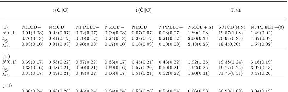
Table 1: Comparison of NCMD and NMCD+ methods. Values in the table are mean (stan-dard deviation in parentheses) for 100 replications.
points, ξ(C||Cˆ), and false positive changepoints, ξ( ˆC||C), i.e.,
ξ(C||Cˆ) = #C∈Cˆ
nC
and ξ( ˆC||C) = # ˆC∈/ C
nCˆ
, (4.1)
where ˆC are the estimated changepoints; C are the true changepoints; nCˆ is the length of
the estimated changepoint set and nC is the length of the true changepoint set. In addition
we also compare the computational time taken to run both of these methods. The results
can be seen in Table 1.
It is clear from Table 1 that using the screening step (NMCD+) significantly improves the
computational cost for this method. However using this screening step comes at a cost of not
correctly detecting the true changepoints. It can be seen that in all cases NMCD+ detects
fewer true positives and more false positives than NMCD.
We now turn to consider the choice of the screening windowNI further. Using Model 1 with
normal errors we can compare the results for different values ofNI. The default value for this
data is NI = 10, but we now repeat the analysis using NI ∈ {1, . . . ,12}. Figure 1a shows a
bar plot of the number of times (in 100 simulations) that the window size resulted in the same
changepoints as using NMCD without screening. Similarly Figure 1b looks at the number
of true and false positives found using the different window lengths in the screening step.
Figure 1c shows the computational time taken for NMCD+ with varying window lengthsNI.
100 99
97 97 96 96 96 96 96 96 96 96
0 25 50 75 100
1 2 3 4 5 6 7 8 9 10 11 12
Window size NI
Pr
opor
tion equal to NMCD
(a)
0.910 0.915 0.920 0.925
5 10
Window size NI
Pr
opor
tion of T
rue and F
asle c
hang
epoints
(b)
0 500 1000
5 10
Window size NI
Time
(c)
Figure 1: (a) The number of replications out of 100 in which using NMCD+ with varying NI
results in the same results as NMCD without screening. (b) The proportion of true (black) and 1-False (red) changepoints detected with varying window sizeNI. (c) The computational
time (secs) for NMCD+ with increasing window size NI.
It is clear that whilst in the majority of the cases NMCD+ with the different NI gives the
same result as NMCD but with an improved computational speed, there is a reasonable
proportion of data sets where NMCD+ does not find the optimal segmentation. As a result
the segmentations it obtains are less accurate.
The NMCD method also requires us to choose a penalty value in order to pick the best
segmentation. The default choice appears to work reasonably well, but resulted in slight
estimates of the number of changepoints for our three simulation scenarios. These
over-estimates suggest that the penalty value has been too small.
4.2
Comparison to NMCD
To compare NP-PELT to NMCD we initially used the same 3 models as above and again
looked at the accuracy of the methods and the computational time. As before, to implement
NMCD we used thenmcdr R package Zou and Zhange (2014) which has the bulk of the code
in FORTRAN and we used R code to run NP-PELT. As R code is slower than FORTRAN,
this means that the raw CPU timings we give will favour NMCD.
Firstly we investigate the speed up obtained by using the PELT pruning. We implement
PELT with the same segment costs as NMCD, and call this PELT. We found that
[image:12.612.85.527.72.235.2]0.00 0.25 0.50 0.75 1.00
10 20 30 40
Quantiles
Pr
opor
tion of T
rue and F
asle c
hang
epoints
(a)
0.00 0.05 0.10 0.15 0.20
10 20 30 40
Quantiles
Relative dif
erence in time
(b)
Figure 2: (a) The proportion of true positive changepoints for a range of quantiles, K, in NP-PELT+ (solid) in comparison to NP-PELT (dashed). Black: n = 500, red: n = 1000, blue: n = 2000 and grey: n = 5000. (b) Relative speed of using NP-PELT+ compared to using NP-PELT. with varying number of quantiles, K. Black: n = 500, red: n = 1000, blue:
n = 2000 and grey: n= 5000.
of magnitude slower than NMCD+.
4.3
Choice of
K
in NP-PELT
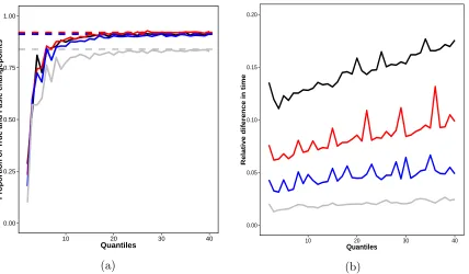
In order to use the improvement suggested in Section 3.1 for NP-PELT we first of all need
to decide on an appropriate value forK. We use Model 1 again to assess the performance of
NP-PELT using only K quantiles of the data (NP-PELT+), for a range of values of K, in
comparison to NP-PELT using the full data set. Here we only look at the model with normal
errors and simulate data-series with lengths n = (500,1000,2000,5000). Further simulations
using different error terms gave similar results. In order to assess performance we look at the
proportion of true positives detected using both methods and also the computational cost.
Again we use 100 replications. The results for the accuracy can be seen in Figure 2a.
We can see from Figure 2a that as the number of quantiles increases the proportion of true
[image:13.612.78.506.75.325.2]length of the data increases this convergence appears to happen more slowly, this can be
seen from the grey lines in Figure 2a, which represent data of length 5000. We suggest using
K = d4 log(n)e in order to conserve as much accuracy as possible. This choice corresponds
to K = 25, 28, 31 and 35 for n= 500, 1000, 2000 and 5000 respectively.
In addition to the accuracy we also look at the relative speed up of NP-PELT+ with various
K values in comparison to NP-PELT, i.e.,
(speed of NP-PELT+) speed of NP-PELT .
The results of this analysis can be seen in Figure 2b. Clearly as the number of quantiles
increases the relative speed up decreases. This is expected since the number of quantiles is
converging to the whole data set which is used in NP-PELT. We can also see that the relative
speed up of NP-PELT+ increases with increasing data length.
4.4
Comparison of NMCD and NP-PELT+
We next compare NP-PELT+ with K = 4 log(n) to NMCD as above. For this we perform
an equivalent analysis to that of Section 4.2. The results for NP-PELT+ can be found in
Table 1. In terms of accuracy we can see that NP-PELT+ is comparable to NMCD and
is significantly faster to run. In comparison to NMCD+, in Models 2 and 3 NP-PELT+ is
slightly slower. This is to be expected however as the results of Killick et al. (2012) imply
that the cost of PELT will tend to be lower in situations with more changepoints. In the
first model there are 11 changepoints in data sets of length 1000, however in Models 2 and
3 there are only 4 changepoints. Despite this method being slower than NMCD+ it is more
accurate.
5
Activity Tracking
In this section we apply NP-PELT+ to try to detect changes in heart rate during a run.
Wearable activity trackers are becoming increasingly popular devices used to record step
such as the Fitbit change HR (Fitbit Inc., San Francisco, CA), heart rate. The idea behind
these devices is that the ability to monitor your activity should help you lead a fit and active
lifestyle. Changepoint detection can be used in daily activity tracking data to segment the
day into periods of activity, rest and sleep.
Similarly, many keen athletes, both professional and amateur, also use GPS sports watches
which have the additional features of recording distance and speed which can be very
ben-eficial in training, especially in sports such as running and cycling. Heart rate monitoring
during training can help make sure you are training hard enough without over training and
burning out. Heart rate is the number of heart beats per unit time, normally we express this
as beats per minute (bpm).
5.1
Changepoints in heart rate data
In the changepoint and signal processing literature many authors have looked at heart rate
monitoring in different scenarios (see for example Khalfa et al. (2012); Galway et al. (2011);
Billat et al. (2009); Staudacher et al. (2005)). Aubert et al. (2003) give a detailed review of
the influence of heart rate variability in athletes. They highlight the difficulty of analysing
heart rate measurements during exercise since no steady state is obtained due to the heart
rate variability increasing according to the intensity of the exercise. They note that one
possible solution is to pre-process the data to remove the trend.
In this section we apply NP-PELT+ to see whether changes can be detected in the raw heart
rate time series without having to initially pre-process the data. We use a nonparametric
approach since heart rate is a stochastic time dependent series and thus does not satisfy
the conditions for an IID Normal model. However we will compare the performance had we
assumed that the data was Normal in Section 5.3. The aim is to develop a method which can
be used on data recorded from commercially available devices without the need to pre-process
5.2
Range of Penalties
One disadvantage of NP-PELT+ over NMCD is that NP-PELT+ produces a single
segmen-tation, which is optimal for the pre-chosen penalty value ξn. By comparison, NCMD finds
a range of segmentations, one for each of m = 1, . . . , M changepoints (though, in practice,
the nmcdr package only outputs a single segmentation). Whilst there are default choices
for ξn, these do not always work well, and there are advantages to being able to compare
segmentations with different number of changepoints.
Haynes et al. (2015) propose a method, Changepoints over a Range Of PenaltieS (CROPS),
which efficiently finds all the optimal segmentations for penalty values across a continuous
range. This involves an iterative procedure which chooses values of ξn to run NP-PELT on,
based on the segmentations obtained from previous runs of NP-PELT for different penalty
values. Assume we have a given range [ξmin, ξmax] for the penalty value, and the optimal
seg-mentations at ξmin and ξmax have mmin and mmax changepoints respectively. Then CROPS
requires at most mmin−mmax+ 2 runs of NP-PELT to be guaranteed to find all optimal
seg-mentations forξn∈[ξmin, ξmax]. Furthermore, it is possible to recycle many of the calculations
from early runs of NP-PELT to speed up the later runs.
5.2.1 Nonparametric Changepoint Detection
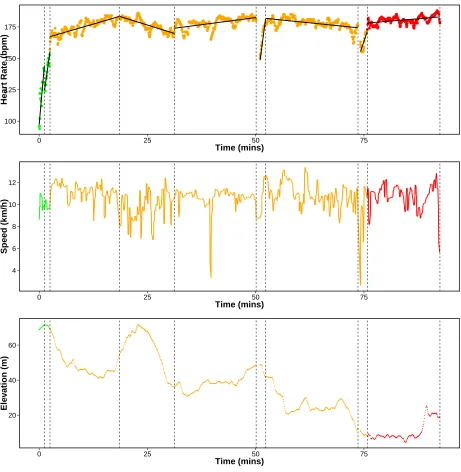
An example data set is given in Figure 4, where we show heart-rate, speed and elevation
recorded during a 10 mile run. We will aim to segment this data using the heart-rate data
only, but include the other two series in order that we may assess how well the segmentation
of the heart-rate data relates to the obvious different phases of the run. In training many
people use heart rate as an indicator of how hard they are working. There are different
heart rate zones that you can train in each of which enhances different aspects of your fitness
(BrainMacSportsCoach, 2015). The training zones are defined in terms of percentages of a
maximum heart-rate: peak (90-100%), anaerobic (80-90%), aerobic (70-80%) and recovery
(<70%).
This example looks at detecting changes in heart rate over a long undulating run. We
use CROPS with NP-PELT+ with ξmin = 25, ξmax = 200 and K = 4 log(n) (the results
(a) Elbow plot for NP-PELT+
● ● ● ● ● ● ● ● ● ● ● ● ● ● ● ●
● ● ● ● ● ● ● ● ● ● ● ● ● ● ● ●
1500 2000 2500 3000
10 20
Number of Changepoints
Cost
(b) Elbow plot for a change in slope
● ● ● ● ● ● ● ● ● ● ● ● ● ● ● ● ● ● ●
● ● ● ● ● ● ● ● ● ● ● ● ● ● ● ● ● ● ●
10000 20000 30000
5 10 15 20 25
Number of Changepoints
[image:17.612.161.453.74.250.2]Cost
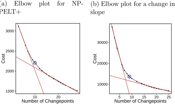
Figure 3: The cost vs number of changepoints plotted for (a) NP-PELT+ and (b) Change in slope. the red lines indicate the elbow and the blue circle highlights the point that we use as being the centre of the elbow.
suggested by Lavielle (2005). This involves plotting the segmentation cost against the number
of changepoints and then looking for an “elbow” in the plot. The points on the “elbow” are
then suggested to be the most feasible segmentations. The intuition for this method is
that as more true changepoints are detected the cost will decrease however as we detect
more changepoints we are likely to be detecting false positives and as such the cost will not
decrease as much. The plot of the “elbow” for this example can be seen in Figure 3a. The
elbow is not always obvious therefore the choice can be subjective however this gives us a
method for roughly choosing the best segmentations which we can then explore further. We
have highlighted the points on the “elbow” as the points which are between the two red lines.
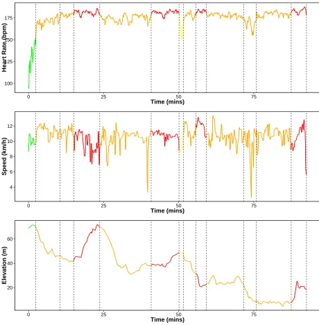
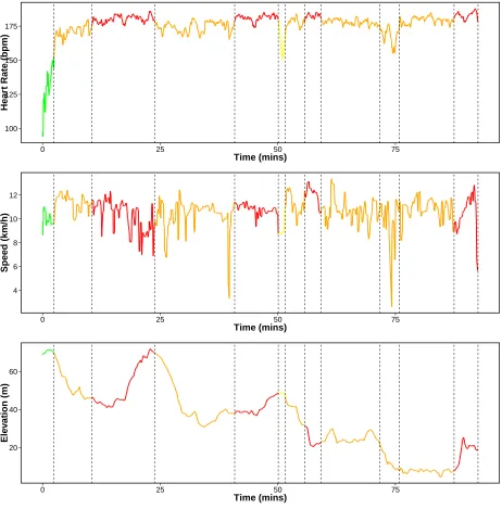
We decided from this plot that the segmentations with 9, 10, 12 and 13 changepoints are the
best. We illustrate the segmentation with 10 changepoints, the number of changepoints at
the centre of the elbow in Figure 3a indicated by the blue circle, in Figure 4. The segments
have been colour coded based on the average heart-rate in each segment. That is red: peak,
orange: anaerobic, yellow: aerobic and green: recovery. Alternative segmentations from the
number of changepoints on the elbow can be found in the supplementary material.
We superimpose the changepoints detected in the heart rate onto the plots for speed and
elevation to see if we can explain any of the changepoints. The first segment captures the
100 125 150 175
4 6 8 10 12
20 40 60
0 25 50 75
0 25 50 75
0 25 50 75
Time (mins)
Time (mins)
Time (mins)
Hear
t Rate (bpm)
Speed (km/h)
Ele
v
[image:18.612.75.537.135.605.2]ation (m)
anaerobic zone. The heart-rate in the second segment is in the anaerobic zone but changes
to the peak zone in segment three. This change initially corresponds to an increase in speed
and then it is because of the steep incline. The third changepoint matches up to the top of
the elevation which is the start of the fourth segment where the heart-rate drops into the
anaerobic zone whilst running downhill. The fifth segment is red which might be as a result
of both the speed being slightly higher than the previous segment and consistent, and a slight
incline in elevation. This is followed by a brief time in the aerobic zone which could be due
to a drop in speed. The heart-rate in the next three segments stays in the anaerobic zone.
The changepoints that split this section into three segments relate to the dip in speed around
75 minutes. In the final segment the heart-rate is in the peak zone which corresponds to an
increase in elevation and an increase in speed (a sprint finish).
5.3
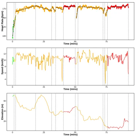
Piece-wise linear model
For comparison we look at estimating the changepoints based on a penalised likelihood
ap-proach that assumes the data is normally distributed with a mean that is piecewise linear
within each segment. To find the best segmentation we use PELT with a segment cost
proportional to minus the log-likelihood of our model:
C(ys:t) = minθ1,θ2
t
X
u=s
(yu−θ1 −uθ2)2, (5.1)
where θ1 and θ2 and the estimates of the segment intercept and slope, respectively. We use
CROPS to find the best segmentation under this criteria for a range of penalties. The
re-sulting elbow plot can be seen in Figure 3b. We can see that the number of changepoints for
the feasible segmentations is similar to the number of changepoints for using NP-PELT+.
Figure 5 shows the segmentation with 9 changepoints which we have deduced to being the
number of changepoints in the centre of the elbow in Figure 3b. Alternative segmentations
from the number of changepoints on the elbow can be found in the supplementary material.
It is obvious from the first look at Figure 5 that the change in slope method has not detected
of the plot is coloured orange with only changes in the first and last segments. The change
in slope method splits the “warm-up” period into two segments whereas having this as one
segment appears more appropriate. Unlike NP-PELT+ the change in slope does not detect
changes which correspond to the change in elevation and thus NP-PELT+ appears to split
the heart-rate data into more appropriate segments which relate to different phases of the
run.
6
Conclusion
We have developed a new algorithm, NP-PELT, to detect changes in data series where we
do not know the underlying distribution. This method is an adaption of the NMCD method
proposed by Zou et al. (2014). The main advantage of NP-PELT over NMCD is that it is
orders of magnitude faster. We initially reduced the time to calculate the cost of a segment
fromO(n) toO(logn) by simplifying the definition of the segment cost. Zou et al. (2014) use
a screening step to improve the computational time and even though this is slightly faster
than NP-PELT we show that it isn’t as accurate. We have also shown that non-parametric
changepoint detection, using NP-PELT, holds promise for segmenting data from activity
trackers. We were able to segment heart-rate data recorded during a run into meaningful
segments that correspond to different phases of the run, and can be related to different
regimes of heart-rate activity.
Acknowledgements Haynes gratefully acknowledges the support of the EPSRC funded
EP/H023151/1 STOR-i centre for doctoral training and the Defence Science and Technology
Laboratory.
References
Aubert, A. E., Seps, B., and Beckers, F. (2003). Heart rate variability in athletes. Sports Medicine, 33(12):889–919.
● ● ● ● ● ● ● ● ● ● ●● ● ● ● ●●● ● ● ●● ● ● ● ●●● ● ●●● ● ● ● ●● ● ● ● ● ● ● ● ● ● ● ●●● ● ● ●●● ●●● ● ● ●●●●●● ● ●● ● ● ●●●●●●●● ● ● ● ●●●●●●●●●●●●●●●● ● ●●●●● ● ●●●●●●●●●● ● ●●●●● ● ●●●●●● ●●●●● ● ● ● ●●● ●●●●● ●●●●●●●●●●●●●●●● ●●●●●●●●● ●●●●●●●●●●●●●●●●●●●●●●●●●●●●●●●●●●● ●●●●●●●●● ● ●●●●●●●● ●●● ●●● ●●● ●●●●●●●●●●●●●●●●●●●●●●●●●●● ● ●●●●●●●●●●●●●●●●●●●●●●●●●●● ●●●●●● ● ● ● ●●●●●●●●●● ● ●●●●●●●●●●●●●●●●●●●●●●●● ●● ●●●●●●●●●●●●●●● ●●● ● ● ●●● ● ●●●●●●●●●●●●●●●●●●●●●●●●● ●●●●●●●●●●●●●●●●●●●●●●●●●●●●●●● ●●●●●● ●●● ● ● ●●● ●●●● ● ●● ● ●● ● ●●●●●●●●●●●● ●●● ●●●●●●●●●●●●●● ● ●●●●●●●●●●●●●●●●●●●●● ●●●●●●●●●●●●●●●● ●●●●●● ●●●●● ● ●●● ● ● ● ●●●●●●●●●● ● ●●● ● ●●●●●●●●● ●●●●● ● ●●●●●●●●●●●● ●●●●● ●●● ●● ●●●●●●●● ● ● ●●●●●●● ● ●●●●●●●●●●●●●●●●●●●●●● ● ●●●●●●●●●●● ● ●●●●●●●●● ● ●●●●●● ●●●● ● ●● ● ●●●●●●●●●●● ●●●●●●●●●●●●● ●●● ● ●● ●● ● ●●●●●●●●● ●●● ●●●●●●●●● ● ●●●●●●●●●●●●●●●●●●●●●●●●●●●●●●●● ● ●●● ●●●●●●●●●●●●●●●●●●●●●●●●●●●●●●●●●●●●●●●●●●●●●●●●●●●● ● ●● ●●●●● ● ●●●●●●●●●●●●●●●● ● ●●●●●●●●●●●● ●●●●●●●●●● ● ● ● ●●●●●●●●●●●●●●●●●●●●●●●●● ● ●●●●● ● ●●●●●●●●●●●●●●● ●●●●●●●● ●●● ● ● ●●● ● ●● ● ●●● ● ● ● ●●●●● ● ● ●●● ● ● ● ● ● ●●● ●●●● ● ●●●●●●● ● ● ●● ●● ●● ●●●● ● ●●●●●●●●●●●●● ● ● ● ●●●●●●●●●●●●●●●●●●●●●●●●●●●●●●●●●●● ● ●●●●●●●●●●●●●●●●●●●● ● ●●●●● ● ●●●●● ● ●●●●●●●●●●● ● ●●● ●●●●●●●●●●●●●●●●●●● ●●●●● ● ●●●●●●●●●●●● ● ●●●●●●●●●● ● ●●●●●●●●●● ●●●●●●●●●●●●●●●●●●●●●●●●●●●●●●●●●●●●● ● ● ● ●●●●●●●●●●●●●●●●●●●●●●●●●●●●●●●●●●●●●●●●● ● ● ●●●● ● ● ●● ● ● ● ● ● ● ● ● ● ● ● ● ●●●●●●●●●●● ● ● ●● ● ● ●● ● ●● ● ●●●● ●● ● ●● ●●● ●●●●●●●●●●●●●●● ● ● ●●●●●●● ●●●●●●●●●●●●●●●●●●●●●●●●●●●● ●●●●●●●●●●●●●●●●●●●●●●●●●●●● ● ●●●●●●●●●●●●●●●●●●●●●●●●●● ●●●●●●●●●●●●●●●●●●●●●●●●● ● ●● ● ● ●●●●● ●●●●●●●●●●●●● ● ● ●●●●●●●●●●●●●●●●●● ● ● ●●●●●●●● ●●●●●●●●●●●●● ●●●●●●●●●●●●●● ●●●●●●●●●●●●●●●●●●●●●●●●●●●●●●●●●●●●●●●● ●●● ● ●●●● ● ●●●●●● ● ● ● ● ● ● ●● ●● ●● ●●●●● ● ● ● ● ●● ● ●● ● ● ● ● ● ●● ● ● ●● ● ●● ●● ● ● ● ● ●●●●●●●●●●●●● ● ●●●●●●●● ●●●●● ●●●●●● ●● ● ● ● ● ● ●●●●●●●●●●●●●●●●● ●●●●●●●●●●●●●●●●●●●●●●● ●●●●● ●●●●●●●● ●●●●●●●●●●● ●● ●●●●●●●●●●●●●●●●●●●●●●●●●●●●●●●●●●●●●●●●●●●●●●●●●●● ●●● ●● ● ●●●●●●●●●●●●●●●● ●●●●●●●●●●●●●●● ●●●● ●●●●●● ●●●●●●●●●●●●●●●●●●●●●●●●●●●●●●●● ● ● ● ● ● ●●●●●●●●●●●●●●● ●●●●●●●●● ● ● ● ● ● ● ● ● ●●● ●●●●●●●●●●●●●●●●●●● ● ● ● ● ● ● ● ●●●●●●●●●●● ●●●●●●●●●●●●●●●●●●●●●●●●●● ●● ●●●●●●●●●●●●●●●●●●●●●●● ● ● ● ● ●● ● ● ● ● ●●●●●●●●●●●●●●●●●●●●●●● ●●●●●●●●●●●●●●●●●●●●●●●●●●●●●●●●●●●●●●●●●●●●●●●●●●●●●●●●●●●●●●●●●●●●●● ● ●●● ● ● ●● ●● ●●●●●●● ● ●● ● ● ●● ●● ●●●●●●● ● ● ● ● ● ● ●●●●●● ●●●●●● ●●●●●●●●●●●●●●●●●● ●●●● ●●● ●● ●●●●●●●●●●●●●● ●●●●●●●●●●●●●●●● ●●●●●●●●●●●●●●●●●●●●●●●●●●●●●●●●●●●●●●●●●●●●●●●●●●●●●●●●●●●●●●●● ● ●●●●●●●●●●●●●●●●●●●●●●●●●●●●●●●●● ●●●●●●●●●●●●●●●●●●●● ●●●●●●● ● ● ● ● ● ● ● ● ●● ● ● ● ● ● ●● ●●● ●●●●●●●●●●●●●●●●●●●●●● ●●●●●●● 100 125 150 175 4 6 8 10 12 20 40 60
0 25 50 75
0 25 50 75
0 25 50 75
Time (mins)
Time (mins)
Time (mins)
Hear
t Rate (bpm)
Speed (km/h)
Ele
v
[image:21.612.75.536.125.597.2]ation (m)
Auger, I. and Lawrence, C. (1989). Algorithms for the Optimal Identification of Segment
Neighborhoods. Bulletin of Mathematical Biology, 51(1):39–54.
Bai, J. and Perron, P. (1998). Estimating and testing linear models with multiple structural
changes. Econometrica, 66:47–78.
Baron, M. (2000). Nonparametric adaptive change-point estimation and on-line detection.
Sequential Analysis, 19:1–23.
Bhattacharyya, G. and Johnson, R. (1968). Nonparametric tests for shift at an unknown
time point. The Annals of Mathematical Statistics, 39(5):1731–1743.
Billat, V. L., Mille-Hamard, L., Meyer, Y., and Wesfreid, E. (2009). Detection of changes
in the fractal scaling of heart rate and speed in a marathon race. Physica A: Statistical Mechanics and its Applications, 388(18):3798 – 3808.
BrainMacSportsCoach (2015). Heart rate training zones. https://http://www.brianmac.
co.uk/hrm1.htm.
Carlstein, E. (1988). Nonparametric change-point estimation. The Annals of Statistics, 16(1):188–197.
Davis, R. A., Lee, T. C. M., and Rodriguez-Yam, G. A. (2006). Structural Break Estimation
for Nonstationary Time Series Models. Journal of the American Statistical Association, 101(473):223–239.
Dette, H. and Wied, D. (2015). Detecting relevant changes in time series models. Journal of the Royal Statistical Society: Series B (Statistical Methodology).
Dumbgen, L. (1991). The asymptotic behavior of some nonparametric change-point
estima-tors. The Annals of Statistics, 19(3):1471–1495.
Frick, K., Munk, A., and Sieling, H. (2014). Multiscale change point inference. Journal of the Royal Statistical Society: Series B (Statistical Methodology), 76(3):495–580.
Galway, L., Zhang, S., Nugent, C., McClean, S., Finlay, D., and Scotney, B. (2011).
Uti-lizing wearable sensors to investigate the impact of everyday activities on heart rate. In
Abdulrazak, B., Giroux, S., Bouchard, B., Pigot, H., and Mokhtari, M., editors, Toward Useful Services for Elderly and People with Disabilities, volume 6719 of Lecture Notes in Computer Science, pages 184–191. Springer Berlin Heidelberg.
Guarnaccia, C., Quartieri, J., Tepedino, C., and Rodrigues, E. R. (2015). An analysis of
airport noise data using a non-homogeneous Poisson model with a change-point. Applied Acoustics, 91:33–39.
Haynes, K., Eckley, I. A., and Fearnhead, P. (2015). Computationally efficient changepoint
detection for a range of penalties. Journal of Computational and Graphical Statistics (to appear).
Jackson, B., Scargle, J. D., Barnes, D., Arabhi, S., Alt, A., Gioumousis, P., Gwin, E.,
Sang-trakulcharoen, P., Tan, L., and Tsai, T. T. (2005). An algorithm for optimal partitioning
of data on an interval. Signal Processing, pages 1–4.
Jandhyala, V., Fotopoulos, S., MacNeill, I., and Liu, P. (2013). Inference for single and
multiple change-points in time series. Journal of Time Series Analysis, 34(4):423–446. Khalfa, N., Bertandm, P. R., Boudet, G., Chamoux, A., and Billat, V. (2012). Heart rate
regulation processed through wavelet analysis and change detection: some case studies.
Acta Biotheoretica, 60:109 – 29.
Killick, R., Fearnhead, P., and Eckley, I. A. (2012). Optimal detection of changepoints with a
linear computational cost. Journal of the American Statistical Association, 107(500):1590– 1598.
Lavielle, M. (2005). Using penalized contrasts for the change-point problem. Signal Process-ing, 85(8):1501–1510.
Lu, L. and Zhang, H.-j. (2002). Speaker Change Detection and Tracking in Real-Time
News Broadcasting Analysis. Proceedings of the tenth ACM international conference on multimedia, pages 602–610.
Matteson, D. S. and James, N. A. (2013). A Nonparametric Approach for Multiple Change
Point Analysis of Multivariate Data. 14853:1–29.
Nam, C. F. H., Aston, J. A. D., Eckley, I. A., and Killick, R. (2014). The Uncertainty
of Storm Season Changes: Quantifying the Uncertainty of Autocovariance Changepoints.
Technometrics, (January 2015):00–00.
Olshen, A. B., Venkatraman, E. S., Lucito, R., and Wigler, M. (2004). Circular binary
segmentation for the analysis of array-based DNA copy number data.Biostatistics (Oxford, England), 5(4):557–72.
Page, E. (1954). Continuous inspection schemes. Biometrika, 41(1):100–115.
Pettitt, A. (1979). A non-parametric approach to the change-point problem. Applied statis-tics, 28(2):126–135.
Ross, G. and Adams, N. M. (2012). Two Nonparametric Control Charts for Detecting
Arbitrary Distribution Changes. Journal of Quality Technology, 44(2):102–116.
Schwarz, G. (1978). Estimating the Dimension of a Model.The Annals of Statistics, 6(2):461– 464.
Scott, A. and Knott, M. (1974). A cluster analysis method for grouping means in the analysis
of variance. Biometrics, 30:507–512.
Staudacher, M., Telser, S., Amann, A., Hinterhuber, H., and Ritsch-Marte, M. (2005). A
new method for change-point detection developed for on-line analysis of the heart beat
variability during sleep. Physica A: Statistical Mechanics and its Applications, 349(3):582– 96.
Zhang, J. (2002). Powerful goodness-of-fit tests based on the likelihood ratio. Journal of the Royal Statistical Society Series B, 64(2):281–294.
Zhang, N. R. and Siegmund, D. O. (2007). A modified Bayes information criterion with
appli-cations to the analysis of comparative genomic hybridization data.Biometrics, 63(1):22–32. Zou, C., Yin, G., Feng, L., and Wang, Z. (2014). Nonparametric maximum likelihood
ap-proach to multiple change-point problems. The Annals of Statistics, 42(3):970–1002. Zou, C. and Zhange, L. (2014). nmcdr: Non-parametric Multiple Change-Points Detection.
SUPPLEMENTARY MATERIAL
Further Results - NP-PELT+
100 125 150 175
4 6 8 10 12
20 40 60
0 25 50 75
0 25 50 75
0 25 50 75
Time (mins)
Time (mins)
Time (mins)
Hear
t Rate (bpm)
Speed (km/h)
Ele
v
[image:26.612.73.533.148.616.2]ation (m)
Figure 1: Segmentations using NP-PELT+ with 13 changepoints. We have colour coded the line based on the average heart-rate of each segment where red: peak, orange: anaerobic, yellow: aerobic and green: recovery.
100 125 150 175
4 6 8 10 12
20 40 60
0 25 50 75
0 25 50 75
0 25 50 75
Time (mins)
Time (mins)
Time (mins)
Hear
t Rate (bpm)
Speed (km/h)
Ele
v
[image:27.612.75.537.135.604.2]ation (m)
100 125 150 175
4 6 8 10 12
20 40 60
0 25 50 75
0 25 50 75
0 25 50 75
Time (mins)
Time (mins)
Time (mins)
Hear
t Rate (bpm)
Speed (km/h)
Ele
v
[image:28.612.75.537.135.604.2]ation (m)
Further Results - Piece-wise linear ● ● ● ● ● ● ● ● ● ● ●● ● ● ● ●●● ● ● ●● ● ● ● ●●● ● ●●● ● ● ● ●● ● ● ● ● ● ● ● ● ● ● ●●● ● ● ● ●●●●● ● ● ●●●●●● ● ●● ● ● ●●●●●●●● ● ● ● ●●●●●●●●●●●●●●●● ● ●●●●● ● ●●●●●●●●●● ● ●●●●● ● ●●●●●● ●●●●● ● ● ● ●●● ●●●●● ●●●●●●●●●●●●● ● ● ●●●●●●●●●● ●●●●●●●●●●●●●●●●●●●●●●●●●●●●●●●●●●● ●●●●●●●●● ● ●●●●●●●● ●● ● ●●●●●● ●●●●●●●●●●●●●●●●●●●●●●●●●●● ● ●●●●●●●●●●●●●●●●●●●●●●●●●●● ●●●●●● ● ● ● ●●●●●●●●●● ● ●●●●●●●●●●●●●●●●●●●●●●●●●● ●●●●●●●●●●●●●●● ●● ●●●●●● ● ●●●●●●●●●●●●●●●●●●●●●●●●●●●●●●●●●●●●●●●●●●●●●●●●●●●●●● ● ●●●●●●● ●●● ● ● ●●●●●●●● ●● ● ●● ● ●●●●●●●●●●●● ●●● ●●●●●●●●●●●●●● ● ●●●●●●●●●●● ●●●●●● ● ●●●●●●●●●●●●●●●●●● ●●●●●●● ●●●●● ● ●●● ● ● ● ●●●●●●●●●● ● ●●● ● ●●●●●●●●● ●●●●● ● ●●●●●●●●●●●● ●●●●● ●●● ●●●●●●●●●● ● ● ●●●●●●● ● ●●●●●●●●●●●●●●●●●●●●●● ● ●●●●●●●●●●● ● ●●●●●●●●● ● ●●●●●● ●●●● ● ●● ● ●●●●●●●●●●● ●●●●●●●●●● ●●● ●●● ● ●● ●● ● ●●●●●●●●● ●● ● ●●●●●●●●● ● ●●●●●●●●●●●●●●●●●●●●●●●●●●●●●●●● ● ●●● ●●●●●●●●●●●●●●●●●●●●●●●●●●●●●●●●●●●●●●●●●●●●●●●●●●●● ● ●● ●●●●● ● ●●●●●●●●●●●●●●●● ● ●●●●●●●●●●●● ●●●●●●●●● ● ●●●●●●●●●●●●●●●●●●●●●●● ●●●●● ● ●●●●● ● ●●●●●●●●●●●●●●●●●●●●●●● ●●● ● ● ●●● ● ●● ● ●●● ● ● ● ●●●●● ● ● ●●● ● ● ● ● ● ●●● ●●●● ● ●●●●●●● ● ● ●● ● ● ●● ●●●● ● ●●●●●●●●●●●●●●● ● ●●●●●●●●●●●●●●●●●●●●●●●●●●●●●●●●●●● ● ●●●●●●●●●●●●●●●●●●●● ● ●●●●● ● ●●●●● ● ●●●●●●●●●●● ● ●●● ●●●●●●●●●●●● ●●●●●● ● ●●●●● ● ●●●●●●●●●●●● ● ●●●●●●●●●●● ●●●●●●●●●● ●●●●●●●●●●●●●●●●●●●●●●●●●●●●●●●●●●●●● ● ● ● 100 125 150 175 4 6 8 10 12 20 40 60
0 25 50 75
0 25 50 75
0 25 50 75
Time (mins)
Time (mins)
Time (mins)
Hear
t Rate (bpm)
Speed (km/h)
Ele
v
[image:29.612.71.541.112.585.2]ation (m)
● ● ● ● ● ● ● ● ● ● ●● ● ● ● ●●● ● ● ●● ● ● ● ●●● ● ●●● ● ● ● ●● ● ● ● ● ● ● ● ● ● ● ●●● ● ● ●●● ●●● ● ● ●●●●●● ● ●● ● ● ●●●●●●●● ● ● ● ●●●●●●●●●●●●●●●● ● ●●●●● ● ●●●●●●●●●● ● ●●●●● ● ●●●●●● ●●●●● ● ● ● ●●● ●●●●● ●●●●●●●●●●●●●●●● ●●●●●●●●● ●●●●●●●●●●●●●●●●●●●●●●●●●●●●●●●●●●● ●●●●●●●●● ● ●●●●●●●● ●●● ●●● ●●● ●●●●●●●●●●●●●●●●●●●●●●●●●●● ● ●●●●●●●●●●●●●●●●●●●●●●●●●●● ●●●●●● ● ● ● ●●●●●●●●●● ● ●●●●●●●●●●●●●●●●●●●●●●●● ●● ●●●●●●●●●●●●●●● ●●● ● ● ●●● ● ●●●●●●●●●●●●●●●●●●●●●●●●● ●●●●●●●●●●●●●●●●●●●●●●●●●●●●●●● ●●●●●● ●●● ● ● ●●● ●●●● ● ●● ● ●● ● ●●●●●●●●●●●● ●●● ●●●●●●●●●●●●●● ● ●●●●●●●●●●●●●●●●●●●●● ●●●●●●●●●●●●●●●● ●●●●●● ●●●●● ● ●●● ● ● ● ●●●●●●●●●● ● ●●● ● ●●●●●●●●● ●●●●● ● ●●●●●●●●●●●● ●●●●● ●●● ●● ●●●●●●●● ● ● ●●●●●●● ● ●●●●●●●●●●●●●●●●●●●●●● ● ●●●●●●●●●●● ● ●●●●●●●●● ● ●●●●●● ●●●● ● ●● ● ●●●●●●●●●●● ●●●●●●●●●●●●● ●●● ● ●● ●● ● ●●●●●●●●● ●●● ●●●●●●●●● ● ●●●●●●●●●●●●●●●●●●●●●●●●●●●●●●●● ● ●●● ●●●●●●●●●●●●●●●●●●●●●●●●●●●●●●●●●●●●●●●●●●●●●●●●●●●● ● ●● ●●●●● ● ●●●●●●●●●●●●●●●● ● ●●●●●●●●●●●● ●●●●●●●●●● ● ● ● ●●●●●●●●●●●●●●●●●●●●●●●●● ● ●●●●● ● ●●●●●●●●●●●●●●● ●●●●●●●● ●●● ● ● ●●● ● ●● ● ●●● ● ● ● ●●●●● ● ● ●●● ● ● ● ● ● ●●● ●●●● ● ●●●●●●● ● ● ●● ●● ●● ●●●● ● ●●●●●●●●●●●●● ● ● ● ●●●●●●●●●●●●●●●●●●●●●●●●●●●●●●●●●●● ● ●●●●●●●●●●●●●●●●●●●● ● ●●●●● ● ●●●●● ● ●●●●●●●●●●● ● ●●● ●●●●●●●●●●●●●●●●●●● ●●●●● ● ●●●●●●●●●●●● ● ●●●●●●●●●● ● ●●●●●●●●●● ●●●●●●●●●●●●●●●●●●●●●●●●●●●●●●●●●●●●● ● ● ● 100 125 150 175 4 6 8 10 12 20 40 60
0 25 50 75
0 25 50 75
0 25 50 75
Time (mins)
Time (mins)
Time (mins)
Hear
t Rate (bpm)
Speed (km/h)
Ele
v
[image:30.612.73.539.125.595.2]ation (m)
● ● ● ● ● ● ● ● ● ● ●● ● ● ● ●●● ● ● ●● ● ● ● ●●● ● ●●● ● ● ● ●● ● ● ● ● ● ● ● ● ● ● ●●● ● ● ●●● ●●● ● ● ●●●●●● ● ●● ● ● ●●●●●●●● ● ● ● ●●●●●●●●●●●●●●●● ● ●●●●● ● ●●●●●●●●●● ● ●●●●● ● ●●●●●● ●●●●● ● ● ● ●●● ●●●●● ●●●●●●●●●●●●●●●● ●●●●●●●●● ●●●●●●●●●●●●●●●●●●●●●●●●●●●●●●●●●●● ●●●●●●●●● ● ●●●●●●●● ●●● ●●● ●●● ●●●●●●●●●●●●●●●●●●●●●●●●●●● ● ●●●●●●●●●●●●●●●●●●●●●●●●●●● ●●●●●● ● ● ● ●●●●●●●●●● ● ●●●●●●●●●●●●●●●●●●●●●●●● ●● ●●●●●●●●●●●●●●● ●●● ● ● ●●● ● ●●●●●●●●●●●●●●●●●●●●●●●●● ●●●●●●●●●●●●●●●●●●●●●●●●●●●●●●● ●●●●●● ●●● ● ● ●●● ●●●● ● ●● ● ●● ● ●●●●●●●●●●●● ●●● ●●●●●●●●●●●●●● ● ●●●●●●●●●●●●●●●●●●●●● ●●●●●●●●●●●●●●●● ●●●●●● ●●●●● ● ●●● ● ● ● ●●●●●●●●●● ● ●●● ● ●●●●●●●●● ●●●●● ● ●●●●●●●●●●●● ●●●●● ●●● ●● ●●●●●●●● ● ● ●●●●●●● ● ●●●●●●●●●●●●●●●●●●●●●● ● ●●●●●●●●●●● ● ●●●●●●●●● ● ●●●●●● ●●●● ● ●● ● ●●●●●●●●●●● ●●●●●●●●●●●●● ●●● ● ●● ●● ● ●●●●●●●●● ●●● ●●●●●●●●● ● ●●●●●●●●●●●●●●●●●●●●●●●●●●●●●●●● ● ●●● ●●●●●●●●●●●●●●●●●●●●●●●●●●●●●●●●●●●●●●●●●●●●●●●●●●●● ● ●● ●●●●● ● ●●●●●●●●●●●●●●●● ● ●●●●●●●●●●●● ●●●●●●●●●● ● ● ● ●●●●●●●●●●●●●●●●●●●●●●●●● ● ●●●●● ● ●●●●●●●●●●●●●●● ●●●●●●●● ●●● ● ● ●●● ● ●● ● ●●● ● ● ● ●●●●● ● ● ●●● ● ● ● ● ● ●●● ●●●● ● ●●●●●●● ● ● ●● ●● ●● ●●●● ● ●●●●●●●●●●●●● ● ● ● ●●●●●●●●●●●●●●●●●●●●●●●●●●●●●●●●●●● ● ●●●●●●●●●●●●●●●●●●●● ● ●●●●● ● ●●●●● ● ●●●●●●●●●●● ● ●●● ●●●●●●●●●●●●●●●●●●● ●●●●● ● ●●●●●●●●●●●● ● ●●●●●●●●●● ● ●●●●●●●●●● ●●●●●●●●●●●●●●●●●●●●●●●●●●●●●●●●●●●●● ● ● ● 100 125 150 175 4 6 8 10 12 20 40 60
0 25 50 75
0 25 50 75
0 25 50 75
Time (mins)
Time (mins)
Time (mins)
Hear
t Rate (bpm)
Speed (km/h)
Ele
v
[image:31.612.74.535.127.595.2]ation (m)
● ● ● ● ● ● ● ● ● ● ●● ● ● ● ●●● ● ● ●● ● ● ● ●●● ● ●●● ● ● ● ●● ● ● ● ● ● ● ● ● ● ● ●●● ● ● ●●● ●●● ● ● ●●●●●● ● ●● ● ● ●●●●●●●● ● ● ● ●●●●●●●●●●●●●●●● ● ●●●●● ● ●●●●●●●●●● ● ●●●●● ● ●●●●●● ●●●●● ● ● ● ●●● ●●●●● ●●●●●●●●●●●●●●●● ●●●●●●●●● ●●●●●●●●●●●●●●●●●●●●●●●●●●●●●●●●●●● ●●●●●●●●● ● ●●●●●●●● ●●● ●●● ●●● ●●●●●●●●●●●●●●●●●●●●●●●●●●● ● ●●●●●●●●●●●●●●●●●●●●●●●●●●● ●●●●●● ● ● ● ●●●●●●●●●● ● ●●●●●●●●●●●●●●●●●●●●●●●● ●● ●●●●●●●●●●●●●●● ●●● ● ● ●●● ● ●●●●●●●●●●●●●●●●●●●●●●●●● ●●●●●●●●●●●●●●●●●●●●●●●●●●●●●●● ●●●●●● ●●● ● ● ●●● ●●●● ● ●● ● ●● ● ●●●●●●●●●●●● ●●● ●●●●●●●●●●●●●● ● ●●●●●●●●●●●●●●●●●●●●● ●●●●●●●●●●●●●●●● ●●●●●● ●●●●● ● ●●● ● ● ● ●●●●●●●●●● ● ●●● ● ●●●●●●●●● ●●●●● ● ●●●●●●●●●●●● ●●●●● ●●● ●● ●●●●●●●● ● ● ●●●●●●● ● ●●●●●●●●●●●●●●●●●●●●●● ● ●●●●●●●●●●● ● ●●●●●●●●● ● ●●●●●● ●●●● ● ●● ● ●●●●●●●●●●● ●●●●●●●●●●●●● ●●● ● ●● ●● ● ●●●●●●●●● ●●● ●●●●●●●●● ● ●●●●●●●●●●●●●●●●●●●●●●●●●●●●●●●● ● ●●● ●●●●●●●●●●●●●●●●●●●●●●●●●●●●●●●●●●●●●●●●●●●●●●●●●●●● ● ●● ●●●●● ● ●●●●●●●●●●●●●●●● ● ●●●●●●●●●●●● ●●●●●●●●●● ● ● ● ●●●●●●●●●●●●●●●●●●●●●●●●● ● ●●●●● ● ●●●●●●●●●●●●●●● ●●●●●●●● ●●● ● ● ●●● ● ●● ● ●●● ● ● ● ●●●●● ● ● ●●● ● ● ● ● ● ●●● ●●●● ● ●●●●●●● ● ● ●● ●● ●● ●●●● ● ●●●●●●●●●●●●● ● ● ● ●●●●●●●●●●●●●●●●●●●●●●●●●●●●●●●●●●● ● ●●●●●●●●●●●●●●●●●●●● ● ●●●●● ● ●●●●● ● ●●●●●●●●●●● ● ●●● ●●●●●●●●●●●●●●●●●●● ●●●●● ● ●●●●●●●●●●●● ● ●●●●●●●●●● ● ●●●●●●●●●● ●●●●●●●●●●●●●●●●●●●●●●●●●●●●●●●●●●●●● ● ● ● 100 125 150 175 4 6 8 10 12 20 40 60
0 25 50 75
0 25 50 75
0 25 50 75
Time (mins)
Time (mins)
Time (mins)
Hear
t Rate (bpm)
Speed (km/h)
Ele
v
[image:32.612.74.536.127.596.2]ation (m)