warwick.ac.uk/lib-publications
Original citation:
Veras, Dimitri, Xu, Siyi and Rebassa-Mansergas, Alberto (2018) The critical binary star
separation for a planetary system origin of white dwarf pollution. Monthly Notices of the
Royal Astronomical Society, 473 (3). pp. 2871-2880.
Permanent WRAP URL:
http://wrap.warwick.ac.uk/91589
Copyright and reuse:
The Warwick Research Archive Portal (WRAP) makes this work by researchers of the
University of Warwick available open access under the following conditions. Copyright ©
and all moral rights to the version of the paper presented here belong to the individual
author(s) and/or other copyright owners. To the extent reasonable and practicable the
material made available in WRAP has been checked for eligibility before being made
available.
Copies of full items can be used for personal research or study, educational, or not-for profit
purposes without prior permission or charge. Provided that the authors, title and full
bibliographic details are credited, a hyperlink and/or URL is given for the original metadata
page and the content is not changed in any way.
Publisher’s statement:
This is a pre-copyedited, author-produced version of an article accepted for publication in
Monthly Notices of the Royal Astronomical Society following peer review. The version of
record Dimitri Veras, Siyi Xu (
许偲艺
), Alberto Rebassa-Mansergas; The critical binary star
separation for a planetary system origin of white dwarf pollution, Monthly Notices of the
Royal Astronomical Society, Volume 473, Issue 3, 21 January 2018, Pages 2871–2880,
https://doi.org/10.1093/mnras/stx2141 is available online at:
https://doi.org/10.1093/mnras/stx2141
A note on versions:
The version presented here may differ from the published version or, version of record, if
you wish to cite this item you are advised to consult the publisher’s version. Please see the
‘permanent WRAP url’ above for details on accessing the published version and note that
access may require a subscription.
arXiv:1708.05391v1 [astro-ph.EP] 17 Aug 2017
The critical binary star separation for a planetary system
origin of white dwarf pollution
Dimitri Veras
1,2⋆, Siyi Xu
3, Alberto Rebassa-Mansergas
41Centre for Exoplanets and Habitability, University of Warwick, Coventry CV4 7AL, UK
2Department of Physics, University of Warwick, Coventry CV4 7AL, UK
3European Southern Observatory, Karl-Schwarzschild-Straße 2, D-85748 Garching, Germany
4Departament de F´ısica, Universitat Polit´ecnica de Catalunya, c/Esteve Terrades 5, E-08860 Castelldefels, Spain
21 August 2017
ABSTRACT
The atmospheres of between one quarter and one half of observed single white dwarfs in the Milky Way contain heavy element pollution from planetary debris. The pollu-tion observed in white dwarfs in binary star systems is, however, less clear, because companion star winds can generate a stream of matter which is accreted by the white dwarf. Here we (i) discuss the necessity or lack thereof of a major planet in order to pollute a white dwarf with orbiting minor planets in both single and binary systems, and (ii) determine the critical binary separation beyond which the accretion source is from a planetary system. We hence obtain user-friendly functions relating this dis-tance to the masses and radii of both stars, the companion wind, and the accretion rate onto the white dwarf, for a wide variety of published accretion prescriptions. We find that for the majority of white dwarfs in known binaries, if pollution is detected, then that pollution should originate from planetary material.
Key words: stars: white dwarfs – stars: binaries: general – stars: atmospheres – stars: winds, outflows – stars: abundances – minor planets, asteroids: general
1 INTRODUCTION
The unique properties of white dwarfs provide insights into planetary science which are currently unavailable in main sequence stars. The high density of white dwarfs, be-ing about 105 as dense as the Earth, stratifies chemical elements in their atmospheres (Schatzman 1958; Koester 2009; Althaus et al. 2010; Koester 2013) quickly, often on timescales of days or weeks (e.g. Fig. 1 of Wyatt et al. 2014). Consequently, only hydrogen and helium should be observ-able in white dwarfs. The presence of elements heavier than He in a white dwarf’s atmosphere, i.e. “polluted” white dwarfs, would signify external accretion1, and these have been observed.
In fact, single polluted white dwarfs have been known for a century (van Maanen 1917, 1919). Only recently, however, have we fully understood the origin of the pollution. In addition, it has been found that between 25 and 50 per cent of single white dwarfs likely have photospheric heavy elements from accretion of
plane-⋆ E-mail: [email protected]
1 An exception is for hot white dwarfs with cooling ages of under
about 500 Myr, where some metals do not sink due to a process known as radiative levitation (e.g. Koester et al. 2014).
tary material (Zuckerman et al. 2003, 2010; Koester et al. 2014). Recent studies, particularly from the Sloan Digi-tal Sky Survey (Dufour et al. 2007, Kleinman et al. 2013, Gentile Fusillo et al. 2015, Kepler et al. 2015, 2016, and Hollands et al. 2017) have increased the total number of pol-luted white dwarfs to the thousands.
This polluted white dwarf population often contains observational signatures of Ca in the optical and Si in the ultraviolet. However, in over a dozen cases, many more elements have been detected. In total, 20 different heavy elements have been found in white dwarf atmo-spheres (e.g. Klein et al. 2010, 2011; G¨ansicke et al. 2012; Jura et al. 2012; Xu et al. 2013, 2014; Wilson et al. 2015, 2016; Xu et al. 2017). Consequently, these white dwarf stars allow us to probe the bulk chemical compositions of extraso-lar planetesimals, providing for an unmatched window into internal structure (Jura & Young 2014).
an-other possibility (Debes 2006). Zuckerman (2014) found no significant difference in the occurrence of white dwarf pollu-tion in binaries if the binary separapollu-tion is greater than 1000 au, and the discovery of white dwarf pollution from a likely exo-Kuiper belt (volatile-rich) object (Xu et al. 2017) was in a binary system with a separation of a few thousand au. In this work, we focus on breaking this degeneracy from a theoretical perspective, and determine the critical sepa-ration beyond which the planetary origin of white dwarf pollution holds in binary systems. We provide explicit for-mulas which can be used for future discoveries to quickly characterise their planetary nature, but also here discuss more broadly pollution in both single and binary systems. In Section 2, we reiterate the well-established reasons for the planetary nature of pollution in single white dwarfs. Sec-tion 3 then provides an extensive discussion-based summary of why planets should be present in single polluted white dwarf systems. Section 4 extends these arguments to the bi-nary case, and demonstrates that in these systems planets are not strictly necessary (but helpful). In Section 5 we es-tablish analytically criteria for assessing a planetary system origin of pollution in binary systems. We apply our criteria to a sample of white dwarfs in binaries in Section 6, and conclude in Section 7.
2 ORIGIN OF WHITE DWARF POLLUTION
Our strong statements about the utility of single white dwarf pollution as a probe of planetary systems rely on the now-canonical assumption that the pollution does not arise from other sources. The grounds for this justification are now well-trodden, but worth summarizing briefly here due to the na-ture of this study.
An interstellar medium origin alone fails on chem-ical and kinematic grounds (Aannestad et al. 1993; Friedrich et al. 2004; Jura 2006; Kilic & Redfield 2007; Farihi et al. 2010). Even so, the planetary hypothesis was strengthened by the discovery of debris discs orbiting white dwarfs (e.g. Zuckerman & Becklin 1987; Kilic et al. 2005; Reach et al. 2005; Farihi et al. 2009; Xu & Jura 2012; Bergfors et al. 2014), whose tally is now over 40 (Farihi 2016). All of the discs contain dust, but some also con-tain gas. The discovery of gaseous disc components (e.g. G¨ansicke et al. 2006, 2008; Farihi et al. 2012; Melis et al. 2012; Wilson et al. 2014; Manser et al. 2016) demonstrated that dust and gas share the same location, which is con-strained to approximately 0.6−1.2R⊙. This range
demon-strates that the discs cannot have formed on the main se-quence or giant branch phases of stellar evolution: they must have been created during the white dwarf phase. Combin-ing that fact with the findCombin-ing that every known disc or-bits a polluted white dwarf represents robust evidence for a planetary origin. Further, discs around some polluted white dwarfs may be too optically thin to be currently detectable (Bonsor et al. 2017). Finally, and perhaps most convinc-ingly, one polluted white dwarf (WD 1145+017) which also contains a debris disc was further discovered to host at least one minor planet caught in the act of disintegrating (Vanderburg et al. 2015; Alonso et al. 2016; G¨ansicke et al. 2016; Rappaport et al. 2016; Redfield et al. 2017; Xu et al. 2016; Zhou et al. 2016; Croll et al. 2017; Gary et al. 2017;
Gurri et al. 2017; Hallakoun et al. 2017; Kjurkchieva et al. 2017; Veras et al. 2017a)2.
3 PLANETS IN POLLUTED SINGLE WHITE DWARF SYSTEMS
As already outlined, evidence that white dwarf pollutants arise from planetary systems is overwhelming. However, do these systems need to contain actual planets, or is the ex-istence of smaller bodies such as asteroids, moons, comets, pebbles and dust by themselves sufficient to explain the pol-lution? At least six additional lines of evidence suggest that planets are necessary.
(i) mutual small body collisions: Mutual interac-tions between debris in known belts (like the asteroid or Kuiper belt) predominantly result in collisional evolution rather than scattering towards the star, even for belts which are evolving during the giant branch phases of evolution (Bonsor & Wyatt 2010). Further, such outcomes might pro-duce cascades which grind the debris into dust rather than orbitally perturbing it (Kenyon & Bromley 2017).
(ii) comet / white dwarf collisions: Direct colli-sions from exo-Oort cloud comets are rare, occurring at the rate of about one every 104 yr (Alcock et al. 1986) and sharply decreasing in frequency as a function of the white dwarf cooling age (Veras et al. 2014b) in contrast to the observations (Fig. 8 of Koester et al. 2014). This rate is obtained from considering the excitation and de-pletion of an exo-Oort cloud due to mass loss, in combi-nation with perturbations from stellar flybys and Galac-tic tides (Veras & Wyatt 2012; Veras et al. 2014c). The rate might decrease if the giant branch star lost its mass anisotropically (Parriott & Alcock 1998; Veras et al. 2013a; Caiazzo & Heyl 2017). These comets are anyway not guar-anteed to remain intact upon approach, and instead might sublimate entirely at distances of up to several tens of au (Stone et al. 2015; Brown et al. 2017).
(iii) sublimative perturbations: An isolated volatile-rich body, such as an active asteroid (e.g. Jewitt et al. 2015), water-rich minor planet (Jura & Xu 2010, 2012; Farihi et al. 2013a; Raddi et al. 2015; Malamud & Perets 2016, 2017; Gentile Fusillo et al. 2017), eccentric Kuiper belt object (Xu et al. 2017), or exo-Oort cloud comet, can self-perturb its orbit due to stellar radiation-induced outgassing and sublimation. However, for already highly eccentric bodies, these perturbations negligibly change the orbital pericentre (Veras et al. 2015a), meaning that outgassing effectively cannot push an object into a white dwarf Roche radius, and a perturbative force from a larger body (such as a planet) would be required. Any body making a close approach to the Roche radius must already be highly eccentric (e&0.98; see Veras et al. 2014a) in order for it to have avoided engulfment during the giant branch phase (Villaver & Livio 2009; Kunitomo et al. 2011; Mustill & Villaver 2012; Adams & Bloch 2013; Nordhaus & Spiegel 2013; Li et al. 2014; Villaver et al. 2014; Staff et al. 2016; Gallet et al. 2017).
2 Farihi et al. (2017b) alternatively showed how the process of
(iv) long-distance transport: Although dry aster-oids are a much better chemical match to the abun-dance fractions seen in the atmospheres of white dwarfs (Jura & Young 2014), the asteroids must somehow reach the white dwarf Roche radius from a distance of at least 7-10 au. Within this distance, but beyond the giant branch star’s tidal engulfment radius, asteroids with radii in the range of 100 m - 10 km are subject to rotational fission from the ra-diative YORP effect (Veras et al. 2014d). This effect arises from the vastly increased luminosity of the star during the giant branch phase (see figure 3 of Veras 2016a), and may easily break apart asteroids which reside tens or hundreds of au away from the star. Such distant intact asteroids would need a large (planet-mass) perturbing agent to reach the white dwarf. Liberated moons could perturb asteroids into the white dwarf (Payne et al. 2016, 2017), but the presence of moons of course implies the presence of planets3.
(v) dust migration:The lack of observed cold dust (Jura et al. 2007) indicates a lack of debris actively shrink-ing their orbits. The debris produced from YORP, or from mutual collisions, could pollute the white dwarf due to a gradual shrinking of their orbits due to Poynting-Robertson drag (Dong et al. 2010; Veras et al. 2015b), even at dis-tances of up to 1000 au, at least for particles smaller than about 10 cm in size (Veras et al. 2015c). If the debris was already on a highly eccentric (e ∼ 1) orbit, then the or-bital shrinking timescale for even 10 cm fragments at 1000 au is under about 1 Myr for a white dwarf cooling age of zero years, as is readily computed from Eq. 23 of Veras et al. (2015c). If, instead, the debris is on an initially near-circular orbit, then one can in principle derive a similar equation, or just solve Eqs. (111)-(112) of Veras et al. (2015b) numeri-cally. Doing so shows that fragments as large as 10 cm may be accreted at any point over a Hubble time. However, the lack of detections of cold dust (Jura et al. 2007) around pol-luted white dwarfs suggest that this process is not occurring. Fragments larger than 10 cm are potentially influenced by the Yarkovsky effect, which can alter their orbits in a non-trivial manner (Veras et al. 2015b), but these should also have already produced observable signatures.
(vi) surviving planets: Planets which are not en-gulfed by their eventual giant branch host star have to go somewhere. Nearly every currently known exoplanet and So-lar system planet orbiting beyond a couple au will survive into the white dwarf phase. In fact, the relative fraction of known single white dwarfs which are polluted (25%-50%; Zuckerman et al. 2003, 2010; Koester et al. 2014) is com-mensurate with the fraction of stars in the Milky Way galaxy that are currently thought to host planets (Cassan et al. 2012). All single planets will remain bound to their par-ent stars during giant branch mass loss, with perhaps just a handful of exceptions (Veras et al. 2011; Veras & Tout 2012; Adams et al. 2013; Veras et al. 2013a). These planets then may interact with extant belts composed of smaller bod-ies to perturb them into the white dwarf to explain the observed accretion rates (Bonsor et al. 2011; Debes et al.
3 Moons liberated from their parent planets before the white
dwarf phase and orbiting at a distance which is safe from giant branch engulfment could technically become planets or asteroids orbiting the white dwarf.
2012; Frewen & Hansen 2014; Antoniadou & Veras 2016; Mustill et al. 2017; Pichierri et al. 2017). Multiple plan-ets might undergo instability and gravitational scatter-ing durscatter-ing the giant branch or white dwarf phases, but this process leaves at least one survivor in almost ev-ery case (Debes & Sigurdsson 2002; Veras et al. 2013b; Voyatzis et al. 2013; Mustill et al. 2014; Veras & G¨ansicke 2015; Veras et al. 2016; Veras 2016b).
4 PLANETS IN POLLUTED BINARY WHITE DWARF SYSTEMS
We have just argued that planets should exist in polluted single white dwarf systems – but what about binaries con-taining a polluted white dwarf? If the binary is close enough, then the wind from the companion could be either the dom-inant polluting source4 or represent an important contri-bution (Farihi et al. 2017a). If the binary is sufficiently far apart, however, then the pollution must arise from a plan-etary system. We will determine this critical separation in the subsequent two sections. Here, however, we assume that the critical separation is surpassed and determine whether (major) planets are necessary for pollution.
4.1 Types of binary systems
Consider first that in binary stellar systems, planets may or-bit just one of the stars (sometimes known as “S-type”) or orbit both stars in a circumbinary fashion (“P-type”). Sev-eral tens of percent of all known exoplanetary systems are thought to be S-type binary systems5, whereas only about a couple dozen are securely P-type (e.g. Sigurdsson et al. 2003 and Doyle et al. 2011). The high fraction of S-type systems demonstrates the importance of being able to dis-tinguish a planetary origin of pollution in binary systems with a polluted white dwarf. Three S-type systems (GJ 86,
ǫRet, and HD 147513) actually do contain a white dwarf, although the planet orbits the other star (Butler et al. 2006; Desidera & Barbieri 2007; Farihi et al. 2011, 2013b).
4.2 P-type pollution
Sufficiently wide binaries will not undergo Roche lobe over-flow, nor experience a common envelope phase, both of which play crucial roles in determining the survival of bodies orbiting both stars in a circumbinary fashion (Veras & Tout 2012; Kostov et al. 2016). Surviving potentially polluting bodies (e.g. asteroids) will likely be far away enough from both stars to necessitate perturbations from planets in or-der to pollute the white dwarf6. The effect of radiation on smaller particles is not yet clear given the complexities of the orbit and the possibility of shadowing (e.g. Rubincam 2014).
4 One exception would be if both stars are white dwarfs
(Hermes et al. 2014).
5 See e.g. the Exoplanets Data Explorer at
http://exoplanets.org/
6 Assuming an isotropic belt of asteroids, both the white dwarf
4.3 S-type pollution
Unlike for P-type pollution, S-type pollution – assuming that the planetary system orbits the polluted star – has been investigated by several studies, all using different ar-chitectural setups.
Bonsor & Veras (2015) demonstrated that for binary separations exceeding about 103 au, Galactic tides will vary the eccentricity of the binary orbit significantly enough to potentially perturb a planetary system which is orbiting the white dwarf. They considered a single planet and a belt of planetesimals orbiting the white dwarf, all of which was coplanar with the binary companion. This mechanism and setup succeeded in contributing to metal pollution. Al-though they did not model a planet-less case, in principle the mechanism should also work there, based on the dynamics of the three-body problem.
Both Hamers & Portegies Zwart (2016) and Stephan et al. (2017) instead considered binary sys-tems with a single other non-coplanar body. The mass of this body was sampled in a distribution that straddles traditional definitions of asteroid and planet (from 0.3 Mars masses to one Jupiter mass in Hamers & Portegies Zwart 2016, and for Eris and Neptune masses in Stephan et al. 2017). They showed that Lidov-Kozai oscillations (which feature oscillations of both eccentricity and inclination) can perturb the third body into the white dwarf, polluting it. Hence, these papers have presented another mechanism (like Bonsor & Veras 2015) that does not necessarily re-quire a planet in order to pollute the white dwarf in binary systems.
Petrovich & Mu˜noz (2017) considered how an asteroid in a belt could remain stable to Lidov-Kozai perturbations
untilthe white dwarf phase,beforebeing thrust towards the white dwarf by such perturbations through the binary com-panion. They demonstrated that a planet which is eventu-ally engulfed during the giant branch phase could stabilise in the main sequence stage this asteroid belt for long enough to represent a source of pollution. Although this method re-quires a planet, it does not necessarily do so along the white dwarf phase.
These four studies demonstrate that a planet is not strictly necessarily in binary systems to generate pollution, although the lines are blurred depending on the definition of planet and the phase during which the planet exists. Other considerations which limit the scope of planetary influence are how they are formed, and stability limits in post-main-sequence binary systems. The observed binary separation in S-type planetary systems varies dramatically, from tens of au to thousands of au. However, this range is so large that placing constraints on the critical separation for which planet formation would be affected, disrupted or prevented is difficult. Theoretical scenarios exist where planet forma-tion may proceed in systems such as HD 196885,γ Cephei, Gl 86, and HD 41004, where the binary separation is only about 20 au (e.g. Rafikov 2013). Nevertheless, the presence of a companion at several hundred au may easily affect the manner by and/or timescale over which a planet could form (Desidera & Barbieri 2007). As for multi-planet stabil-ity limits, Veras et al. (2017b) found that beyond 7 times the outer planet main sequence separation for circular bi-naries, a two-planet system will remain stable on the white
dwarf phase. When instability does occur, the predominant outcome is ejection of at least one planet, although in up to a quarter of cases, one of the planets collides with the white dwarf (polluting it).
5 BINARY SEPARATION POLLUTION CRITERION
Now we only consider the accretion rate of the white dwarf due to its binary companion (ignoring all plane-tary bodies). Because the vast majority of known bina-ries containing white dwarfs also contain a main sequence star, henceforth we will assume that the white dwarf com-panion is a main sequence star. One-third of the known main sequence stars in white dwarf binaries are FGK stars (Parsons et al. 2016), whereas the others are primarily M stars (Rebassa-Mansergas et al. 2013).
5.1 Main sequence stellar windh−M˙MS(t)
i
The critical separation beyond which a polluted white dwarf in a binary system can be assumed to have a planetary ori-gin is significantly dependent on the stellar wind properties of the main sequence star. These properties are a function of that star’s physical parameters, as well as age. Currently main sequence star winds are observationally poorly con-strained, except for the Solar wind (Airapetian & Usmanov 2016). Consequently, we keep our treatment general in or-der to allow reaor-ders to insert their favoured values into the equations for future applications.
The evolution of the Solar wind through time,t, is well-described by a power law with a exponent of t−2.33±0.55 (Wood et al. 2005), which is consistent with thet−2 depen-dence reported in equation 4 of Wood et al. (2002) and equa-tion 9 of Zendejas et al. (2010). We adopt the funcequa-tional form from Zendejas et al. (2010) – who specifically studied M stars – and assume the main sequence star’s mass loss proceeds as:
˙
MMS(t) = ˙MMS(ti)
ti
t x
(1)
where ˙MMS < 0 because the star is losing mass, ti is the earliest time at which the formula is viable, t > ti, and
x >0 is an arbitrary exponent. Zendejas et al. (2010) adopts
ti = 0.1 Gyr, but in factti = 0.7 Gyr may be more realis-tic (Wood et al. 2005; Airapetian & Usmanov 2016). For the Sun, ˙MMS(t=ti)≈ −2×10⁻¹¹M⊙yr−1, a value we adopt
here. We also adoptx= 2.33 andti= 0.1 Gyr.
sensitivity of the results depending on the prescription used, we adopt four significantly different published formulae from the post-main-sequence literature (Duncan & Lissauer 1998; Hurley et al. 2002; Jura 2008; Villaver & Livio 2009).
In order to place all formulae these on equal foot-ing, we derive expressions for the density of the ambient medium by assuming that the stellar wind from the main sequence star emanates in a spherically symmetric manner and has a constant velocity (see Eq. 2 of Hadjidemetriou 1966). Further, where the (unknown) wind speed needs to be specified explicitly, we adopt the approximate expres-sion (1/2)p
GMMS/RMS from equation (9) of Hurley et al. (2002) (justified by being proportional to the escape ve-locity of the main sequence star). The accretion rate onto the white dwarf is assumed to be an average over an or-bit (so that the accretion rate is not a function of the mean anomaly) and that the mass loss is isotropic. If the mass loss is anisotropic, the equations become significantly more com-plex (Veras et al. 2013a; Dosopoulou & Kalogera 2016a,b) and, for main sequence stars, is a largely unnecessary gen-eralization.
We can also make simplifications to reduce the number of degrees of freedom in the equations and eliminate some of time dependencies. Consider
• separation vs. semimajor axis The instantaneous separation r(t) at some particular observed aget =tobs is related to the orbital semimajor axis a(t) and the orbital eccentricitye(t) through
r(tobs) =
a(tobs) 1−e(tobs)2 1 +e(tobs) cos [f(tobs)]
(2)
wheref(tobs) is the true anomaly. The observable, however, is the projected separation,rproj(tobs), which can range any-where from [a(tobs) (1−e(tobs))] to [a(tobs) (1 +e(tobs))], but is otherwise unknown. For practical purposes, we will make the approximation that
rproj(tobs)≈a(tobs). (3)
• a(t),e(t): Despite the approximation in equation 3, the semimajor axisa(t) and eccentricitye(t) of the mutual orbit may still change over the course of an orbit, and hence affect the mean accretion rate onto the white dwarf, due to the effect of Galactic tides (Heisler & Tremaine 1986; Brasser 2001; Fouchard 2004; Fouchard et al. 2006; Veras & Evans 2013; Veras et al. 2014c), with important consequences for white dwarf pollution (Bonsor & Veras 2015). However, the timescales for the change are many orders of magnitude longer than the orbital period, even for orbital periods of 107 yrs. Hence, we assume thata(t) ande(t) are fixed for our computations and are independent of time, and hence thatrproj(tobs)≈a(tobs) =a.
• MMS(t),MWD(t): The value of MMS(t) may be as-sumed to be independent of time, and the consequent effect on orbital expansion of the binary can be safely ignored: Veras & Wyatt (2012) found that between now and the end of the Sun’s main sequence lifetime, the semimajor axes of the Solar system planets will expand by at most about 0.055% due to mass loss. For similar reasons, we assume
MWD(t) also remains independent of time.
• RMS(t),RWD(t): Unlike its mass, the radius of a main sequence star (RMS(t)) changes appreciably (by several tens
of per cent) depending on the star’s age. Hence, we treat
RMS(t) as time-dependent. Alternatively, the radius of a white dwarf (RWD(t)) is not assumed to change apprecia-bly over at least one Hubble time, and so we considerRWD fixed and time-independent.
5.2.1 Hurley et al. (2002) formulation
We start with the formulation of Eqs. (6-9) of Hurley et al. (2002), which is our fiducial prescription. Of our four cho-sen prescriptions, this prescription is the only one to specif-ically consider accretion in binary stellar systems7. These authors provide the following mean accretion rate, which can be rewritten and expressed in our notation as
hM˙WD(t)i(H)=−12 ˙MMS(t)
MWDRMS(t)
aMMS
2
×
1 +4RMS(t) [MMS+MWD]
aMMS
−3/2
. (4)
5.2.2 Jura (2008) formulation
Jura (2008) instead considered accretion in a different con-text: the mass accreted by an asteroid due to stellar wind after the star has left the main sequence. He assumed a cir-cular orbit and no gravitational focusing. Applying the clas-sical Bondi-Hoyle accretion formulation to our binary star system (transforming his asteroid into our white dwarf and his giant branch star into our main sequence star) yields
hM˙WD(t)i(J)=− 1 2M˙MS(t)
RWD
a 2
× r
RMS(t) (MMS+MWD)
aMMS
. (5)
5.2.3 Villaver & Livio (2009) formulation
The next two references address accretion onto a planet (rather than an asteroid) during the giant branch phases of stellar evolution. Villaver & Livio (2009) used the same classical prescription as Jura (2008), but replaced the phys-ical radius of the accreting body with an “accretion radius” derived from the body’s orbital speed. Their equation (1) hence translates into our binary star setup as
hM˙WD(t)i(VL)=−2 ˙MMS(t)
r RMS(t)
a
× "
M2 WD
MMS1/2(MMS+MWD)3/2
#
. (6)
The authors also adopted an alternative prescription when the accretion radius is comparable to the radius of the ac-creted body. This case is not applicable here because for white dwarfs disc material is accreted at distances of several hundred white dwarf radii.
7 It is also the only one to assume the binary orbit is eccentric,
5.2.4 Duncan & Lissauer (1998) formulation
Like Villaver & Livio (2009), Duncan & Lissauer (1998) es-timated the impact rate on a planet due to the stellar wind through their equation (2). However, Duncan & Lissauer (1998) do not use the same accretion radius, and include ad-ditional factors based on the wind speed and escape speed as well as the orbital speed. After being translated into our setup, their equation reads
hM˙WD(t)i(DL)=− 1 4M˙MS(t)
R
WD
a 2
× s
1 + 4
RMS(t)
a
MMS+MWD
MMS
"
1 + 8a
×
RMS(t)
RWD
MWD
aMMS+ 4RMS(t) (MMS+MWD)
# .
(7)
5.3 Final formulae
Some algebraic manipulation allow us to establish critical formulae for our various prescriptions in terms of the fol-lowing four ratiosonly:
µ ≡ MMWD
MS
, (8)
γ ≡ hM˙˙WD(t)i MMS(t)
, (9)
α ≡ RMSa(t), (10)
δ ≡ RWDa . (11)
These ratios are related by the following dimension-less equations for, respectively, the prescriptions from Hurley et al. (2002), Jura (2008), Villaver & Livio (2009) and Duncan & Lissauer (1998) as
γ(H)=−12µ2α2[1 + 4α(1 +µ)]−3/2, (12)
γ(J)=−1
2δ 2p
α(1 +µ), (13)
γ(VL)=−2√αµ2(1 +µ)−3/2, (14)
γ(DL)=−δ
4
"
8αµ p
1 + 4α(1 +µ) +δ
p
1 + 4α(1 +µ)
# . (15)
In the limit of large separations, where α ≪1, we obtain
γ(H)≈ −12µ2α2.
The differences in these prescriptions, which can be seen immediately from the functional dependencies, are signifi-cant. The value ofµ is at most a few, and hence is of or-der unity. However, bothαand δmay be arbitrarily small down to about 5×10⁻² au (see Section 5.4), and always
[image:7.612.306.542.61.213.2]δ≪α. Therefore, in the expression forγ(DL), the first term dominates over the second. Also, because δ ≪ 1 for any stable binary setup, not including gravitational focusing (as forγ(J)) may severely underestimate the accretion rate. Fur-ther, whenα≈1, thenγ(H)≈γ(VL). However, whenα≪1,
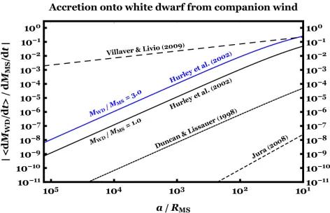
Figure 1. The amount of white dwarf pollution arising from the main sequence star wind as a function of binary separation (a) in units of main sequence star radius (RMS). The labels illustrate
which of equations (12)-(15) have been plotted for each line, and the colours represent the given binary mass ratio. The blue curve could represent, for example, a white dwarf–M dwarf binary.
thenγ(H)≪γ(VL). The expressions forγ(H)andγ(VL) con-tain three degrees of freedom, whereas those for γ(J) and
γ(DL)contain four.
The three degrees of freedom in equations (12) and (14) allow us to plot their entire relevant solution set in Fig. 1. In addition, we plot equations (13) and (15) by assuming a physically plausible value of α = 300δ. These equations and plots can be used to compute the amount of pollution from accretion of the main sequence wind. If at a given time
t = tobs one observes a higher rate of accretion onto the white dwarf than what is predicted from the equations, then likely the excess material arises from accretion of planetary debris. If instead one does not knowa(e.g. the binary system is not resolved) but observes accretion onto the white dwarf, then they could compute a critical separation beyond which pollution arises from planetary systems.
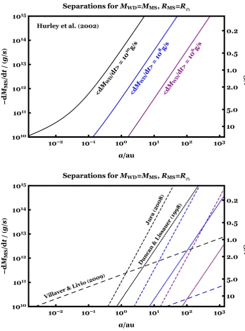
Let us consider this latter case, and plotaas a function of ˙MMSassuming thathM˙WDi ≈106,108,1010 g/s,µ= 1 andRMS=R⊙. The result, in Fig. 2, provides some concrete
examples of the scaled relations. The relevant curves in the lower figure also assume thatRMS= 300RWD.
5.4 The minimum applicable separation
Figure 2. The relation between stellar wind mass loss rate (left y-axis), main sequence stellar age (righty-axis), and binary sep-aration (x-axis) for given values of the averaged white dwarf ac-cretion rate, assumingMWD=MMSandRMS=R⊙. The upper
plot is simply a special case of equation (12) and the Hurley et al. (2002) accretion curve in Fig. 1, while incorporating equation (1). The lower plot, on exactly the same scale, illustrates how other accretion prescriptions (when extrapolated to stellar bina-ries) compare.
6 LINK WITH OBSERVATIONS
We can make comparisons with observations but with the caveat that only some subset of the six variables in equations (8)-(10) are known for each system. In most cases, the white dwarf temperature TWD, white dwarf surface gravity log g (thus massMWDandRWDif necessary), main sequence star massMMSandaare measured. The outstanding question is then, how does one compute the time-dependent variables
˙
MMS(t) andRMS(t)?
6.1 Computing missing variables
If the white dwarf and the companion star were born at the same time (which might not be true for captured compan-ions8), the age of the system can be calculated as the sum
8 This caveat is not particularly important for our considerations,
as captured stars tend to have wider separations than the range which we are predominantly interested in.
of the cooling age of the white dwarft(cool)WD plus the main sequence lifetime of that white dwarft(MSlife)WD :
tobs=t(cool)WD +t (MSlife)
WD . (16)
6.1.1 White dwarf cooling aget(cool)WD
The cooling age may be related to the white dwarf’s lu-minosity through equation 6 of Bonsor & Wyatt (2010) or equation 5 of Veras et al. (2015c) as
LWD
L⊙ ≈
3.26
MWD 0.6M⊙
0.1 +t (cool) WD Myr
!−1.18
(17)
assuming Solar metallicity. The luminosity can then be re-lated to the white dwarf effective temperatureTWD from
LWD=σTWD4 4πR2WD
(18)
where σ is the Stefan-Boltzmann constant. The radius of the white dwarf RWD can be calculated using the white dwarf mass radius relationship (equation 15 of Verbunt & Rappaport 1988):
RWD
R⊙ ≈
0.0127
MWD
M⊙ −1/3
s
1−0.607
MWD
M⊙ 4/3
. (19)
Together, equations (17), (18) and (19) give ust(cool)WD given justMWD andTWD.
6.1.2 Main sequence age t(MSlife)WD
In order to computet(MSlife)WD , we need to employ an initial-to-final mass relation and then a relation between main sequence mass and main sequence lifetime. We do so by creating interpolating functions from theSSEstellar evolu-tion code (Hurley et al. 2000), assuming Solar metallicity, a Reimers mass loss coefficient of 0.5, and the default super-wind prescription of Vassiliadis & Wood (1993). With these assumptions, the only required input into the code is zero-age-main-sequence mass. We created interpolating functions from the resulting grids of values.
6.1.3 Main sequence radiusRMSand mass loss M˙MS
After finally obtaining tobs, we compute M˙MS(tobs) from equation (1) and RMS(tobs) from a different interpolating function from the sameSSEcode.
6.2 An ensemble of systems
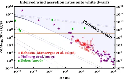
Figure 3. Inferred accretion rates onto white dwarfs from main sequence companion winds from three samples: Holberg et al. (2013), Debes (2006), and Rebassa-Mansergas et al. (2016a). The solid and dashed pairs of curves correspond to the accretion prescriptions in Figs. 1-2 and approximate the boundaries above which (in the shaded area for our fiducial prescription) newly observed polluted white dwarfs would likely have remnant planetary systems, assuming MWD = 0.6M⊙, ˙MMS = −1012 g/s, (black: MMS = 0.6M⊙,
RMS= 0.6R⊙) and (blue:MMS= 0.2M⊙,RMS= 0.2R⊙). The orange horizontal curve roughly represents the current accretion rate
detection limit of 107 g/s. Consequently, if pollution is detected in a white dwarf which is separated from a binary companion by more
than a few au, then very likely the pollution originates from a planetary system.
6.2.1 Holberg et al. (2013) data
The sample from Holberg et al. (2013) contains information aboutMWD,MMS,a and TWD from their Tables 1 and 2. From these values, we can estimate ˙MMS(t) andRMS(t) us-ing the method in Section 6.1. Consequently, we can derive
˙
MWD(t). If white dwarfs in these systems are observed to have values greater than these inferred accretion rates, then our interpretation is that some of that pollution arises from planetary systems.
For this Holberg et al. (2013) sample, we eliminate all systems which (i) lack a data point for at least any one of MWD,MMS,a andTWD and (ii) do not conform to the method outlined in Section 6.1. These cuts leave us with 38 binary systems, which we plot in Fig. 3. The points roughly fall along a diagonal line on the log-log plot, one well ap-proximated by the ˙MMS = −1012 g/s assumption. If ob-served accretion rates are higher than this line, then that material is unlikely to arise from winds, and instead arise from planetary remnants. The figure suggests that observ-ing white dwarfs in binary systems withagreater than a few au for signatures of pollution may be worthwhile if typical accretion rates onto the white dwarf exceed∼107 g/s.
6.2.2 Debes (2006) data
Notably, the Debes (2006) sample includes six stars for which mass loss rates onto the white dwarfs have already been derived; these estimations are not present in the other samples. The rates are indicated by the filled rectangles in
Fig. 3. Three are close binaries, with separations of 0.0073 au (WD 0419-487), 0.013 au (WD 1026+002), and 0.015 au (WD 1213+528), and three are wide binaries, with separa-tions of 1.5 au (WD 0354+463), 28 au (WD 1049+103) and 159 au (WD 1210+464). The wider binaries lie well within the “planetary origin” region of the plot.
6.2.3 Rebassa-Mansergas et al. (2016a) data
remains are the 85 white dwarf-main sequence binaries plotted in Fig. 3.
6.2.4 Curves on the figure
The horizontal orange line represents a typical detectabil-ity threshold of 107 g/s and each accretion prescrip-tion is given by two curves. As with the other figures, the solid curves represent our fiducial prescription from Hurley et al. (2002). The curves with the longest dashes are from Villaver & Livio (2009), the curves with medium dashes are from Jura (2008) and the curves with short dashes are from Duncan & Lissauer (1998). For all pairs,
MWD= 0.6M⊙and ˙MMS=−1012g/s (roughly the current solar value). Within each pair, the black line corresponds to (MMS = 0.6M⊙, RMS = 0.6R⊙) and the blue line to
(MMS= 0.2M⊙,RMS= 0.2R⊙). The difference in the two
solid curves is small enough to be visible only ata∼10−2au. The difference in the curves for the other pairs are more pro-nounced because those prescriptions do not have the same cancellation due to theµ2α2 term.
For a given pair of curves if the observed accretion rates are higher than the curves, then that material is unlikely to arise from winds, and instead arise from planetary rem-nants. Almost all observed systems would therefore contain planetary remnants if the Jura (2008) or Duncan & Lissauer (1998) prescriptions were used. Alternatively, wind accretion could explain atmospheric metals in all but one or two of the observed systems if the Villaver & Livio (2009) prescription is used. We have shaded in the region above the Hurley et al. (2002) curves, the only prescription given here specifically for binary star systems.
We do not believe that the Jura (2008) nor Villaver & Livio (2009) prescriptions (the extreme cases on Fig. 3) – although certainly appropriate in other contexts – are appropriate for our setup, for the following reasons. Jura (2008) assumes accretion only if the target (here the white dwarf) is hit directly. However, the tidal, or Roche, radius of the white dwarf exceeds its physical radius by a factor of several hundred (at a distance comparable to
RMS). On the other end, the accretion radius adopted by Villaver & Livio (2009) is relatively large: on the scale of au (about 1 au for an orbital velocity of 32.5 km/s and about 46 au for an orbital velocity of 4.8 km/s). This formula-tion arises from adopting orbital speed and ignoring wind speed in Villaver & Livio (2009)’s definition of accretion ra-dius. This choice amounts to including factors ofa instead of RMS in the equation. Indeed, if we substituted RMS for their accretion radius, then we would obtain γ(VL)∝α5/2 rather than γ(VL) ∝ α1/2. The other prescriptions lie in-between these two extremes, and the more conservative and stellar-based one is from Hurley et al. (2002).
7 CONCLUSION
The overwhelming focus of planetary debris pollution stud-ies has been single white dwarfs. However, white dwarfs in binary systems may represent an unheralded supplement. Here, we have argued that although the existence of major planets are a near-necessity in systems of single polluted white dwarfs (Section 3), such planets need not exist in
“wide” binary systems containing a polluted white dwarf (Section 4). We then determined just how wide this separa-tion needs to be in order for the origin of the pollusepara-tion to be interpreted as arising from a remnant planetary system (but not necessarily one with a major planet).
This critical separation can be given by one of equations (12, 13, 14, 15) depending on the reader’s preference for ac-cretion physics; we favour, in the context of binary white dwarf / main sequence stars, the conservative but realis-tic prescription from equation (12). We hence find that the critical separation is at most a few au for observed accretion rates of∼107 g/s, the current detectability threshold. We hope our result will encourage observations of white dwarf atmospheres in binary systems, which may provide unparal-lelled insights into binary-star planetary system evolution.
ACKNOWLEDGEMENTS
We thank the referee for their very useful comments. DV thanks ESO Garching for its hospitality during his visit in February 2016. He has received funding from the Euro-pean Research Council under the EuroEuro-pean Union’s Seventh Framework Programme (FP/2007-2013)/ERC Grant Agree-ment n. 320964 (WDTracer). ARM acknowledges financial support from MINECO grant AYA2014-59084-P and by the AGAUR.
REFERENCES
Aannestad, P. A., Kenyon, S. J., Hammond, G. L., & Sion, E. M. 1993, AJ, 105, 1033
Adams, F. C., & Bloch, A. M. 2013, ApJL, 777, L30 Adams, F. C., Anderson, K. R., & Bloch, A. M. 2013,
MN-RAS, 432, 438
Airapetian, V. S., & Usmanov, A. V. 2016, ApJL, 817, L24 Alcock, C., Fristrom, C. C., & Siegelman, R. 1986, ApJ,
302, 462
Alonso, R., Rappaport, S., Deeg, H. J., & Palle, E. 2016, A&A, 589, L6
Althaus, L. G., C´orsico, A. H., Isern, J., & Garc´ıa-Berro, E. 2010, ARA&A, 18, 471
Antoniadou, K. I., & Veras, D. 2016, MNRAS, 463, 4108 Becklin, E. E., Farihi, J., Jura, M., et al. 2005, ApJL, 632,
L119
Bergfors, C., Farihi, J., Dufour, P., & Rocchetto, M. 2014, MNRAS, 444, 2147
Bonsor, A., & Wyatt, M. 2010, MNRAS, 409, 1631 Bonsor, A., Mustill, A. J., & Wyatt, M. C. 2011, MNRAS,
414, 930
Bonsor, A., & Veras, D. 2015, MNRAS, 454, 53
Bonsor, A., Farihi, J., Wyatt, M. C., & van Lieshout, R. 2017, MNRAS, 468, 154
Brasser, R. 2001, MNRAS, 324, 1109
Brown, J. C., Veras, D., & G¨ansicke, B. T. 2017, MNRAS, 468, 1575
Butler, R. P., Wright, J. T., Marcy, G. W., et al. 2006, ApJ, 646, 505
Cassan, A., Kubas, D., Beaulieu, J.-P., et al. 2012, Nature, 481, 167
Croll, B., Dalba, P. A., Vanderburg, A., et al. 2017, ApJ, 836, 82
Debes, J. H. 2006, ApJ, 652, 636
Debes, J. H., & Sigurdsson, S. 2002, ApJ, 572, 556 Debes, J. H., Walsh, K. J., & Stark, C. 2012, ApJ, 747, 148 Desidera, S., & Barbieri, M. 2007, A&A, 462, 345
Dong, R., Wang, Y., Lin, D. N. C., & Liu, X.-W. 2010, ApJ, 715, 1036
Dosopoulou, F., & Kalogera, V. 2016a, ApJ, 825, 70 Dosopoulou, F., & Kalogera, V. 2016b, ApJ, 825, 71 Doyle, L. R., Carter, J. A., Fabrycky, D. C., et al. 2011,
Science, 333, 1602
Dufour, P., Bergeron, P., Liebert, J., et al. 2007, ApJ, 663, 1291
Duncan, M. J., & Lissauer, J. J. 1998, Icarus, 134, 303 Farihi, J., Jura, M., & Zuckerman, B. 2009, ApJ, 694, 805 Farihi, J., Barstow, M. A., Redfield, S., Dufour, P., &
Ham-bly, N. C. 2010, MNRAS, 404, 2123
Farihi, J., Burleigh, M. R., Holberg, J. B., Casewell, S. L., & Barstow, M. A. 2011, MNRAS, 417, 1735
Farihi, J., G¨ansicke, B. T., Steele, P. R., et al. 2012, MN-RAS, 421, 1635
Farihi, J., G¨ansicke, B. T., & Koester, D. 2013a, Science, 342, 218
Farihi, J., Bond, H. E., Dufour, P., et al. 2013b, MNRAS, 430, 652
Farihi, J. 2016, New Astronomy Reviews, 71, 9
Farihi, J., Parsons, S. G., & G¨ansicke, B. T. 2017a, Nature Astronomy, 1, 0032
Farihi, J., von Hippel, T., & Pringle, J. E. 2017b, MNRAS, In Press, arXiv:1707.09474
Fouchard, M. 2004, MNRAS, 349, 347
Fouchard, M., Froeschl´e, C., Valsecchi, G., & Rickman, H. 2006, Celestial Mechanics and Dynamical Astronomy, 95, 299
Frewen, S. F. N., & Hansen, B. M. S. 2014, MNRAS, 439, 2442
Friedrich, S., Jordan, S., & Koester, D. 2004, A&A, 424, 665
Gallet, F., Bolmont, E., Mathis, S., Charbonnel, C., & Amard, L. 2017, In Press A&A, arXiv:1705.10164 G¨ansicke, B. T., Marsh, T. R., Southworth, J., &
Rebassa-Mansergas, A. 2006, Science, 314, 1908
G¨ansicke, B. T., Koester, D., Marsh, T. R., Rebassa-Mansergas, A., & Southworth, J. 2008, MNRAS, 391, L103
G¨ansicke, B. T., Koester, D., Farihi, J., et al. 2012, MN-RAS, 424, 333
G¨ansicke, B. T., Aungwerojwit, A., Marsh, T. R., et al. 2016, ApJL, 818, L7
Gary, B. L., Rappaport, S., Kaye, T. G., Alonso, R., & Hambschs, F.-J. 2017, MNRAS, 465, 3267
Gentile Fusillo, N. P., G¨ansicke, B. T., & Greiss, S. 2015, MNRAS, 448, 2260
Gentile Fusillo, N. P., G¨ansicke, B. T., Farihi, J., et al. 2017, MNRAS, 468, 971
Gurri, P., Veras, D., & G¨ansicke, B. T. 2017, MNRAS, 464, 321
Hadjidemetriou, J. D. 1966, Zeitschrift fr Astrophysik, 63, 116
Hallakoun, N., Xu (#35768#20594#33402), S., Maoz, D., et al. 2017, MNRAS, 469, 3213
Hamers, A. S., & Portegies Zwart, S. F. 2016, MNRAS, 462, L84
Heisler, J., & Tremaine, S. 1986, Icarus, 65, 13
Hermes, J. J., G¨ansicke, B. T., Koester, D., et al. 2014, MNRAS, 444, 1674
Holberg, J. B., Oswalt, T. D., Sion, E. M., Barstow, M. A., & Burleigh, M. R. 2013, MNRAS, 435, 2077
Hollands, M. A., Koester, D., Alekseev, V., Herbert, E. L., & G¨ansicke, B. T. 2017, MNRAS, 467, 4970
Hurley, J. R., Pols, O. R., & Tout, C. A. 2000, MNRAS, 315, 543
Hurley, J. R., Tout, C. A., & Pols, O. R. 2002, MNRAS, 329, 897
Jewitt, D, Hsieh, H., Agarwal, J. 2015, in Michel P., DeMeo F., Bottke W., eds, ASTEROIDS IV, Univ. Arizona Space Science Series
Jura, M. 2006, ApJ, 653, 613
Jura, M., Farihi, J., & Zuckerman, B. 2007, ApJ, 663, 1285 Jura, M. 2008, AJ, 135, 1785
Jura, M., & Xu, S. 2010, AJ, 140, 1129 Jura, M., & Xu, S. 2012, AJ, 143, 6
Jura, M., Xu, S., Klein, B., Koester, D., & Zuckerman, B. 2012, ApJ, 750, 69
Jura, M., & Young, E. D. 2014, Annual Review of Earth and Planetary Sciences, 42, 45
Kepler, S. O., Pelisoli, I., Koester, D., et al. 2015, MNRAS, 446, 4078
Kepler, S. O., Pelisoli, I., Koester, D., et al. 2016, MNRAS, 455, 3413
Kenyon, S. J., & Bromley, B. C. 2017, In Press ApJ, arXiv:1706.08579
Kilic, M., von Hippel, T., Leggett, S. K., & Winget, D. E. 2005, ApJL, 632, L115
Kilic, M., & Redfield, S. 2007, ApJ, 660, 641
Kjurkchieva, D. P., Dimitrov, D. P., & Petrov, N. I. 2017, PASA, 34, e032
Klein, B., Jura, M., Koester, D., Zuckerman, B., & Melis, C. 2010, ApJ, 709, 950
Klein, B., Jura, M., Koester, D., & Zuckerman, B. 2011, ApJ, 741, 64
Kleinman, S. J., Kepler, S. O., Koester, D., et al. 2013, ApJS, 204, 5
Koester, D. 2009, A&A, 498, 517
Koester, D. 2013, Planets, Stars and Stellar Systems. Vol-ume 4: Stellar Structure and Evolution, 4, 559
Koester, D., G¨ansicke, B. T., & Farihi, J. 2014, A&A, 566, A34
Kostov, V. B., Moore, K., Tamayo, D., Jayawardhana, R., & Rinehart, S. A. 2016, ApJ, 832, 183
Kunitomo, M., Ikoma, M., Sato, B., Katsuta, Y., & Ida, S. 2011, ApJ, 737, 66
Li, G., Naoz, S., Valsecchi, F., Johnson, J. A., & Rasio, F. A. 2014, ApJ, 794, 131
Malamud, U., & Perets, H. B. 2016, ApJ, 832, 160 Malamud, U., & Perets, H. B. 2017, ApJ, 842, 67
Manser, C. J., G¨ansicke, B. T., Marsh, T. R., et al. 2016, MNRAS, 455, 4467
Melis, C., Dufour, P., Farihi, J., et al. 2012, ApJL, 751, L4 Mustill, A. J., & Villaver, E. 2012, ApJ, 761, 121
1404
Mustill, A. J., Villaver, E., Veras, D., G¨ansicke, B.T., & Bonsor, A. 2017, In Preparation
Nordhaus, J., & Spiegel, D. S. 2013, MNRAS, 432, 500 Parriott, J., & Alcock, C. 1998, ApJ, 501, 357
Parsons, S. G., Rebassa-Mansergas, A., Schreiber, M. R., et al. 2016, MNRAS, 463, 2125
Payne, M. J., Veras, D., Holman, M. J., G¨ansicke, B. T. 2016, MNRAS, 457, 217
Payne, M. J., Veras, D., G¨ansicke, B. T., & Holman, M. J. 2017, MNRAS, 464, 2557
Petrovich, C., & Mu˜noz, D. J. 2017, ApJ, 834, 116 Pichierri, G., Morbidelli, A., & Lai, D. 2017, In Press A&A,
arXiv:1705.01841
Raddi, R., G¨ansicke, B. T., Koester, D., et al. 2015, MN-RAS, 450, 2083
Rafikov, R. R. 2013, ApJL, 765, L8
Rappaport, S., Gary, B. L., Kaye, T., et al. 2016, MNRAS, 458, 3904
Reach, W. T., Kuchner, M. J., von Hippel, T., et al. 2005, ApJL, 635, L161
Rebassa-Mansergas, A., G¨ansicke, B. T., Rodr´ıguez-Gil, P., Schreiber, M. R., & Koester, D. 2007, MNRAS, 382, 1377 Rebassa-Mansergas, A., Schreiber, M. R., G¨ansicke, B. T.
2013, MNRAS, 429, 3570
Rebassa-Mansergas, A., Ren, J. J., Parsons, S. G., et al. 2016a, MNRAS, 458, 3808
Rebassa-Mansergas, A., Anguiano, B., Garc´ıa-Berro, E., et al. 2016b, MNRAS, 463, 1137
Redfield, S., Farihi, J., Cauley, P. W., et al. 2017, ApJ, 839, 42
Rubincam, D. P. 2014, Icarus, 239, 96
Schatzman, E. L. 1958, Amsterdam, North-Holland Pub. Co.; New York, Interscience Publishers, 1958 Sigurdsson, S., Richer, H. B., Hansen, B. M., Stairs, I. H.,
& Thorsett, S. E. 2003, Science, 301, 193
Staff, J. E., De Marco, O., Wood, P., Galaviz, P., & Passy, J.-C. 2016, MNRAS, 458, 832
Stephan, A. P., Naoz, S., & Zuckerman, B. 2017, In Press, ApJ, arXiv:1704.08701
Stone, N., Metzger, B. D., & Loeb, A. 2015, MNRAS, 448, 188
van Maanen, A. 1917, PASP, 29, 258 van Maanen, A. 1919, AJ, 32, 86
Vanderburg, A., Johnson, J. A., Rappaport, S., et al. 2015, Nature, 526, 546
Vassiliadis, E., & Wood, P. R. 1993, ApJ, 413, 641 Veras, D., Wyatt, M. C., Mustill, A. J., Bonsor, A., &
El-dridge, J. J. 2011, MNRAS, 417, 2104
Veras, D., & Tout, C. A. 2012, MNRAS, 422, 1648 Veras, D., & Wyatt, M. C. 2012, MNRAS, 421, 2969 Veras, D., Hadjidemetriou, J. D., & Tout, C. A. 2013a,
MNRAS, 435, 2416
Veras, D., Mustill, A. J., Bonsor, A., & Wyatt, M. C. 2013b, MNRAS, 431, 1686
Veras, D., & Evans, N. W. 2013, MNRAS, 430, 403 Veras, D., Leinhardt, Z. M., Bonsor, A., G¨ansicke, B. T.
2014a, MNRAS, 445, 2244
Veras, D., Shannon, A., G¨ansicke, B. T. 2014b, MNRAS, 445, 4175
Veras, D., Evans, N. W., Wyatt, M. C., & Tout, C. A. 2014c, MNRAS, 437, 1127
Veras, D., Jacobson, S. A., G¨ansicke, B. T. 2014d, MNRAS, 445, 2794
Veras, D., G¨ansicke, B. T. 2015, MNRAS, 447, 1049 Veras, D., Eggl, S., G¨ansicke, B. T. 2015a, MNRAS, 452,
1945
Veras, D., Eggl, S., G¨ansicke, B. T. 2015b, MNRAS, 451, 2814
Veras, D., Leinhardt, Z. M., Eggl, S., G¨ansicke, B. T. 2015c, MNRAS, 451, 3453
Veras, D. 2016a, Royal Society Open Science, 3, 150571 Veras, D. 2016b, MNRAS, 463, 2958
Veras, D., Mustill, A. J., G¨ansicke, B. T., et al. 2016, MN-RAS, 458, 3942
Veras, D., Carter, P. J., Leinhardt, Z. M., & G¨ansicke, B. T. 2017a, MNRAS, 465, 1008
Veras, D., Georgakarakos, N., Dobbs-Dixon, I., & G¨ansicke, B. T. 2017b, MNRAS, 465, 2053
Verbunt, F., & Rappaport, S. 1988, ApJ, 332, 193 Villaver, E., & Livio, M. 2009, ApJL, 705, L81
Villaver, E., Livio, M., Mustill, A. J., & Siess, L. 2014, ApJ, 794, 3
Voyatzis, G., Hadjidemetriou, J. D., Veras, D., & Varvoglis, H. 2013, MNRAS, 430, 3383
Willems, B., & Kolb, U. 2004, A&A, 419, 1057
Wilson, D. J., G¨ansicke, B. T., Koester, D., et al. 2014, MNRAS, 445, 1878
Wilson, D. J., G¨ansicke, B. T., Koester, D., et al. 2015, MNRAS, 451, 3237
Wilson, D. J., G¨ansicke, B. T., Farihi, J., & Koester, D. 2016, MNRAS, 459, 3282
Wood, B. E., M¨uller, H.-R., Zank, G. P., & Linsky, J. L. 2002, ApJ, 574, 412
Wood, B. E., M¨uller, H.-R., Zank, G. P., Linsky, J. L., & Redfield, S. 2005, ApJL, 628, L143
Wyatt, M. C., Farihi, J., Pringle, J. E., & Bonsor, A. 2014, MNRAS, 439, 3371
Xu, S., Jura, M., Klein, B., Koester, D., & Zuckerman, B. 2013, ApJ, 766, 132
Xu, S., Jura, M., Koester, D., Klein, B., & Zuckerman, B. 2014, ApJ, 783, 79
Xu, S., & Jura, M. 2012, ApJ, 745, 88
Xu, S., Jura, M., Dufour, P., & Zuckerman, B. 2016, ApJL, 816, L22
Xu, S., Zuckerman, B., Dufour, P., et al. 2017, ApJL, 836, L7
Zendejas, J., Segura, A., & Raga, A. C. 2010, Icarus, 210, 539
Zhou, G., Kedziora-Chudczer, L., Bailey, J., et al. 2016, MNRAS, 463, 4422
Zorotovic, M., Schreiber, M. R., G¨ansicke, B. T. 2011, A&A, 536, A42
Zuckerman, B., Koester, D., Reid, I. N., H¨unsch, M. 2003, ApJ, 596, 477
Zuckerman, B., Melis, C., Klein, B., Koester, D., & Jura, M. 2010, ApJ, 722, 725