Volatility and Return Forecasting:
time series and options-based
methods
Submitted in partial ful…lment of the requirements for the degree of
Doctor of Philosophy
by
Xingzhi Yao
Department of Economics
Lancaster University
Acknowledgements
I wish to extend my sincere appreciation to many people for their help and support.
First I would like to thank my supervisors Dr. Marwan Izzeldin and Professor
David Peel for their encouragement, support and academic guidance during these
three and a half years. Particular gratitude goes to Dr. Marwan Izzeldin who has
o¤ered me so many wonderful opportunities to participate in the top workshops
and conferences, and to teach in the econometrics labs and tutorials. I must also
thank Mr. Gerry Steele for very helpful editorial suggestions.
I would like to thank Ms. Caren Wareing and the rest of the administrative
sta¤. A heartfelt thanks to my friends and fellow colleagues who made the
Lancaster experience something special, in particular, Xuguang Li, Summer Guan,
Caroline Khan, Likun Mao, Jinyu Li and Vasileios Pappas. Completing this thesis
without the studentship from the Economic and Social Research Council (ESRC)
would have been impossible.
Lastly and most importantly, I would like to thank my family for their ongoing
love and understanding throughout this period. I am indebted to my best friend,
Xiaoqiang Li, who was always there cheering me up and stood by me through the
good times and bad. Special thanks to my husband, Zhenxiong Li, for his love,
rare patience and company, without whom I would not have been able to balance
Declaration of Authorship
I hereby declare that this thesis is my own work and has not been submitted for
the award of a higher degree elsewhere. Part of the second chapter of this thesis has
been accepted for publication in the Journal of Futures Markets (10.1002/fut.21881),
with my main supervisor, Dr. Marwan Izzeldin, as a second author. In addition
to the second chapter, this thesis contains no material previously published or
written by any other person except where references have been made in the thesis.
Xingzhi Yao
October 2017
I con…rm that 90% of the work, "Forecasting Using Alternative Measures of
Model-Free Option-Implied Volatility", is conducted by Xingzhi Yao.
Marwan Izzeldin
Abstract
This thesis attempts to model and forecast returns and realized volatility using
two di¤erent methods: time series models that exploit the historical information
set and options-based approach that provides a natural forecast of return variation
from listed option prices. Both univariate and multivariate estimation of the time
series models are considered in our analysis.
Chapter 1: This chapter introduces a modi…ed fractionally co-integrated
vector autoregressive model, M-FCVAR, that caters for systems with I(0) and
I(d) variables under the presence of long memory in the co-integrating residuals.
Model inference of the FCVAR and M-FCVAR are compared using Monte Carlo
simulations and an empirical application. The M-FCVAR is found to yield better
in-sample …t and more precise model estimates. Higher return predictability is
observed over long horizons using the M-FCVAR in the empirical example. In
addition, the shocks associated with the I(0) variables could be permanent or
transitory. We show that particular equation speci…cations are required to restrict
these shocks when they produce only transitory e¤ects on the I(d) variables.
The simulation results show that the inappropriate treatment of the shock to the
I(0) variable may negatively a¤ect the precision in the estimation of the model
parameters as well as the in-sample …t.
Chapter 2: This chapter evaluates the performance of various measures of
model-free option-implied volatility in predicting returns and realized volatility.
The critical role of the out-of-the money call options is highlighted through an
volatility. The Monte Carlo simulations show that: …rst, volatility forecasting
performance of measures of implied volatility can be enhanced by employing an
interpolation-extrapolation technique; second, for most measures considered, gains
in their predictive power for future returns can be obtained by implementing an
interpolation procedure. An empirical application using SPX options recorded
from 2003 to 2013 further illustrates these claims.
Chapter 3: This chapter compares the performance of various least absolute
shrinkage and selection operator (Lasso) based models in forecasting future log
realized variance (RV) constructed from high-frequency returns. We conduct a
comprehensive empirical study using the SPY and 10 individual stocks selected
from 10 di¤erent sectors. In an in-sample analysis, we provide evidence for the
invalidity of the lag structure implied by the heterogeneous autoregressive (HAR)
model which has been heavily adopted in volatility forecast. In our out-of-sample
study considering the full time period, the best forecasting performance is usually
provided by the Lasso-based model and the idea of forecast combination tends to
improve the forecasting accuracy of the Lasso-based model. Among all models of
interest, the ordered Lasso AR using the forecast combination serves as the top
performer most frequently in forecasting RV and its improvements over the HAR
model are, in most cases, signi…cant over monthly horizons. Moreover, we observe a
strong impact of the …nancial crisis on the performance of the Lasso-based models.
Nevertheless, the ordered Lasso AR with the forecast combination still retains its
advantages in the post-crisis period, especially over long horizons. In line with the
existing study, the superiority of the Lasso-based models is more evident in a larger
forecasting window size. The conclusions outlined above are not a¤ected by the
variation in the sampling frequency upon which the RV series are based. However,
as the sampling frequency increases, there tends to be more situations where the
Contents
Acknowledgements 1
Declaration of Authorship 2
Abstract 3
Introduction 11
1 A Modi…ed Fractionally Co-integrated VAR for Modelling Systems
with I(d) and I(0) Variables 15
1.1 Introduction . . . 16
1.2 Literature Review . . . 19
1.2.1 Background . . . 19
1.2.2 Fractional Integration and Fractional Co-integration . . . . 21
1.2.3 Testing and Estimation Methods . . . 23
1.3 Methodology . . . 27
1.3.1 Fractional Integration Estimation . . . 28
1.3.2 Fractional Co-integration Estimation . . . 30
1.4 Simulation Study . . . 44
1.5 Empirical Study . . . 46
1.5.1 Data and Volatility Metrics. . . 46
1.5.2 Estimation Results . . . 47
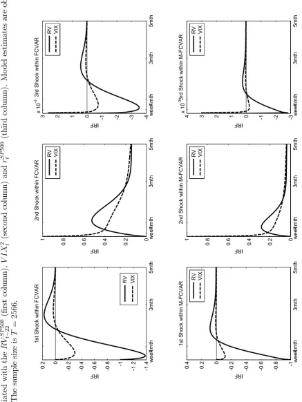
1.5.3 Permanent and Transitory Shocks . . . 53
1.6 Conclusion . . . 55
1.7 Appendix . . . 57
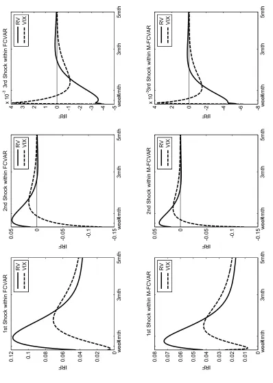
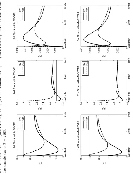
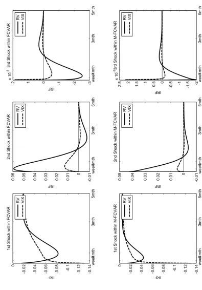
1.7.1 Impulse Response Functions . . . 57
1.7.2 Predictive R-square . . . 60
2 Forecasting Using Alternative Measures of Model-Free Option-Implied Volatility 79 2.1 Introduction . . . 80
2.2 Construction of Volatility Measures. . . 84
2.2.1 Model-Free Implied Volatility and VIX . . . 84
2.2.2 Corridor Implied Volatility . . . 88
2.2.3 Realized Volatility . . . 89
2.3 Error Adjustment Mechanisms . . . 90
2.4 Monte Carlo Simulation . . . 95
2.4.1 Simulation Design . . . 95
2.4.2 Simulation Results . . . 98
2.5 Data. . . 104
2.6 Empirical Results . . . 106
2.7 Conclusion . . . 108
3 Volatility Forecasting Using the HAR and Lasso-based Models: an empirical investigation 126 3.1 Introduction . . . 127
3.2 Literature Review . . . 130
3.2.1 Realized Variance . . . 130
3.2.2 HAR and its extensions . . . 132
3.2.3 Lasso applications in modelling and forecasting RV . . . . 135
3.3 Methodology . . . 137
3.3.1 HAR . . . 137
3.3.3 Lasso-based Estimators . . . 140
3.3.4 Models . . . 147
3.4 Empirical Application . . . 150
3.4.1 Data Description . . . 150
3.4.2 In-Sample Analysis . . . 151
3.4.3 Out-of-Sample Forecast . . . 155
3.5 Conclusion . . . 161
Concluding Remarks 195
List of Tables
1(a) Simulation Results I . . . 61
1(b) Percentage Gains I . . . 62
2(a) Simulation Results II . . . 63
2(b) Percentage Gains II . . . 64
1.3 Summary Statistics . . . 65
1.4 Fractional Integration and Co-integration . . . 65
1.5 S&P 500: variances only . . . 66
1.6 S&P 500 I: variances and returns . . . 67
1.7 S&P 500 II: variances and returns . . . 68
1.8 SPY: variances . . . 69
1.9 SPY I: variances and returns . . . 70
1.10 SPY II: variances and returns . . . 71
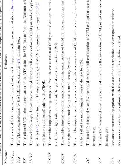
2.1 De…nitions . . . 110
2.2 Simulation Study: summary statistics I . . . 111
2.3 Simulation Study: summary statistics II . . . 112
2.4 Simulation Study: volatility forecast I . . . 113
2.5 Simulation Study: interpolation and extrapolation I . . . 114
2.6 Simulation Study: volatility forecast II . . . 115
2.7 Simulation Study: interpolation and extrapolation II . . . 116
2.8 Simulation Study: return prediction I . . . 117
2.9 Simulation Study: interpolation I . . . 118
2.11 Simulation Study: interpolation II . . . 120
2.12 Empirical Study: summary statistics . . . 121
2.13 Empirical Study: correlation matrix . . . 122
2.14 Empirical Study: volatility forecast . . . 123
2.15 Empirical Study: return prediction . . . 124
3.1 Summary Statistics . . . 163
3.2 Long-Memory Parameters . . . 164
3.3 BIC Criteria . . . 165
3.4 Summary of the OOS Forecast Losses: SPY . . . 166
3.5 Summary of the OOS Forecast Losses: individual stocks . . . 167
3.6 Summary of the Models with the Best Forecasting Performance . . 168
3.7 Summary of the Models Dominating the HAR . . . 169
8(a) OOS Forecast: full sample with 30-sec log RV and RW=1000 . . . . 170
8(b) OOS Forecast: full sample with 30-second log RV and RW=2000 . . 171
8(c) OOS Forecast: pre-crisis period with 30-second log RV . . . 172
8(d) OOS Forecast: post-crisis period with 30-second log RV . . . 173
9(a) OOS Forecast: full sample with 300-second log RV and RW=1000 . 174 9(b) OOS Forecast: full sample with 300-second log RV and RW=2000 . 175 9(c) OOS Forecast: pre-crisis period with 300-second log RV . . . 176
9(d) OOS Forecast: post-crisis period with 300-second log RV . . . 177
10(a)OOS Forecast: full sample with 600-second log RV and RW=1000 . 178 10(b)OOS Forecast: full sample with 600-second log RV and RW=2000 . 179 10(c)OOS Forecast: pre-crisis period with 600-second log RV . . . 180
10(d)OOS Forecast: post-crisis period with 600-second log RV . . . 181
11(a)OOS Forecast: full sample with 30-second log RV and IW . . . 182
11(b)OOS Forecast: full sample with 300-second log RV and IW . . . 183
11(c)OOS Forecast: full sample with 600-second log RV and IW . . . 184
3.12 Estimated AR Coe¢ cients: SPY. . . 185
List of Figures
1.1 Sample Periodograms . . . 72
1.2 Impulse Response Functions I . . . 73
1.3 Impulse Response Functions II . . . 74
1.4 Impulse Response Functions III . . . 75
1.5 Impulse Response Functions IV . . . 76
1.6 Return Predictability: S&P 500 . . . 77
1.7 Return Predictability: SPY . . . 78
2.1 Time Series Plots . . . 125
3.1 Time Series Plots . . . 187
3.2 PACF Plots: full sample . . . 188
3.3 PACF Plots: pre-crisis period . . . 189
3.4 PACF Plots: post-crisis period . . . 190
3.5 HAR vs. adaptive Lasso AR Coe¢ cients . . . 191
3.6 slopeHAR vs. freeHAR AR Coe¢ cients . . . 192
3.7 HAR, cluster group Lasso AR and group Lasso AR Coe¢ cients . . 193
Introduction
Volatility of …nancial time series plays a central role in pricing derivatives, hedging
and computing measures of risk. Volatility forecasting is therefore an important
topic in …nance and …nancial economics, which has held enormous attention of
academics and market investors over the last few decades. The increased availability
of high-frequency data has spurred great interest in the model-free measurement
of variance based upon intraday returns, termed realized variance (RV). On the
other hand, expected returns are considered crucial equity market indicators at
the aggregate market level since they re‡ect the attitudes of investors towards
risk and should carry predictive power for actual future returns theoretically.
However, it still remains controversial in terms of whether equity returns are indeed
predictable. The di¢ culty is that expected returns are not directly observable
and thus one needs to estimate them by means of publicly available information.
This thesis presents various methods to achieve better RV forecast and return
predictions.
Two di¤erent approaches are employed to conduct the forecast of returns and
RV. First, we consider time series models that exploit the historical information set
to formulate return and volatility forecasts in chapter 1 and chapter 3, respectively.
Second, in chapter 2, we concentrate on the market’s expectation of future return
variation from listed option prices, which is perceived as a market based volatility
forecast and may possess information content in predicting future market returns.
Speci…cally, we adopt a model for the analysis of multivariate time series in
the variables. Dynamic dependencies in aggregate stock market returns, implied
and realized volatilities can be well captured by this joint modelling framework.
Univariate time series volatility models are used in Chapter 3 where we apply
several model selection devices to select the relevant lags of the RV for the purpose
of better volatility forecasts. In using the time series models, we account for
the long-memory property of volatility, described by fractional integration and
a slow hyperbolic decay in the autocorrelations. In chapter 1, in addition to
the investigation of long memory of volatilities, we also evaluate their long-run
relationship via both parametric and semiparametric testing methods. In chapter
3, the observed long-memory behaviour is approximated by aggregating across
short-memory heterogenous autoregressive processes. In a departure from chapter
1 and 3, chapter 2 constructs volatility forecasts extracted from combinations
of option prices which do not depend on any pricing formula. Since the option
price incorporates all available information in an e¢ cient market, these model-free
volatility expectations are highly correlated with the future RV and can be seen
as priced risk factors in the cross-section of stock returns.
In chapter 1, we modify the fractionally co-integrated vector autoregressive
(FCVAR) model proposed by Johansen (2008) to allow for the coexistence of
I(0) and I(d) variables under the presence of long memory in the co-integrating
errors. The proposed model is termed the M-FCVAR. We investigate the model
inference of the FCVAR and M-FCVAR in Monte Carlo simulations covering a
wide range of fractional integration orders as well as in an empirical example.
With a more appropriate treatment of theI(0)variable in the system of fractionally
co-integrated processes, the M-FCVAR is found to yield less biased model estimates
and better in-sample …t in the simulation study. In addition to this, we pay
particular attention to the properties of the shocks arising from theI(0) variables
in the (M-)FCVAR framework, which could either be permanent or transitory. The
existing work does not seem to recognize that a particular model design is required
e¤ects on the long-memory variables. Taking into account all the possibilities one
may encounter in practice, we provide equation speci…cations to restrict the shocks
from the I(0) variables. The simulation evidence suggests that one may obtain
biased model estimates and low in-sample …t if the properties of the shocks to the
I(0) variables are incorrectly accounted for. Our empirical application consists of
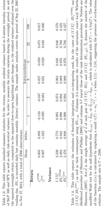
the intraday data for the SPX and SPY indices and the daily data for the volatility
index (VIX), where a joint modelling of the three series, i.e. two fractionally
integrated variances and oneI(0)returns, is implemented in both the FCVAR and
M-FCVAR. With more precise estimates of the model parameters, i.e. fractional
integration order, degree of fractional co-integration and co-integrating vectors,
returns are shown more predictable under the M-FCVAR over long horizons.
Catering for a mixture ofI(0)andI(d)variables, the M-FCVAR can easily …nd
many applications in …nance and …nancial economics. Apart from the example
using the RV, VIX and market returns introduced above, the M-FCVAR can be
further employed to examine the stock market return predictability suggested by
the ‡uctuations in the aggregate consumption-wealth ratio. This is motivated
by the work of Lettau and Ludvigson (2001) who indicate that the aggregate
consumption-wealth ratio can be expressed with regard to several fractionally
co-integrated variables and that the transitory deviations from the common trend
in these variables serve as a strong predictor of future returns.
In chapter 2, we examine the performance of various measures of model-free
option-implied volatility in the forecast of future returns and RV. By decomposing
model-free implied volatility into several components with the use of di¤erent
segments of option strike range, we investigate the role of each component in
the forecasting practice and highlight the importance of the out-of-the money
call options. In addition, we conduct Monte Carlo simulations to ascertain the
impact of discrete strike prices on the forecasting performance of implied volatility
measures. Simulation results show that: …rst, volatility forecast improves with
on the predictive power of implied volatilities for future returns; third, a …ner
partition of strikes leads to better return predictions. These …ndings warrant the
use of an interpolation and extrapolation procedure as an attempt to enhance the
forecasting power of implied volatilities for future RV while only an interpolation
method is needed in return predictions. In the empirical application based on
SPX options from 2003 to 2013, the aforementioned interpolation/extrapolation
procedure is found to signi…cantly enhance the performance of implied volatilities
for forecasting future RV and lead to better return predictions for most measures
in the post-crisis period. The e¤ectiveness of such procedure is also veri…ed in our
simulation study.
In chapter 3, we evaluate the performance of least absolute shrinkage and
selection operator (Lasso) based models in forecasting future RV. The empirical
study adopts the RV series of the SPY and ten individual stocks. We …rst show
that the heterogeneous autoregressive (HAR) model does not fully agree with the
Lasso-type models in terms of the lag structure, which brings into question whether
the HAR is appropriate for modelling and forecasting future volatility. Compared
with the HAR and its extensions, the Lasso-based model usually performs best and
the idea of forecast combination tends to improve the accuracy of the volatility
forecast. Among various Lasso-based models, the ordered Lasso AR using the
forecast combination serves as the top performer most frequently and its gains
over the HAR model are generally signi…cant over monthly horizons. The global
…nancial crisis is found to exert non-trivial impact on the performance of the
Lasso-based models. However, the ordered Lasso AR with the forecast combination
still retains its superiority in the post-crisis period, especially over long forecasting
horizons. We also provide evidence that the Lasso-based models tend to perform
better in a larger window size. Furthermore, as the sampling frequency upon which
the RV series are based increases, the advantages of the Lasso-based models are
Chapter 1
A Modi…ed Fractionally
Co-integrated VAR for Modelling
Systems with
I
(
d
)
and
I
(0)
1.1
Introduction
Many …nancial and economic variables are appropriately described by a fractionally
integrated process, denoted I(d) (e.g. see the discussion and many references in
Nielsen(2010)). In particular, equity and index volatility are well characterized by
anI(d)process (Andersen and Bollerslev(1997) andComte and Renault (1998)).
Implied volatility obtained from option prices displays many of the stylized facts
of equity and index volatility and has been found to be a relevant predictor of
the corresponding asset volatility. Implied volatility, the VIX index in particular,
has featured in a number of volatility forecasting exercises using both short- and
long-memory speci…cations (Bandi and Perron(2006) andBusch, Christensen, and
Nielsen (2011a)). Another use of the implied volatility is to explore the long-run
co-movements between the VIX and the realized volatility of S&P 500, where the
di¤erence between the implied-realized variation measures is termed the ‘variance
risk premium’. This idea has been adopted by Bollerslev et al. (2013) (BOST
hereafter) who are pioneers in predicting stock market returns using a framework
based on the fractionally co-integrated vector autoregressive (FCVAR) model of
Johansen (2008) and Johansen and Nielsen (2012). BOST (2013) show that the
gains of this approach arise from the joint modelling of the multivariate time series
and the capture of the predictability inherent in the variance risk premium.
The FCVAR serves as a direct model of fractional co-integration and provides
a central tool for the analysis of long-run equilibrium relationships among the
I(d) variables. Compared with conventional I(1)=I(0) co-integration, fractional
co-integration allows linear combinations ofI(d)processes to giveI(d b)processes
with d b > 0 and with d and/or b as fractional numbers. The FCVAR has
been applied in several studies. For example: Caporin, Ranaldo, and Santucci
de Magistris (2013) demonstrate the superiority of the FCVAR framework in
forecasting extreme stock prices by accommodating the fractional co-integration
residuals; Rossi and Santucci de Magistris(2013) employ the FCVAR to analyze
the long-run relationship between futures and spot range-based volatility measures;
andJones, Nielsen, and Popiel (2014) exploit the FCVAR to examine the relation
between political support and macroeconomic conditions.
The work of BOST (2013) is uniquely distinctive in that it involves a mixture of
I(d)andI(0) variables. In that presentation, the estimation of the FCVAR model
is simpli…ed by lettingd=b; i.e. there is no memory in the co-integrating residuals.
According to De…nition 2 inJohansen (2008), the FCVAR allows for variation in
the integration order of the variables within the system. Consequently, whend=b,
the inclusion of theI(0) variables is natural in the FCVAR, which is similar to the
coexistence of the I(1) and I(0) variables in the traditional co-integrated VAR.
However, the case ofd > bposes a challenge for the analysis of the FCVAR as the
fractional di¤erencing operator d bis applied, not only to the real co-integrating
vectors, but also to the I(0) variables serving as pseudo co-integrating vectors.
This results in the anti-persistence of the latter. In addition, assumptions need to
be made with regard to the nature of the shocks emanating from theI(0) variables
when they enter the system of the FCVAR model. Theoretically, the impact of the
shocks associated with theI(0)variables can be either permanent or transitory on
theI(d) variables. However, we show that these shocks exert transitory e¤ects in
the FCVAR, only when particular equation speci…cations are adopted; otherwise,
the shocks to theI(0) variables would have nonzero long-run impact on the I(d)
variables. The same interaction between the I(0) and I(1) variables has been
observed by Fisher, Huh, and Pagan (2016) (FHP hereafter) but in a VECM
type of framework. FHP (2016) provide speci…cations for the traditional VECM
that prevent the shocks associated with theI(0)variables from having permanent
e¤ects on theI(1)variables. However, their analysis is limited to situations where
there are equal numbers of exogenousI(1) variables and common factors.
This chapter proposes modi…cations to the FCVAR model ofJohansen (2008)
and I(0) variables when there exists long memory in the co-integrating residuals;
i.e. d > b. Speci…cally, the fractional di¤erencing operator ( d b) is applied to
theI(d)variables within the system prior to the estimation of the FCVAR model.
This procedure does not alter the representation theorem and the calculation of
maximum likelihood estimators of the FCVAR. Without that adjustment, long
memory is induced in the model-impliedI(0)variables, and this may further result
in biased estimates. The chapter also provides the theoretical framework that
outlines the changes required in the speci…cations to restrict shocks arising from
the I(0) variables, so that their e¤ects on the I(d) variables are only transitory.
Complementary to FHP (2016), the chapter covers a variety of situations where
the number of exogenous variables is fewer than or equal to the number of common
factors or where there are only endogenous variables present.
To the best of our knowledge, this chapter is the …rst to consider a modi…ed
FCVAR, henceforth M-FCVAR, to allow for inference and prediction in the presence
of I(0) and I(d) variables. In a simulation study, we show that, compared with
the FCVAR, the M-FCVAR generally yields a better in-sample …t and less biased
estimates of parameters d, b and co-integrating vectors in di¤erent sample sizes.
In addition, the ignorance of the property of the shock arising from the I(0)
variable may damage the precision in the estimation of model parameters and
lower the in-sample …t. The comparison between the FCVAR and M-FCVAR is
also illustrated using an empirical application based on high-frequency data, in
which case market returns are found more predictable over long horizons under
the suggested M-FCVAR.
The rest of this chapter is organized as follows. Section1.2reviews the relevant
literature. Section1.3presents methods adopted in this chapter together with the
M-FCVAR model speci…cations and modi…cations. The Monte Carlo study is
outlined in section 1.4. Section 1.5 describes the data and reports the empirical
results. Section1.6 concludes. Algorithms of the impulse response functions and
1.2
Literature Review
1.2.1
Background
Fractional co-integration, an extension of the co-integration to processes with
fractional degrees of integration, has received substantial research attention recently.
It has been applied in the topics of exchange rates, volatility of …nancial series,
interest rates, electricity prices and political studies, see Gil-Alana and Hualde
(2009) for an overview of the relevant studies. Despite various applications of the
fractional co-integration, the main focus has been on the long-run relationship
between implied-realized volatilities.
Implied volatility is universally considered the best market expectation of the
future volatility over the remaining life of the relevant option. Not surprisingly,
there has been enormous interest in examining the unbiasedness of the implied
volatility forecast of subsequent realized volatility. The relation between the two
volatility proxies can be evaluated via the regression
RV
t = +
IV
t +"t (1.1)
where IV
t denotes implied volatility at timetand RVt represents realized volatility
from t till the option’s expiration time. As noted by Christensen and Nielsen
(2006) and Nielsen (2007), the unbiasedness hypothesis implies a coe¢ cient of
unity. Traditional tests for this hypothesis using the OLS technique generally
result in the conclusion that IV
t provides biased forecast of RVt by obtaining the
slope parameter not equal to one, see Christensen and Prabhala (1998) and
Poteshman(2000).
Realized and implied volatilities are found to display long-memory properties,
seeComte and Renault(1998),Comte, Coutin, and Renault(2012),Ray and Tsay
(2000), Andersen et al. (2001a) and Andersen et al. (2001b), among others. The
in the work of Bandi and Perron (2006), Christensen and Nielsen (2006) and
Nielsen (2007), among others. The presence of fractional co-integration suggests
that both RV
t and IVt are fractionally integrated and that "t in equation (1.1)
is serially uncorrelated or displays short memory. Furthermore, the studies listed
above provide evidence for the long-run unbiasedness, i.e. = 1, using di¤erent
frequency domain methods accounting for the fractional property of the volatilities.
Speci…cally, fractional integration in the region of non-stationarity is found in the
work of Bandi and Perron (2006) whereas the stationary region is indicated in
Christensen and Nielsen (2006) and Nielsen (2007).
It is worth noting that the OLS fails to give consistent estimates of the relation
in equation (1.1) in the case of stationary fractional co-integration. This is due
to the fact that, in such situation, both the regressor and the error exhibit long
memory and thus correlation between them may exist even over long horizons, see
Robinson(1994) andRobinson and Marinucci(2003). In the case of non-stationary
fractional co-integration, the OLS converges slower than the narrow-band least
squares (NBLS) proposed byRobinson(1994), seeRobinson and Marinucci(2001)
and Robinson and Marinucci (2003). In addition, the NBLS leads to consistent
estimates but non-standard limit distributions in the non-stationary range. To
sum up, the earlier …ndings in terms of the biased relation between the two
volatility proxies using the OLS are not reliable since the predictive regression in
(1.1) is usually viewed as stationary fractional co-integration. Similar conclusions
supporting the long-run unbiasedness hypothesis can be found inKellard, Dunis,
and Sarantis(2010) where the integration order of volatility has con…dence intervals
spanning the stationary/non-stationary boundary and Nielsen and Frederiksen
(2011) where the presence of a volatility risk premium, i.e. RV
t IVt , correlated
with implied volatility is accounted for to remove the bias in the NBLS estimator
in regression (1.1).
The di¤erence between the implied and realized variances, the so-called variance
risk aversion, see Bollerslev, Tauchen, and Zhou (2009) andDrechsler and Yaron
(2010), among others. The variance risk premium is found to capture attitudes
toward uncertainty about economic fundamentals and thus predict …nancial market
risk premia and …nancial returns. For instance. Bollerslev, Tauchen, and Zhou
(2009) demonstrate that the variance risk premium is able to capture a nontrivial
fraction of variation in quarterly stock market returns and can result in even greater
return predictability when combined with other conventional predictor variables.
BOST (2013) document a non-trivial return predictability over interdaily and
monthly horizons using the FCVAR model based on 5-minute intraday data. They
also show that the observed strong predictive power for future market returns is
explained by the joint modelling of returns and variances within the FCVAR as
well as the predictability contained in the variance risk premium. Furthermore,
Bollerslev et al.(2014) provide evidence that such pronounced return predictability
suggested by the variance risk premium is not induced by the statistical …nite
sample biases.
Despite the importance of fractional co-integration from both theoretical and
practical perspectives in economics, the testing and estimation of the fractional
co-integrating relation have encountered many di¢ culties. Although the work of
Engle, Lilien, and Robins(1987) provides the concept of common trends between
fractionally integrated processes, subsequent studies are con…ned to situations
where the variables are integrated of order one. Progress in the area of fractional
co-integration is only achieved whenRobinson and Marinucci(2003), Christensen
and Nielsen(2006) andNielsen and Frederiksen(2011), among others develop the
regression-based semiparametric approach to examine whether two long-memory
processes are fractionally co-integrated. Subsequently,Robinson and Yajima(2002)
and Nielsen and Shimotsu (2007) introduce a testing procedure to investigate the
presence of the co-fractional relation by estimating the co-integrating rank of the
matrix of two, or more, fractionally di¤erenced variables. Studies by Johansen
study of fractional co-integration by developing a parametric multivariate FCVAR
model which explicitly captures both the long-run and short-run relationships of
the long-memory processes.
1.2.2
Fractional Integration and Fractional Co-integration
We …rst introduce the fractional integration processes from which the concept of
fractional co-integration stems. Fractional integration describes a strong dependency
between observations which exhibit high persistence that the standard ARMA
framework is unable to capture. This process is neither an I(1) unit root process
nor an I(0) process but rather an I(d) process, where d is between zero and one,
see Baillie (1996) and Robinson (2003) for more details. Assume a covariance
stationary time series Xt with the spectral density f( ). The series Xt is a
long-memory process integrated of orderd (d6= 0) if
f( ) G 2d; as !0+ (1.2)
where G 2 (0;1) is a …nite and nonzero matrix with strictly positive diagonal
elements. The autocovariance functions ofXt decay hyperbolically as shown by
Cov(Xt; Xt ) 2d 1; as ! 1 (1.3)
The parameter d determines the memory of the process. For 0 < d < 0:5; the
series is covariance stationary and contains long memory, implying that shocks
will decay hyperbolically rather than geometrically. By contrast, for0:5< d <1,
the series is no longer stationary, yet still mean reverting. For 0:5< d <0, the
process is stationary but antipersistent, giving rise to the zero spectral density at
the origin frequency instead of in…nity.
Applications of long memory to …nancial and economic data have been extensively
explored with the development of techniques for modelling the fractionally integrated
are the log-periodogram regression of Geweke and Porter-Hudak (1983) and the
local-Whittle likelihood procedure of Kuensch (1987). Both are semiparametric
and thus immune to model mis-speci…cation problems. On the other hand, the
spirit of parametric methods is …rst to build a long-memory model and then to
jointly estimate the model. Popular models are the fractional Brownian motion
proposed byMandelbrot and Van Ness(1968), the fractional white noise and the
autoregressive fractionally integrated moving average (ARFIMA) model developed
byGranger(1980),Granger and Joyeux(1980) andHosking(1981). The ARFIMA
has been heavily employed to capture the long-memory property of the realized
volatility, seeAndersen et al.(2003), Choi, Yu, and Zivot (2010) and Degiannakis
and Floros(2013), among others.
Fractional co-integration generalizes the standard co-integration withI(1)series
and I(0) linear co-integrating relationships by allowing for more ‡exibility in
the order of integration. Speci…cally, fractional co-integration can be de…ned by
assuming two series, yt and xt; which are both integrated of order dx, where dx
can be a fractional number rather than integer one as commonly assumed in the
concept of conventional co-integration, and a linear combination,ut =yt xt; is
I(du). When 0 6du < dx; yt and xt are fractionally co-integrated. In particular,
the model withdx du <0:5 is characterized as weak fractional co-integration by
Hualde and Robinson (2010). Next, we review some recent studies in testing and
estimating the fractional co-integration from di¤erent perspectives.
1.2.3
Testing and Estimation Methods
There is a growing literature devoted to the testing and estimation of fractional
co-integration. A group of contributions is characterized as semiparametric. With
long-run components of each series at origin frequencies, some studies adopt the
regression-based approach to estimate the co-integrating vectors and integration
orders of both regressors and residuals. With the focus on the space of co-integration
rank in the long-memory systems and require no knowledge about the co-integrating
vectors or memory parameters. Parametric maximum likelihood techniques have
also been used to provide the joint estimation of the multivariate fractionally
integrated system. However, there seems no consensus on the optimal testing
procedure for fractional co-integration. One may …nd di¢ culties in having consistent
and conclusive outcome when using di¤erent methodologies. The following section
provides an overview of popular methods of fractional co-integration analysis and
outlines the problems one may encounter in practice.
Semiparametric Approach
A widely accepted procedure is to consider a semiparametric approach characterized
by using a degenerating band of low frequencies for estimation. The semiparametric
approach does not require the accurate speci…cation and estimation of the whole
sample, i.e. it achieves consistency without relying on a parametric model. Two
di¤erent methods in the semiparametric fashion are introduced below, which only
require information related to the behaviour of the spectral density around the
origin.
Regression-Based Approach Regression-based methods generally extend the
work of Engle and Granger (1987) to the case where the order of integration is
not restrictive to integer one, see Marinucci and Robinson (2001) and Gil-Alana
(2003). The key step is to obtain the integration orders of the underlying series
and the regression residuals from the estimated co-integrating relationship and
then to examine whether the persistence reduces or not. The complication of
the regression-based approach is that, unlike the standard situation under OLS
regression, the regressors and the errors may be both stationary and fractionally
integrated and thus are likely to be correlated in the long term. The implication
then is that the OLS estimator is no longer consistent (Robinson(1994),Robinson
(1994) develops a semiparametric narrow-band least squares (NBLS) estimator
in the frequency domain and implements OLS on a degenerating part of the
periodogram around zero frequency, i.e., the so-called narrow-band. In that paper,
Robinson shows that the NBLS estimator is consistent in the stationary case.
Christensen and Nielsen (2006) show that its asymptotic distribution is normal
whendx+du <0:5and when the coherence between regressors and errors is zero
at the origin frequency, i.e. in the long run. The results on the NBLS estimator
for the regressors which are non-stationary long memory are provided byRobinson
and Marinucci (2003); and Chen and Hurvich (2003a) add polynomial trends by
using a tapered NBLS estimator based on di¤erenced data. Concentrating on the
periodogram around the origin, this semiparametric approach enjoys the advantage
of being variant to the short- and medium-run dynamics.
Kellard, Dunis, and Sarantis(2010) improve the NBLS estimator by developing
a new fractional co-integration test which is robust in both the stationary and
non-stationary context. The new estimator is shown to be approximately normally
distributed in …nite sample, which holds across the stationary and non-stationary
regions. Extending the stationary setting ofChristensen and Nielsen(2006) under
a condition of zero long-run coherence between the regressors and co-integrating
errors, Nielsen and Frederiksen (2011) focus on weak fractional co-integration,
including non-stationarity, in the absence of this condition, in which case a bias
term arises in the NBLS estimator. They show that the bias can be estimated
and thus corrected by a fully modi…ed NBLS (FMNBLS) procedure with a careful
choice of bandwidth parameters. The regression-based method is sometimes not
straightforward to implement in empirical studies where integration orders are not
within a particular region as discussed above or where the co-integrating errors
(residuals) are not well de…ned. By contrast, the co-integrating rank test does
not require estimating the co-integrating vector(s) and thus may serve as a good
Spectral Matrix Approach The co-integrating rank test examines the presence
of the co-fractional relation from the perspective of the long-run covariance matrix.
This approach only requires the spectral density matrix at the origin frequency,
but it displays great sensitivity to the selection of bandwidth parameters. Relative
to the regression-based approach, it does not estimate the co-integrating vectors
and only produces a consistent estimate of the co-integrating rank. The estimate
of the rank greater than one and less than the number of variables indicates the
existence of the co-fractional relation. Hence, this approach is not appropriate
when speci…c information about the co-fractional relation, e.g. strength of the
relation, is required.
Robinson and Yajima(2002) are the pioneers in implementing the co-integrating
rank estimation in the region of stationarity. Chen and Hurvich(2003b) investigate
the rank of an averaged periodogram matrix of tapered and di¤erenced observations
and …x the number of frequencies used in the periodogram averages as the sample
size increases, which applies to both stationary and non-stationary situations.
Their assumption of strictly positive rank is relaxed in subsequent work by Chen
and Hurvich (2006) who consider the null of no fractional co-integration, i.e.
rank equal to zero. Nielsen and Shimotsu (2007) also attempt to accommodate
(asymptotically) stationary and nonstationary fractionally integrated processes.
They use the exact local Whittle analysis ofShimotsu and Phillips (2005), which
generalizes the local Whittle estimator of Kuensch (1987) to allow for any value
of the memory parameter d. The estimate of co-integrating rank is achieved by
examining the rank of the spectral density matrix of the dth di¤erenced processes
around the zero frequency.
Parametric Approach
A fully parametric approach is more e¢ cient in using the entire sample instead
of focusing on the origin frequency of the periodogram only. However, it shows
I(1)=I(0) co-integration, the standard tool to handle the relationship among the multivariate time series is the vector error correction model (VECM) as introduced
byEngle and Granger(1987). The representation is given by
Xt= 0Xt 1+ ik=1 i Xt i+"t (1.4)
where Xt is p dimensional I(1) series and "t is p dimensional independent and
identically distributed (i.i.d.) with mean zero and covariance matrix .
Multivariate score tests (or Lagrange multiplier tests) for fractional integration
have been developed by Johansen (1995) and Nielsen (2005), as a prerequisite
for further detailed investigation of fractional co-integration. Substantial e¤orts
have since been made to improve and optimize the parametric estimation of the
fractional co-integration. The most famous model is the Fractionally Co-integrated
Vector Autoregressive (FCVAR) model (or the so-called Fractional Vector Error
Correction model (FVECM) in some studies) proposed by Johansen (2008) and
further analyzed by Johansen and Nielsen(2012).
Some important studies related to the development of the parametric framework
for fractional co-integration include: Breitung and Hassler(2002) suggest a test for
the rank of fractional co-integration in the FCVAR while assuming the integration
order is known and that the errors are i.i.d. Gaussian; Avarucci and Velasco
(2009) introduce the Wald test to determine the co-integration rank in a system of
nonstationary fractionally integrated variables within the FCVAR-type framework;
×asak (2010) considers a pro…le likelihood method to estimate the parameters of
theGranger(1986) model and to test for the null hypothesis of no co-integration.
This estimation method has been extended by Johansen and Nielsen (2012) to
the FCVAR model; Franchi (2010) investigates a richer co-fractional structure by
extending the representation theory of the FCVAR model inJohansen(2008); and
×asak and Velasco(2015) introduce a novel two-step procedure for co-integrating
rank estimation, which allows di¤erent co-integration relations to display di¤erent
Johansen and Nielsen(2012). Essentially the FCVAR is derived by replacing the
lag and di¤erence operators in the VECM model with their fractional counterparts.
It has been adopted by BOST(2013),Jones, Nielsen, and Popiel(2014),Dolatabadi,
Nielsen, and Xu (2015) and Dolatabadi, Nielsen, and Xu (2016), among others.
It exhibits the advantage of allowing for multivariate analysis, ‡exible selection of
parameters and good performance in forecasting.
A mixture of variables with di¤erent integration orders in the analysis of
fractional co-integration is frequently encountered in practice. The study by
FHP (2016) considers a VECM model with both I(1) and I(0) variables but
little work has been done in the FCVAR framework with the coexistence of I(d)
and I(0) variables. FHP(2016) classify the shocks arising from the I(0) variables
into the permanent and transitory, termed the P0 and T0 shocks. They show
that, in a system containing I(0) and I(1) variables which are co-integrated,
the co-integration may no longer exist when the T0 shocks become P0 shocks.
A device is suggested by FHP(2016) to calculate the permanent component of
theI(1) variables when the shocks associated with the I(0) variables have either
transitory or permanent e¤ects on the I(1) variables. Furthermore, in order to
restrict the shocks from the I(0) variables to exert only transitory impact on
the other variables, they show that the true error correction terms and the I(0)
variables must appear as di¤erences in the equations of the VECM where the
response variables are permanent components. However, their work is con…ned
to the situation where there are equal numbers of exogenous I(1) variables and
common factors, i.e. permanent components.
1.3
Methodology
The following section presents the methods adopted in this chapter. We employ
the FCVAR model to accommodate the system ofI(d)variables. When moving to
the co-integrating error. Properties of the shocks arising from the I(0) variables
are also accounted for in various situations. As an attempt to overcome the
identi…cation problem of the (M-)FCVAR, we obtain the fractional integration
estimate using the exact local Whittle estimator ofShimotsu and Phillips (2005).
The presence of fractional co-integration is examined using the exact local Whittle
rank test byNielsen and Shimotsu (2007) coupled with a modi…ed Wald test for
the equality of the orders of fractional integration.
1.3.1
Fractional Integration Estimation
Fractional co-integration originates from several variables exhibiting long-memory
properties. Hence, we …rst introduce the procedure of estimating the order of
fractional integration, which serves as the basis for the subsequent analysis of
co-fractional relations. A fractionally integrated process is de…ned as I(d) if its
dth di¤erence is integrated of order zero, wheredcan be any real number. In spite
of a number of approaches proposed to estimate the long-memory parameter d,
the semiparametric procedure has long been widely explored and applied since it
requires no assumptions about the short-run dynamics and thus stays robust to
mis-speci…cation problems. This chapter adopts the exact local Whittle estimator
ofShimotsu and Phillips(2005), which extends the work of local Whittle analysis
by Kuensch (1987) and Robinson (1995) to allow for any value of the fractional
di¤erencing parameter,d.
To de…ne the frequency-domain local Whittle estimator, we assume that a
process Xt has the spectral density, f( ), de…ned in equation (1.2). Let the
fractionally integrated Xt be generated by the model
d
Xt= (1 L)dXt= t1ft>1g; t= 0; 1; ::: (1.5)
where 1f:g represents the indicator function, L is the lag operator and t is
assumed to be a covariance stationary process whose spectral density, f ( ), is
for 0 (Robinson (1995)). An alternative representation of Xt based on
1; :::; n can be derived by inverting and expanding the equation (1.5),
Xt = d t1ft >1g (1.6)
= (1 L) d t1ft>1g
The discrete Fourier transform (DFT),!x( j);and the periodogram,Ix( j)ofXt,
t=1, ,T at the fundamental frequencies can be written as
!x( j) = (2 T) 1=2 Tt=1Xteit j; j =
2 j
T ; j = 1; :::; m <
T
2 (1.7)
Ix( j) = j!x( j)j
2
One advantage of semiparametric estimation over the parametric approach is
that it employs frequencies near the origin only and treats the periodogram away
from the zero nonparametrically. The conventional local Whittle (LW) estimator
byKuensch(1987) andRobinson(1995) relies on the Gaussian objective function,
Qm(G; d) =
1
m m
j=1[log(G 2d
j ) +
2d j
G Ix( j)] (1.8)
where j = 2Tj; j = 1; :::; m < T2:The LW estimate is thus derived by minimizing
the function Qm(G; d). Robinson (1995) proves that the asymptotic standard
errors of the LW estimator are pm(dT;mb d))N(0;14):In spite of its enhanced
e¢ ciency over the GPH estimator (Geweke and Porter-Hudak (1983)) within the
stationary region, both GPH and LW estimators display nonstandard behaviour
whend > 34 (Kim and Phillips (2006)).
Shimotsu and Phillips(2005) provide a procedure which can be applied in the
stationary and nonstationary regions and it estimates (G; d) by minimizing the
objective function
Qm(G; d) =
1
m m
j=1[log(G 2d
j ) +
1
whereI dx( j)is the periodogram of dXt. ConcentratingQm(G; d)with respect
toG, we obtain the exact local Whittle (ELW) estimator given by
e
d= arg min
d2[ 1; 2]
R(d) (1.10)
where 1 and 2 are the lower and upper bounds of the admissible values of d
and
R(d) = logGb(d) 2d1 m
m
j=1log j (1.11)
b
G(d) = 1
m m
j=1I dx( j)
This ELW estimator has been proved to be consistent and asymptotically normally
distributed when the underlying value ofd 2( 1; 2) and 2 1 92 with the
mild assumptions on bandwidthm and stationary t:
The desirable properties of the ELW estimator byShimotsu and Phillips(2005)
are based on the assumption that Xt is generated by the process in equation
(1.5) and that the mean/initial value of the process is known. When the series
is accompanied by a linear time trend or an unknown mean/initial condition, a
more appropriate choice of estimation is the two-step ELW estimator byShimotsu
(2010). However,Shimotsu (2010) indicates that the ELW estimator byShimotsu
and Phillips(2005) remains consistent ford2( 12;1)and is asymptotically normal
ford2( 12;34)if the unknown mean is replaced by the sample average. In our case,
the memory estimates of the variance series considered in the empirical study are
within the standard region of ELW estimation, and thus we carry out the empirical
1.3.2
Fractional Co-integration Estimation
Exact Local Whittle Rank Test
Before moving to the modelling and estimation of the fractional co-integration
by the FCVAR, we obtain the estimate of the co-integration rank based on an
exact local Whittle approach. Speci…cally, we determine the co-integrating rank
of the spectral density matrix of the dth di¤erenced process around the origin
frequency. This procedure is …rst proposed by Robinson and Yajima (2002) and
later extended by Nielsen and Shimotsu (2007), who account for both stationary
and non-stationary situations.
Robinson and Yajima (2002) stress that the test for homogeneity of orders of
fractional integration could deliver misleading conclusions if the co-integration is
not accounted for. Hence, we start the analysis by …rst estimating the co-integrating
rank. Assume there is a p-vector fractional process Xt where each element is
fractionally integrated of order d1; :::; dp, respectively. The work of Nielsen and
Shimotsu (2007) builds on the assumption of equal integration orders and thus
d1; :::; dp are represented by d , where de = p1Ppa=1dab with each dab given by
equation 1.10. The consistent estimator of the spectral density at the origin is
given by
b
G(d ) = 1
m1
m1
X
j=1
Re[I (L;d ;:::;d )x( j)] (1.12)
where j = 2Tj and I (L;d ;:::;d )x( j) is the periodogram of ( d X1t;:::; d Xpt)0:
Here,Gb(d )uses a new bandwidth parameter m1 instead ofmpresent in equation
(1.8). Letba be theath eigenvalues ofGb(d )and the co-integration rank r can be
determined by following the procedure ofRobinson and Yajima (2002)
b
r = arg min
u=0;:::;p 1L(u) (1.13)
L(u) = v(T)(p u)
p u
X
a=1
wherev(T) should be positive and meet the assumption as follows
v(T) + 1
m11=2v(T) !0 (1.14)
Nielsen and Shimotsu (2007) show that a higher rank estimate is more likely to
be selected when a largerv(T)is applied. In order to obtain a more conservative
estimate ofr, we choose to employ a small v(T) =m10:4.
Once the presence of the co-fractional relation has been investigated by the rank
estimation, we can examine the equality of the orders of fractional integration by
testing the nullH0 :da=d ; a= 1; :::p. The test statistic is given by
b
T0 =m(Sdb)0(S
1 4Db
1
(Gb Gb)Db 1S0 +h(T)2Ip 1) 1(Sdb) (1.15)
where represents the Hadamard product,S = [Ip 1; ]0, is the (p 1)-vector of
ones,h(T) = 1=log(T)is of more frequent application, andDb =diag(Gb11; Gbpp).
The memory estimates dbof variables in the vector are derived by the univariate
exact local Whittle estimator by Shimotsu and Phillips (2005), with m Fourier
frequencies being employed. The selection of parameters, (m; m1; v(T)); will be
speci…ed in our empirical example. If variables are not fractionally co-integrated,
b
T0 !d 2(p 1); while Tb0 !p 0 if they are co-integrated.
The FCVAR model
To further examine the long-run and short-run dynamics among the fractionally
integratedI(d)variables, we adopt the framework byJohansen(2008) andJohansen
and Nielsen(2012). Consider a vectorXt2I(d)containingpelements, the FCVAR
model is in the form of
dX
t= 0 d bLbXt+
k
X
c=1
where "t is p dimensional i:i:d:(0; ). Let Lb = 1 b be the fractional lag
operator and d be the fractional di¤erence operator with d= (1 L)d
(1 L)d = 1
X
i=0
i(d)Li; with i(d) = ( 1)i d
i =
( d+i)
( d) (i+ 1) (1.17)
= 1 dL+d(d 1) 2! L
2 d(d 1)(d 2)
3! L
3+
where (:) is the gamma function. The error correction term is denoted by
0 d bXt, where is a (p r)matrix consisting of r co-integrating vectors and r
is the so-called co-integration rank. The linear combination 0Xt is integrated of
order (d b) with d b > 0. This suggests that the co-integrating combination
reduces the integration order ofXt byb, whereb measures the degree of fractional
co-integration. The matrix is of order (p r) and contains the parameters
representing the speed of adjustment towards long-run equilibrium. The short-run
dynamics are measured by the lag coe¢ cients( 1; : : : ; k).
The FCVAR model is estimated by means of a pro…le likelihood technique (see
Johansen and Nielsen (2012)). The maximum likelihood estimators (MLE) and
maximized likelihood are calculated by minimizing the pro…le likelihood`( ; r)as
a function of = (d; b). Onced and b are determined, all the other parameters,
b, b, and bc for c = 1; ; k can be concentrated out by regression and reduced
rank regression. Recall the FCVAR in equation (1.16) and de…ne Z0;t = dXt;
Z1;t = ( d b d)Xt and Zk;t = dLcbXt
k
c=1. For …xed = (d; b), the MLE is
found by reduced rank regression ofZ0;tonZ1;tcorrected forZk;t. More speci…cally,
we need to obtain the residuals of the respective regressions ofZ0;t andZ1;t onZk;t,
denoted as R0;t and R1;t, to construct the pro…le likelihood function `( ; r). In
the conventional situation where all the variables are fractional of order d, the
regression of Z0;t on Zk;t is balanced in the sense that both the regressand and
regressor areI(0), while the regression of Z1;t onZk;t is not balanced with theI(b)
regressand and I(0) regressor, i.e. a reduction of b in the integration order from
have the largest squared partial correlations withZ0;t after correcting for fractional
lags.
The likelihood ratio (LR) test can be used to determine the co-integration
rank r. Letting = 0, we have the LR test statistic of the null hypothesis
Hr :rank( ) =r against the alternative Hp :rank( ) =p: The pro…le likelihood
function is maximized both under the null and alternative hypothesis and then the
LR test statistic is such that
LRT(q) = 2 log(`(bp; p)=`(br; r)) (1.18)
where `(bp; p) = max `( ; p); `(br; r) = max `( ; r) and q = p r. Johansen
and Nielsen(2012) show that LRT(q)depends heavily on the parameter b in that
8 > < > :
LRT(q)! 2(q2); 0< b <1=2 (weak fractional co-integration)
LRT(q) non-standard, b >1=2 (strong fractional co-integration)
(1.19)
Due to the non-standard asymptotic distribution of the test statistic in the case of
strong fractional co-integration, we follow the program developed byMacKinnon
and Nielsen (2014) to obtain the asymptotic P values for the LR co-integrating
rank tests. In addition, the selection of lag valuek is of critical importance in the
speci…cation of the FCVAR model. We determine the order of lag by following
theBIC information criteria while ensuring that the short-run coe¢ cients k are
signi…cantly di¤erent from zero and that the residuals are stationary and serially
uncorrelated.
A crucial problem of the FCVAR model is the lack of identi…cation on the
likelihood function as suggested byCarlini and Santucci de Magistris (2017), i.e.,
there may exist equivalent sub-models associated with di¤erent sets of parameters.
When the lag order, k, is unknown and potentially over-speci…ed, Carlini and
Santucci de Magistris (2017) present a strong relationship between the lag length
condition for identi…cation of the FCVAR model corresponding to any lag structure.
Such condition,F(d), is de…ned by
j 0? ?j 6= 0 (1.20)
where 0? = 0, and =I Pkc=1 c. When the cointegrating rank is unknown,
they further show that the FCVAR with full rank and k lags is equivalent to
that with rank 0 and k + 1 lags, in which case the F(d) condition delivers no
information in terms of the model identi…cation. Whether the rank is known or
not, the identi…cation issue for any lag greater than one can be solved by imposing a
lower-bound restriction ondwhere the lower bound is based upon a semiparametric
estimate, e.g. the estimator by Shimotsu and Phillips (2005), of the integration
order, termed as the de. The lower bound min is given by
min =de c de (1.21)
where c= 0:15 is recommended in the work ofCarlini and Santucci de Magistris
(2017).
The M-FCVAR model
This section introduces the M-FCVAR model and provides the speci…cations which
ensure that the shocks associated with the I(0) variables do not exert long-run
e¤ects on theI(d)variables.
The FCVAR in equation (1.16) does not require that all components of Xt
exhibit the same order of integration, which accords with the situation where there
can be a mixture ofI(1)and I(0)variables in the traditional VECM. For instance,
I(0:4) variables,X1t and X2t, and one I(0) variable, X3t, given by
X1t = +0:4"1t +0:2"2t+"3t (1.22)
X2t = +0:4"1t+ +0:2"2t+"3t
X3t = "1t+"2t+"3t
where Xt = (X1t, X2t, X3t)0, "t is i.i.d. (0, I3) and +d"t = Pit=01( 1)i id "t i.
The long-run transfer function for 0:4X
t, i.e. the matrix of responses of the
variables to the shocks, is
C(1) =
0 B B B B @
1 0 0 1 0 0 0 0 0
1 C C C C A
and the spectrum is C(1)0C(1) 6= 0. Hence, 0:4X
t 2 F(0) and Xt 2 F(0:4)
according to De…nitions 1 and 2 in Johansen (2008), which suggests that the
representation theorem and the properties of MLE of the FCVAR remain unchanged
when the I(0) variables are introduced into the system of fractional variables.
The following section gives an outline of the problem that may arise when the
FCVAR in equation (1.16) is used to accommodate a system containingI(d)and
I(0) variables. As a standard method employed in the literature of treating an
I(0) variable in the VECM, we adopt the idea of ‘pseudo’co-integrating relation.
Speci…cally, we involve the extra co-integration vector being unit vector with unity
in the position corresponding to the I(0) variable and zeros elsewhere. Without
loss of generality, we assume that there aren I(d)variables and q I(0) variables in
Xt which containsp elements, giving p=n+q. Among the I(d) variables, there
arer co-integrating relations and thusl =n rpermanent components. Here, we
refer to therco-integrating relations as ‘true’co-integrating relations, as opposed
to theq ‘pseudo’co-integrating relations that arise from the I(0) variables, which
are treated as ‘fractionally co-integrated with themselves’. We let Xt = (x1t, x2t,
as endogenous or weakly exogenous variables in the subsequent analysis andx3t is
theq 1 vector ofI(0) variables. We then construct
=
0 B B B B @
1 1
2 2
3 3
1 C C C C A
p (r+q)
0 =
0 B @
0
1 02 0
0 0 Iq
1 C A
(r+q) p
(1.23)
The …rst row of block matrices in 0 are the coe¢ cients in the ‘true’co-fractional
relations among I(d) variables, while those in the second row correspond to the
‘pseudo’ co-fractional relations. The FCVAR in equation (1.16) is no longer
appropriate for modelling a system containing a mixture ofI(d)andI(0) variables
when d > b, in which case the term 0 d bX
t contains anti-persistent error
correction terms, i.e. terms which are integrated of a negative order, due to the
presence ofI(0)variables inXt. The mis-speci…cation problem can also be seen by
considering the representation theorem of the FCVAR (1.16). Given and as
de…ned in equation (1.23) and =I Pkc=1 c, the matrixC= ?( 0? ?) 1 0?
contains only zeros in the lastq rows corresponding to the q I(0) variables inXt.
Following the work ofJohansen and Nielsen(2012), the FCVAR in equation (1.16)
has the solution
Xt=C +d"t+
(d b)
+ Yt++ t (1.24)
ford 1=2where the operator +d is used to de…ne a nonstationary process and
Yt is fractional of order zero. The solution of the FCVAR model for the last q
equations, i.e. I(0) x3t, then reduces to
x3F CV ARt =e30 +(d b)Yt++e30 t (1.25)
wheree30 = (0
q n; Iq q). It is clear that thexF CV AR3t is integrated of order(d b),
which erroneously exhibits long memory if d > b due to the mis-speci…cations.
This problem remains in the case of d < 1=2 where the solution of the FCVAR
The M-FCVAR is developed to address the issue described above. We apply
the fractional di¤erencing operator d b to each of the long-memory variables in
Xt and construct a new system Xt. Adapting the notation of the FCVAR, we
obtain the M-FCVAR as follows
bX
t = 0LbXt +
k
X
c=1
c bLcbXt +"t (1.26)
Here, the M-FCVAR di¤ers from the FCVAR only in the way that the fractional
I(d)variables have been transformed to I(b)variables. Hence, the representation
theorem of the M-FCVAR in equation (1.26) is the same as that of the FCVAR
except that d is always equal to b. We can then show that the M-FCVAR
model-implied xM3t F CV AR remains I(0) according to equation (1.25) sinced =b.
Both the FCVAR and M-FCVAR are estimated by means of a pro…le likelihood
technique (see Johansen and Nielsen (2012)). For each …xed combination of
= (d; b)in the estimation of the M-FCVAR, we …rst construct Xt by applying
(d b) to the fractionally integrated variables in X
t. We then de…ne Z0;t = bXt;
Z1;t = (1 b)Xt and Zk;t = bLcbXt
k
c=1. The MLE is found by reduced rank
regression of Z0;t onZ1;t corrected for Zk;t.
For the case of the coexistence of I(d) and I(0) variables in the system of the
(M-)FCVAR, there will be shocks coming from the I(0) variables. The e¤ects of
those shocks can either be transitory or permanent on the I(d) variables. In the
rest of this section, we show that the shocks associated with the I(0) variables
produce zero long-run impact on the fractional variables only when a particular
model design is considered. We follow the approach of FHP (2016) to control
for the long-run e¤ects of theI(0) variables and extend their work by allowing for
variation in the number of weakly exogenousI(d)variables within the (M-)FCVAR
framework.
For simplicity, we consider the M-FCVAR with only one lag(k = 1) as follows
bX
We start with the case where only n I(d) variables, x1t and x2t, are present in
the M-FCVAR. Applying the operator d b to x
1t and x2t, we obtain Xt = (x1t,
x2t)0 which is fractionally integrated of order b. We de…ne 0
true = 1 2
and its orthogonal complement 0
true? = as a l n matrix, which
gives 0true? true = 1 + 2 = 0. There are a number of di¤erent ways of
de…ning the common stochastic trend. Here, we follow Gonzalo and Granger
(1995) in estimating the permanent and transitory (PT) components ofXt. As in
equation (1.27), Xt can be explained with regard to a smaller number, l=n r,
of I(b) variables, de…ned as common factors ft = 0true?(x1t, x2t)0 and r I(0)
variables zt = 0(x1t, x2t)0 conditional on that ( 0true?, )0 is nonsingular. The
Gonzalo and Granger(1995) de…nition requires the I(b) common factors ft to be
linear combinations of the observable variables and also requires that zt does not
Granger-causeftin the long run. The PT approach exhibits two main advantages
such as: (1) ft is unique and can be easily obtained from the (M-)FCVAR;
(2) hypothesis testing on the common trends is straightforward and follows a
chi-square distribution. TheGonzalo and Granger(1995) decomposition has been
widely applied in various studies such asBaillie et al.(2002),Banerjee, Marcellino,
and Osbat(2004),Blanco, Brennan, and Marsh(2005),Bollerslev et al.(2013) and
Dolatabadi, Nielsen, and Xu(2015), among others.
We then add x3t, the q 1 I(0) variables, into the system of the M-FCVAR
and adopt and speci…ed in equation (1.23). The ‘true’error correction term,
t, is given by
t = 01x1t+ 02x2t (1.28)
and the ‘pseudo’error correction term is x3t.
Proposition 1 In the equations of the M-FCVAR (1.26) where theI(b)dependent
variables constitute the common component, the ‘pseudo’error correction term,x3t
in levels form, is not present, which ensures that shocks associated with x3t have