See discussions, stats, and author profiles for this publication at: https://www.researchgate.net/publication/303738583
Cross-validation aggregation for combining
autoregressive neural network forecasts
Article in International Journal of Forecasting · June 2016
DOI: 10.1016/j.ijforecast.2015.12.011
CITATIONS
2
READS
68
2 authors:
Devon K. Barrow
Coventry University
14PUBLICATIONS 117CITATIONS SEE PROFILE
Sven F. Crone
Lancaster University
67PUBLICATIONS 993CITATIONS SEE PROFILE
All content following this page was uploaded by Devon K. Barrow on 02 June 2016.
1
Cross-validation aggregation for combining
autoregressive neural network forecasts
Devon K. Barrow1 and Sven F. Crone2
1School of Strategy and Leadership, Coventry University, Priory Street, Coventry, CV1 5FB 2
Lancaster University Management School, Department of Management Science, Lancaster, Lancashire, LA1 4YX, UK
Abstract
This paper evaluates k-fold and Monte Carlo cross-validation and aggregation (crogging) for
combining neural network autoregressive forecasts. We introduce Monte Carlo crogging which
combines bootstrapping and cross-validation in a single approach through repeated random splitting
of the original time series into mutually exclusive datasets for training. As the training/validation
split is independent of the number of folds, the algorithm offers more flexibility in the size, and
number of training samples compared to k-fold cross-validation. The study also provides for
crogging and bagging: (1) the first systematic evaluation across time series length and combination
size, (2) a bias and variance decomposition of the forecast errors to understand improvement gains,
and (3) a comparison to established benchmarks of model averaging and selection. Crogging can
easily be extended to other autoregressive models. Results on real and simulated series demonstrate
significant improvements in forecasting accuracy especially for short time series and long forecast
horizons.
Key words: Forecast combination; bootstrapping, Monte Carlo, time series, cross-validation autoregression
1
Corresponding author. Tel.: +44 (0) 779 626 76 74
Email address: [email protected] (D.K. Barrow).
2
1.
Introduction
Improving the accuracy of a univariate time series forecast remains important in many
disciplines, from environmental sciences to business and finance. The approach of combining
multiple forecasts has shown particular promise (Clemen and Winkler 1986; Timmermann
2006) as evidenced by various empirical studies (Aksu and Gunter 1992; Macdonald and
Marsh 1994; Stock and Watson 2004; Clements and Hendry 2007; Jose and Winkler 2008;
Kourentzes, Barrow, and Crone 2014) and objective forecasting competitions (Makridakis et
al. 1982; Makridakis and Hibon 2000). The traditional approaches to forecast combination
typically involve a set of independent, pre-specified forecasts from different algorithms,
which are combined in a second step using a variety of different weighting schemes.
As an alternative to combining predictions of different algorithms, research in
machine learning for predictive classification routinely apply repeated subsampling of the
dataset on which a single algorithm is parameterised, creating diversity in data rather than in
algorithms. Most widely studied, bagging (Breiman 1996a) and k-fold cross-validation
ensembles (Krogh and Vedelsby 1995) adopt different data resampling techniques,
bootstrapping and cross-validation respectively, to actively create diverse estimates of the
same base learner algorithm for successive combination of the predictions. Their success in
improving performance and robustness of predictions in classification has been empirically
proven in a large number of research studies (see e.g. Dietterich 2000; Zhou, Wu, and Tang
2002), with their wide use reflected in published textbooks (see e.g. Perrone and Cooper
1992) and their availability in standard software packages (see e.g. Matlab and Salford
Predictive Modeler Software Suite).
Despite both methods having been extended to regression in general, and time series
forecasing in particular, this class of algorithms has received relatively limited attention in
3
Donate et al (2013) and Soric and Lolic (2013) studied cross-validation for time series
forecast combination, with promising results (Donate et al. 2013; Sorić and Lolić 2013).
However, both studies were constrained to the variant of k-fold cross-validation, applying a
fixed and predetermined number of subsamples to create diversity. In contrast Monte Carlo
cross-validation which combines the benefits of both cross-validation and bootstrapping –
repeated random sampling with replacement – in a single approach has been relatively
ignored for forecast combination.
In this study we use cross-validation for combining autoregressive forecasts. The
forecast combination averages over a set of forecast models trained using mutually exclusive
cross-validation replicates, sampled from a given learning set. Within the general framework
of cross-validation and aggregating, or crogging for short, we introduce a new method of
forecast combination, Monte Carlo crogging and evaluate against k-fold crogging and
bagging for the first time in a single study. The contributions of this research study are
therefore fourfold: (1) the first time application of Monte Carlo cross-validation for forecast
combination; (2) the first systematic empirical evaluation of different cross-validation
approaches and bagging across data conditions of time series length and equal number of
samples using a simulated study on linear and nonlinear data as well as empirical data; (3) an
assessment of performance in terms of a bias and variance decomposition of the mean
squared error (MSE) of the forecasts; and (4) a comparison of cross-validation to bagging and
established benchmark methods of model averaging and model selection utilising the 111
time series of the NN3 competition (Crone, Hibon, and Nikolopoulos 2011).
This paper is organised as follows: in Section 2 which follows, we review the
literature on foreast combination, error estimation and data sampling, linking the three main
areas of this research. In Section 3, we desribe how boostrapping and cross-validation are
4
describe several crogging strategies including the proposed combination based on Monte
Carlo cross-validation and provide some theoretical insights into crogging to understand why
it should be an effective strategy for forecast combination. In Section 4, we evaluate through
extensive simulation, the difference between crogging and Bagging in terms of bias and
variance, varying combination size and time series length, while Section 5 presents results of
the empirical evaluation based on data of the NN3 competition. The final section provides a
summary and concluding comments.
2.
Forecast combination, error estimation and data sampling
In the 50 years since the seminal paper by Bates and Granger (1969) on forecast
combination, the majority of papers have resorted to combining the results of multiple
forecast models previously specified, or multiple training initializations thereof, each one
parameterized on the same complete learning data. In contrast, recent methods based on
bootstrapping and cross-validation focus on model estimation and actively creating diverse
predictions over which to average. In this research we focus on cross-validation originally
developed for the estimation of prediction error and to faciliate model selection. While our
interest is in forecast combination, most existing research on cross-validation exists in the
model selection literature (see review by Arlot and Celisse 2010). Here the estimation of
predictive accuracy is important, both for evaluating the accuracy of statistical models, and
for deciding the final model selected.
The statistical resampling technique of cross-validation (CV) assesses how the results
of a statistical estimate will generalize to an independent data set (Stone 1974).
Out-of-sample predictive accuracy is esimated by repeatedly spliting the original data into a training
set for estimating the model, and a validation set for estimating the error in the predictions.
This has the attractive feature of producing nearly unbiased estimates of the preidction error
5
(Efron 1983; Kohavi 1995). The technique is used most popurlarly in out-of-sample
evaluations with a single hold-out dataset (Tashman 2000) and in specific application areas,
such as climate forecasting (Michaelsen 1987), and financial forecasting with statistics and
neural networks (Wolff 1987; Clarida et al. 2003; Hu et al. 1999). Despite the advantages in
the approach, several research studies have also pointed out its limitations. For example, the
advantage in obtaining an unbiased estimation is known to fail when the number of models
grows exponentially with the number of observations. Birgé and Massart (2007) and Hardle
and Marron (1985) showed that in the presence of outliers, cross-validation was prone to
failure. Hart and Wehrly (1986) proved that cross-validation overfits for positively correlated
data (see also Opsomer, Wang, and Yang 2001; Altman 1990; Hart 1991), although Burman
and Nolan (1992) later showed it to be asymptotically optimal for stationary Markov process
though within a specific framework. Less than persuasive early results were also obtained in
the case of the leave-one-out cross-validation albeit for error estimation rather than forecast
combination (see results of Burman and Nolan 1992; Burman, Chow, and Nolan 1994).
Recent research on cross-validation for time series forecast combination though very
few, have produced promising results. Recently, Donate et al. (2013) employed a weighted k
-fold cross-validation scheme for generating neural network ensembles in predicting six real
world time series, improving accuracy for short and medium series in comparison to
Holt-Winters exponential smoothing. Around the same time Sorić and Lolić (2013) propose the
use of the leave-h-out cross-validation (Jackknife) combination for time series forecasting of
euro area (EA) inflation, following the work on Jackknifing and model averaging by Hansen
and Racine (2012). While the approach did not seem to offer any improvements in forecast
accuracy at short horizons, results demonstrated that for the longer-horizons, forecasts were
6
In addition to the limited number studies which evaluate cross-validation for forecast
combination, none of which consider Monte Carlo cross-valiation, existing studies also fail to
compare cross-validation to the effective benchmark of bagging (short for “bootstrap
aggregating”). Bagging preceeded the use of cross-validation for aggregation, employing
instead bootstrapping for generating candidate forecasts. Like cross-validation, bootstrapping
is an established statistical technique involving data resampling from observed data, used to
assign measures of accuracy such as prediction error to a sample estimate (Efron 1979; Efron
1983; Efron and Tibshirani 1993). It is known to be particularly effective at reducing the
variance of an estimator, but unlike cross-validation suffers from potentially large bias (Efron
1983; Kohavi 1995). Bagging has become widely applied and researched in time series
forecasting, with recent applications in macro-economic forecasting (Watson 2005; Inoue and
Kilian 2008), stock market volatility prediction (Hillebrand and Medeiros 2010),
meteorological forecasting (Brenning, Andrey, and Mills 2011) and business forecasting
(Kourentzes, Barrow, and Crone 2014) to name a few, and applications to new families of
methods including exponential smoothing (Bergmeir and Hyndman 2014). This makes it a
strong benchmark. Also by considering bagging we make this the first evaluation and
comparision of bootstraping and cross-validation sampling strategies for forecast
combination.
3.
Cross validation and bootstrapping for forecast aggregation
In this section we describe cross-validation and the contender approach of
bootstrapping within a general framework for forecast combination of autoregressive models,
while introducing Monte Carlo cross-validation for combining forecasts. Given a a univariate
time series 𝒀𝑇 = {𝑦1, … , 𝑦𝑇}, our goal is to forecast at time 𝑇, the future 𝐻 observations
7
nonlinear autoregressive (AR) process of order p, AR(p), a time series model 𝑚 of the
following form:
𝑦𝑡= 𝑚(𝐳t−1; 𝜽) + 𝑒𝑡 (1)
where 𝐳t−1 = [𝑦𝑡−1, … , 𝑦𝑡−𝑝], 𝜽 are the model parameters to be estimated, and 𝑝 is the order
of the autoregressive lag, can be used to produce the required forecasts. The learning set 𝐿
used for model parameter estimation consists of the set of 𝐷 = 𝑇 − 𝑝 input/output pairs
{(𝑦𝑡, 𝐳t−1)}𝑡=𝑝+1𝑇 , where 𝐳
t−1 is a sequence of 𝑝 consecutive (past) observations, and 𝑦𝑡 is the
one-step-ahead observation in that same sequence to be forecasted. Given a set of 𝐾 forecasts
𝑚̂𝑘ℎ(𝐳
t−1), the goal of forecast combination is to produce the combined forecast:
𝑀̂ℎ(𝐳
t−1) = ∑ 𝑤𝑘𝑚̂𝑘ℎ(𝐳t−1)
𝐾
𝑘=1
(2)
where 𝑤𝑘 is the weight given to forecasts from model 𝑚𝑘 and ∑ 𝑤𝑘 𝑘 = 1.
3.1. Bootstrap aggregating
Breiman (1996a) in a milestone contribution proposed the use bootstrapping as a
method for prediction aggregation introducing the bagging algorithm. Rather than use one
model trained on only a single learning set 𝐿, bagging generates the set {𝐿𝐾} consisting of 𝐾
repeated bootstraps samples from 𝐿, based on which multiple models are estimated and their
predictions aggregated. Each bootstrap sample is formed by drawing a set of 𝐷 pairs at
random with replacement from 𝐿, according to a discrete uniform distribution, where each
pair in 𝐿 has equal probability of being chosen. In contrast to cross-validation, bootstrapping
does not make use of a validation set. Rather the result of bootstrapping is a new dataset for
model parameter estimation utilizing approximately 1-(1-(1⁄D))D=63.2% unique observations
from the original learning set (Efron 1983). Each of the 𝐾 bootstrap replicates are then used
to estimate a model {𝑚𝑘(𝐳t−1, 𝐿𝑘)}. To aggregate the set of forecasts from these models, one
8
𝑀̂ℎ(𝐳
t−1) =
1
𝐾∑ 𝑚̂𝑘ℎ(𝐳t−1, 𝐿𝑘)
𝐾
𝑘=1 (3)
In this study we consider the ordinary bootstrap method (Efron 1979) where all the
memory of the past required for predicting one-step-ahead is preserved in the lagged
autoregressive vectors 𝐳t−1. Alternatively this may be viewed as adopting a moving block
bootstrap approach (Kunsch 1989; Efron and Tibshirani 1993), where the overlapping
bootstrap blocks, correspond to the lagged vectors 𝐳t−1, and the length of the bootstrap block
is exactly 𝑝, the order of the autoregressive term, or larger.
Two popular approaches to the implementation of bagging are evaluated. In the first
approach referred to in the classification literature as out-of-bag esimation (Breiman 1996b;
Breiman 2001), we first bootstrap the entire learning set 𝐿 to create the training set 𝐿𝑇𝑟𝑎𝑖𝑛 ,
and use the remaining observations not selected for training as a validation set 𝐿𝑉𝑎𝑙𝑖𝑑. In this
situation the ‘out-of-bag’ observations, those not selected for training, form a validation set
and change with every bootstrap sample. We label this as BagMoob for bagging using moving
‘out-of-bag’ observations. In the second approach, we first separate the learning set 𝐿 into a
training and validation set. We then bootstrap only the training set, keeping the validation set
fixed. As such we call this approach BagFoob, for bagging with a fixed ‘out-of-bag’ or fixed
validation set. The validation set will be used during neural network training to reduce
overfitting. We also later use as a benchmark, the original bagging method without any
validation set, bootstrapping the whole learning set.
3.2. Cross-validation and aggregating
Recently cross-validation has been applied to combining forecasts using k-fold
cross-validation as an alternative to forecasting model selection. Donate et al. (2013) recently
9
data subsets created using cross-validation. In this study, we extend our consideration of
cross-validaiton beyond k-fold validatiion to include several other variants of
cross-validation including Monte Carlo cross-cross-validation. This is done within a single framework of
cross-validation and aggregating or crogging for short. Each strategy differs depending on the
number of learning set splits and whether the resulting training-validation dataset splits are
[image:10.595.71.524.246.422.2]mutually exclusive or overlapping
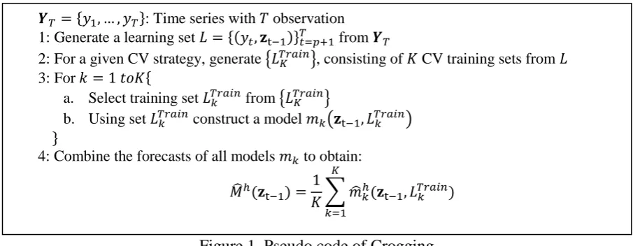
Figure 1. Pseudo code of Crogging
Figure 1 is a pseudo code of the crogging framework for combining forecasts. Given a
time series we generate a set of input/output pairs as described in Section 3. Having selected
a cross-validation strategy, described later, we generate a set of 𝐾 training sets each used to
estimate a single forecast model. Each training set is the result of a split of the learning set
into a training dataset for estimating the forecast model, and a validation dataset for early stop
training to reduce overfitting. Note that a separate test set will be used which will be the
holdout sample on which out-of-sample accuracy is evaluated. The aggregate forecast is
taken as the simple average of all 𝐾 forecasts as follows:
𝑀̂ℎ(𝐳
t−1) = 1
𝐾∑ 𝑚̂𝑘 ℎ(𝐳
t−1, 𝐿𝑇𝑟𝑎𝑖𝑛𝑘 ) 𝐾
𝑘=1
(4)
}
𝑀̂ℎ(𝐳 t−1) =
1
𝐾∑ 𝑚̂𝑘ℎ(𝐳t−1, 𝐿𝑇𝑟𝑎𝑖𝑛𝑘 ) 𝐾
𝑘=1 𝒀𝑇 = {𝑦1, … , 𝑦𝑇}: Time series with 𝑇 observation 1: Generate a learning set 𝐿 = {(𝑦𝑡, 𝐳t−1)}𝑡=𝑝+1𝑇 from 𝒀𝑇
2: For a given CV strategy, generate {𝐿𝑇𝑟𝑎𝑖𝑛𝐾 }, consisting of 𝐾 CV training sets from 𝐿
3: For 𝑘 = 1 𝑡𝑜𝐾{
a. Select training set 𝐿𝑇𝑟𝑎𝑖𝑛𝑘 from {𝐿𝐾𝑇𝑟𝑎𝑖𝑛}
b. Using set 𝐿𝑇𝑟𝑎𝑖𝑛𝑘 construct a model 𝑚𝑘(𝐳t−1, 𝐿𝑇𝑟𝑎𝑖𝑛𝑘 )
10
where 𝐿𝑇𝑟𝑎𝑖𝑛𝑘 is the 𝑘𝑡ℎ training dataset and 𝑚̂𝑘(𝐳t−1, 𝐿𝑇𝑟𝑎𝑖𝑛𝑘 ) is the model estimated using that
dataset.
3.2.1. k-fold crogging
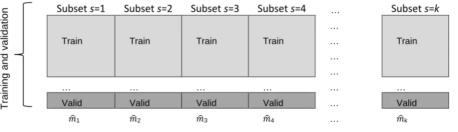
Within the general setting provided in Section 3.2, we define a k-fold cross-validation
over the learning set 𝐿, as a division or splitting of 𝐿 into k none-overlapping and mutually
exclusive subsamples or folds of approximately equal size, with 𝑘 ≤ 𝐷. The procedure for
doing this is depicted in Figure 2.
Subset s=1 Subset s=2 Subset s=3 Subset s=4 … Subset s=k
Train Train Train Train
…
Train …
… …
… … … …
Valid Valid Valid Valid … Valid
[image:11.595.86.538.291.421.2]𝑚̂1 𝑚̂2 𝑚̂3 𝑚̂4 … 𝑚̂k
Figure 2. Example of k-fold cross-validation
Observations are drawn at random, but unlike in a bootstrap sample, without replacement. In
each round 𝑘, we obtain a dataset 𝐿𝑇𝑟𝑎𝑖𝑛𝑘 comprised of k-1 subsamples, and use this to
estimate the parameters of a forecast model 𝑚̂𝑘(𝐳t−1, 𝐿𝑇𝑟𝑎𝑖𝑛𝑘 ). This process is repeated k
-times, so that each of the 𝑘 subsamples are used exactly k-1 times as training data and once as
validation data (see Figure 2). The combined forecast is then aggregated using Eq. (4),
resulting in a combined forecast based on the given 𝑘-fold cross-validation strategy. In this
case k the number of subset folds is also equal to 𝐾 the sampling size. Where a single model
is estimated on each sample then 𝐾 is also the combination size.
Typically, k-fold cross-validation can apply a different number of folds with different
properties depending on the value of k. For k= 2 we obtain a split of the learning set into 2
subsamples of approximately equal size, the first used for training and the second for
T
rai
ni
ng
an
d v
a
lida
ti
o
11
validation, and visa versa. The 10-fold validation is the most commonly applied
cross-validation strategy having obtained good results in practice (Kohavi 1995; Hu et al. 1999),
and with some theoretical evidence (Bengio and Grandvalet 2004). The learning set is split
into 10 approximately equal subsamples, training on a dataset of 9 subsamples, with one
subsample for validation. Another common strategy is the leave-one-out (LOO)
cross-validation, training on 𝑁 − 1 subsamples, with each subsample containing a single
observation for validation. The general form of k-fold will be evaluated for different sample
sizes including 2-fold and 10-fold, while the leave-one-out method will serve as a benchmark
for our evaluation on real data.
An overall advantage of 𝑘-fold cross-validation, is that each observation is used both
for training and validation, with equal weight of 𝑘 − 1 during training, and once for
validation. A potential drawback is that 𝑘 controls the trade-off between data available to
train each model for a valid in-sample estimation, and data available for validation to
estimate out-of-sample accuracy and control overfitting, LOO cross-validation being the
extreme case.
3.2.2. Monte Carlo crogging
Each method suffers from one of more limitations as described previously. For
example, k-fold and leave-one-out cross-validation are known to be asymptotically
inconsistent (Efron 1983; Efron and Tibshirani 1986; Shao 1993; Stone 1977; Shao 1997). In
the context of forecasting combination this means that both approaches may lead to
overfitting, performing well in-sample but poorly out-of-sample. While k-fold cross
validation has been found in some cases to perform better than leave-one-out (Breiman 1984;
Burman 1989; Zhang 1993), it can suffer from unacceptably high variance leading to
12
In contrast the Monte Carlo cross-validation strategy (Picard and Cook 1984),
sometimes referred to as repeated random subsampling validation is known to be
assymptotically consistent, and less prone to overfitting (Shao 1993). The reduced overfitting
is a consequence of the decoupling of the validation set and sampling size which enhances
the potential impact of validation and therefore reduces the risk of overfitting. A larger
validation set may however hinder the accurate estimate of the prediction error, due to the
smaller training set, a trade-off between model parameter estimation and validation. Where
predictive accuracy is the goal as is the case in forecasting, it was shown that Monte Carlo
cross-validation provides a larger probability than Leave-one-out cross-validaton of selecting
the model with best prediction ability (Shao 1993).
Monte Carlo cross-validation works by randomly splitting the learning set 𝐾 times,
each time randomly drawing without replacement 𝐽 pairs to form the training set 𝐿𝑇𝑟𝑎𝑖𝑛, and
using the remaining 𝐷 − 𝐽 pairs to form 𝐿𝑉𝑎𝑙𝑖𝑑. In this regard Monte Carlo cross-validation is
similar to Bagging where ‘out-of-bag’ observations are used as validation set, the main
difference being that with the later sampling is performed with replacement. On each round
of Monte Carlo cross-validation, a forecast model is estimated, and the aggregate of all 𝐾
forecasts is obtained using Eq. (4). Although the training and validation datasets are mutually
exclusive for each round of Monte Carlo cross-validation as in k-fold cross-validation,
between rounds an observation may appear in the training or validation dataset any number of
times depending on the independent random sampling between rounds, as in bagging. This is
because on each round, sampling is performed without replacement (therefore the same
observation does not appear in both the training and validation sets), whereas between
rounds, sampling is performed with replacement similar to the bootstrap sampling in each
round of bagging. Another potential advantage over 𝑘-fold cross-validation is in the number
cross-13
validation, Monte Carlo cross-validation is able to create forecast combinations (training sets)
much larger than k, theoretically infinite, albeit at the expense of determining another
metaparameter of the number of Monte Carlo samples. This study provides the first empirical
results on the application of Monte Carlo cross-validation for forecast combination.
3.2.3. Holdout cross-validation
A special case of k-fold and Monte Carlo cross-validation widely is the holdout
method which results in a single split of the learning set into a training and validation set
(Bengio and Grandvalet 2004). With observations of a time series often split sequentially,
with the validation data containing the most recent observations consecutively, holdout
cross-validation is more similar to k-fold than Monte Carlo cross-validation, although
non-sequential splitting as in Monte Carlo cross-validation is also feasible. One criticism of the
holdout method is that it does not account for the variance with respect to the training set
(Dietterich 1998). Research on the optimal number of observations to include in either dataset
is also inconclusive, with heuristic rule of thumb, 70%:30% split into training and validation
typically applied in practice. As there is only a single data split, the strategy cannot be applied
directly for forecast aggregation. However due to its simplicity, the holdout method is widely
applied in model selection (Arlot and Celisse 2010), and common in neural network training
with early stopping to prevent overfitting. In this study we will use the holdout method as a
benchmark for 1) forecast model selection referring to it as Holdoutselect and model averaging
referring to it as Holdoutavg. We also evaluate model averaging without the use of a
validation set. Each network is trained on the entire learning set and allowed to overfit, with
the forecasts subsequently averaged to obtain the combined forecast. We refer to this method
14
3.3. Theoretical performance of crogging
In this section we apply the ambiguity decomposition of Brown et al. (2005) in
assessing the predictive performance of crogging. We show that for a given observation, the
squared error of the combined 1-step-ahead forecast is no more than the average squared
error of the individual forecasts. This means that with no guarantee of selecting a forecast
with error lower than the combined forecast, we are at least guaranteeed of having
1-step-ahead performance better on average than a forecast selected at random.
For crogging, we write the squared error (SE) of the combined forecast given by Eq.
(2) for the 1-step-ahead forecast as SE = (𝑀̂(𝐳𝑡−1) − 𝑦𝑡)2. In comparison the average
squared error of the constituent forecast models can be expressed as:
∑1
𝐾(𝑚̂𝑘(𝐳𝑡−1) − 𝑦𝑡)2 𝑘
= ∑1
𝐾(𝑚̂𝑘(𝐳𝑡−1) − 𝑀̂(𝐳𝑡−1) + 𝑀̂(𝐳𝑡−1) − 𝑦𝑡) 2
𝑘 = ∑1
𝐾[(𝑚̂𝑘(𝐳𝑡−1) − 𝑀̂(𝐳𝑡−1)) 2
+ (𝑀̂(𝐳𝑡−1) − 𝑦𝑡)2 𝑘
+ 2 (𝑚̂𝑘(𝐳𝑡−1) − 𝑀̂(𝐳𝑡−1)) (𝑀̂(𝐳𝑡−1) − 𝑦𝑡)]
Using ∑ 1
𝐾 = 1
𝑘 and 𝑀̂(𝐳𝑡−1) = ∑𝑘𝐾1𝑚̂𝑘(𝐳𝑡−1)cross-terms disappear and we get:
∑1
𝐾(𝑚̂𝑘(𝐳𝑡−1) − 𝑦𝑡)2 𝑘
= ∑1
𝐾(𝑚̂𝑘(𝐳𝑡−1) − 𝑀̂(𝐳𝑡−1)) 2
+ (𝑀̂(𝐳𝑡−1) − 𝑦𝑡) 2
𝑘
= ∑𝑘𝐾1(𝑚̂𝑘(𝐳𝑡−1) − 𝑀̂(𝐳𝑡−1))2+ SE
Rearranging we obtain:
SEℎ = ∑1
𝐾(𝑚̂𝑘(𝐳𝑡−1) − 𝑦𝑡)2 𝑘
− ∑1
𝐾(𝑚̂𝑘(𝐳𝑡−1) − 𝑀̂(𝐳𝑡−1)) 2
𝑘
Observe that the second term ∑ 1
𝐾(𝑚̂𝑘(𝐳𝑡−1) −𝑀̂(𝐳𝑡−1)) 2
𝑘 , the ambiguity term, is always
positive and therefore reduces the first term, the average error of the individual forecasts. The
larger the ambiguity term or equivalently the variance among the individual forecasts, the
15
individual 1-step-ahead forecasts 𝑚̂𝑘(𝐳𝑡−1) generated based on the cross-validation replicates
of 𝐿, the larger the potential improvement from crogging. Conversely if the 1-step-ahead
forecasts are very similar, the ambiguity will be small and the error of the combined forecast
will be close to the average error of the individual forecasts.
While an h-step-ahead analysis is beyond the scope of this study, it has been shown
that the 1-step-ahead bias and variance affects the h-step-ahead bias and variance for the
recursive multi-step forecasting strategy (Taieb and Atiya 2015). In particular they find that
for complex model’s such as neural networks (NNs), both the bias and variance tend to
increase with the forecast horizon, in particular due to the large variance. We hypothesize that
as cross-validation involves systematic resampling and training on the complete learning set,
it will be effective at increasing ambiguity, while not adversely affecting the bias of the
individual forecasts, and as a consequence improve the accuracy of the combined forecast. In
the next section we investigate the performance of crogging from a bias and variance
perpective estimated via Monte Carlo simulation. Future research should pursue a more
detailed theoretical analysis of the h-step-ahead bias and variance in assessing the impact of
each method.
4.
Bias and variance decomposition of Crogging
4.1. Overview
In order to assess the efficacy of k-fold and Monte Carlo crogging algorithms, we
carry out a Monte Carlo simulation study to investigate the impact of the size of the forecast
combination, and the time series length on the bias and variance of the prediction. With
forecast performance measured by MSE, we decompose the MSE of the combined forecast
into its bias and variance components (Geman, Bienenstock, and Doursat 1992), using the
16
The results are compared to bagging in order to allow a comparison to its better understood
properties.
We adopt the same terminology as in Taieb and Hyndman (2014) and assuming that
the process defined in Eq. (1) is stationary, we obtain the bias and variance components of the
mean squared error of h-step-ahead combined forecast MSEℎ as follows:
MSEℎ= 𝔼𝐱t[(𝑦𝑡+ℎ− 𝑀̂ℎ(𝐳
𝑡−1))2| 𝐱t]
= 𝔼𝐱t,ε[(𝑦𝑡+ℎ− 𝜇𝑡+ℎ|𝑡)2| 𝐱t] Noise
+𝔼𝐱t[(𝜇𝑡+ℎ|𝑡− 𝑀ℎ(𝐳𝑡−1)) 2
] Squared Bias
+𝔼𝐱t,𝒀𝑇[(𝑀̂ℎ(𝐳
𝑡−1) − 𝑀ℎ(𝐳𝑡−1))2| 𝐱t] Variance
(5)
where 𝑀ℎ(𝐳𝑡−1) = 𝔼[𝑀̂ℎ(𝐳𝑡−1)], 𝑀̂ℎ(𝐳𝑡−1) is the combined ℎ-step-ahead forecast for a
given combination strategy, and𝔼𝑥 and 𝔼[∙|𝑥] represent the expectation over 𝑥, and the
expectation conditional on 𝑥, respectively. The resulting decomposition gives us a measure of
the noise, the squared bias, and an estimate of the variance of the combination method.
4.2. Experimental design and data
For each combination strategy we estimate Eq.(5) via simulation considering a linear
AR(6) and a nonlinear Smooth Transition Autoregressive (STAR) data generating process
(DGP) also used by Ben Taieb and Hyndman (2014). The linear AR(6) process is given by:
𝑦𝑡= 1.32𝑦𝑡−1− 0.52𝑦𝑡−2− 0.16𝑦𝑡−3+ 0.18𝑦𝑡−4− 0.26𝑦𝑡−5+
0.19𝑦𝑡−6+ 𝜀𝑡 .
(6)
where 𝜀𝑡~NID(0, 1). The STAR process has been used in several other studies (e.g.
Terasvirta and Anderson 1992; Berardi and Zhang 2003) for understanding nonlinearities in
17
𝑦𝑡 = 0.3𝑦𝑡−1+ 0.6𝑦𝑡−2+ (0.1 − 0.9𝑦𝑡−1+ 0.8𝑦𝑡−2)[1 + 𝑒(−10𝑦𝑡−1)]
−1
+ 𝜀𝑡 (7)
where𝜀𝑡~NID(0, 𝜎2) and the error variance set to 𝜎2 = 0.052.
We generate time series of length 𝑇 ∈ {50, 400} in order to assess the impact of time
series length on the bias and variance of each strategy. The number of forecasts included in
the final combination is deemed critical to its performance (de Menezes, Bunn, and Taylor
2000). This is determined by the number of training sets or sampling size of each strategy
which in turn determines the number of models which can be estimated. The sampling sizes
evaluated are taken from the set {2, 5, 10,15, 20, 30}. For k-fold cross-validation this sample
size is also equalivalent to the number of folds 𝑘, while for Monte Carlo crogging and
bagging this is equivalent to the number of random splits and the number of bootstraps
respectively. If for every sample bootstrap or cross-validation a single model is estimated,
then the sampling size is also equal to the forecast combination size 𝐾.
4.3. Estimation
We generate for each DGP, a set of 1000 independent time series 𝑆𝑖 = {𝑦1, … , 𝑦𝑇} on
which to train and estimate model parameters. To give an objective measure of the bias and
variance components, we generate an independent time series from the same DGP serving as
a test set. From this independent series, we obtain a set of 2000 input/output pairs
{(𝐲𝑗, 𝐳𝑗)}𝑗=12000 where 𝐳𝑗 is the lagged vectors of inputs, and the vector 𝐲𝑗 is the next 𝐻
consecutive observations representing the lead time to be forecasted, in our case set to 10.
The MSE is then calculated as follows:
MSEℎ = 1
1000 × 2000 ∑ ∑ (𝐲𝑗ℎ− 𝑀̂𝑆𝑖
ℎ(𝐳 𝑗))
𝟐 2000
𝑗=1 1000
𝑖=1
18
Noiseℎ = 1
2000∑ (𝐲𝑗ℎ− 𝔼[𝐲𝑗ℎ | 𝐳𝑗])
𝟐 2000
𝑗=1
Biasℎ2 = 1
2000 ∑ (𝔼[𝐲𝑗ℎ | 𝐳𝑗] − 𝑀̅(𝐳𝑗))
𝟐 2000
𝑗=1
Varianceℎ = 1
1000 × 2000 ∑ ∑ (𝑀̂𝑆𝑖
ℎ(𝐳
𝑗) − 𝑀̅(𝐳𝑗))
𝟐 2000
𝑗=1 1000
𝑖=1
where 𝑀̅(𝐳𝑗) =10001 ∑ 𝑀̂𝑆𝑖
ℎ(𝐳 𝑗) 1000
𝑗=1 is an estimate of 𝑀ℎ(𝐳𝑗) and 𝑀̂𝑆𝑖
ℎ(𝐱
𝑗) is the combined
forecast produced using dataset 𝑆𝑖. The variable 𝐲𝑗ℎ is the ℎth element of the vector 𝐲𝑗,
representing the h-step-ahead forecast. Throughout this study, forecasts are produced using
the recursive strategy due to its simplicty, intuition, widespread use in research and practice,
and reduced computational load. This is in contrast to the direct strategy which although
being immune to propagation of forecast errors, would require a different model combination
for each forecast horizon, and becoming rather intensive computationally (Taieb et al. 2012).
The conditional mean 𝔼[𝐲𝑗ℎ | 𝐳𝑗] for the linear process is calculated analytically. In the case
of the nonlinear process, we average over a large number of possible values for each future
time point of the series using simulation. In all cases we use a Multilayer Perceptron (MLP),
a feedforward neural network capable of approximating linear and nonlinear data generating
processes. We employ the same MLP setup as described in Section 5.3 with 𝑝 = 6. For
Monte Carlo crogging we set the training-validation split to 70% - 30%.
4.4. Experimental Results
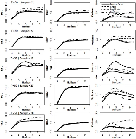
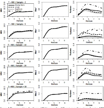
Results of the bias-variance decomposition including the MSE (first column), the bias
(second column) and the variance (third column) for the linear and nonlinear DGP are shown
in Figure 3 and Figure 4 respectively, for short series having length 𝑇 = 50. The MSE
provides a measure of the forecast error of the different combination approaches, Monte
19
examination of the strengths of the competing approaches across sampling sizes. For both
DGPs, we can see that the largest of the three components is the bias which, as the number of
samples and forecast horizon increases, is nearly two to three times as large as the variance.
This suggests that the neural network base model structure with 2 hidden nodes and 𝑝 = 6
autoregressive inputs, may not be sufficient to approximate the underlying DGP in the
presence of the given noise level. Nevertheless, this scenario reflects the core challenge in
real forecasting problems, where often the ’true‘ model stucture is not known in advance of
model fitting and the data has significant levels of noise relative to the signal in the data. In
contrast, where the model structure is known, then the DGP can trivally be estimated to high
accuracy using NNs.
Considering the differences between the methods, Figure 3 shows that for the linear
process, BagFoob and k-fold both have the highest variance while Monte Carlo consistently
has the smallest variance on average across all horizons. This improvement has however not
induced a large increase in bias. On the contrary, the bias of Monte Carlo is generally equal
to, if not less than other methods, and consequently the forecasts for Monte Carlo outperform
20
Figure 3.Decomposition for linear AR(6) processfor different sampling sizes showing MSE, bias and variance for time series length T=50 and forecast horizon of10.
BagMoob is often nearly as good as Monte Carlo particularly at small sampling sizes
where it has similar performance in terms of variance and on average across horizons
outperforms k-fold and BagFoob. As sampling size increases up to 30 samples, this relative
performance in terms of variance is still present; however the difference between methods in
terms of bias is smaller. The difference in performance among methods appear to come
21
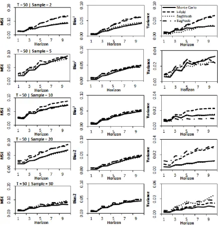
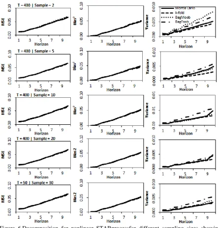
Figure 4.Decomposition for nonlinear STAR processfor different sampling sizes showing MSE, bias and variance for time series length T=50 and forecast horizon of 10.
Results of the nonlinear DGP shown in Figure 4 are similar to those obtained on the
linear DGP, with Monte Carlo on average having the lowest variance and best forecasts in
terms of MSE across sampling sizes. This is followed closely by BagMoob which at sampling
sizes less than 20 performs similarly. As sample size increases, both BagFoob and k-fold
improve in performance however no consistent difference is noted between the two methods.
However with the exception of sampling size 10 where BagFoob performs well on variance,
[image:22.595.75.514.69.523.2]22
Figure 5.Decomposition for linear AR(6)processfor different sampling sizes showing MSE, bias and variance for time series length T=400 and forecast horizon of 10.
The evidence therefore indicates that Monte Carlo is best at reducing variance while
not adversely increasing the bias of the combined forecast, and that BagMoob is on average
always better than BagFoob. In fact, for both the linear and nonlinear DGP and across all
sampling sizes, Monte Carlo always produces a forecast having smaller bias than k-fold and
BagFoob, and which consequently leads to improved accuracy overall. On linear time series, k
-fold on average outperforms BagFoob across all sampling sizes and forecast horizons while for
[image:23.595.74.515.69.529.2]23
Figure 6.Decomposition for nonlinear STARprocessfor different sampling sizes showing MSE, bias and variance for time series length T=400 and forecast horizon of 10.
This is possibly due to the sampling scheme of cross-validation and BagMoob which uses a set
of ‘out of bag’ observations which guarantees that all observations in the learning set are used
for training. In contrast for BagFoob observations in the validation set are never used for
training. Additionally for short time series, linear or nonlinear Monte Carlo which like
bagging involves some random sampling appears to be much more effective at reducing
[image:24.595.73.517.68.533.2]24
These results hold, if not much clearer, for the longer time series having 400
observations. For both the linear and nonlinear DGP, total forecast error is reduced with the
significant reductions coming from the variance component. In fact the bias for all four
methods, which is now considerably larger than the variance, is nearly equal across all
sample sizes for all methods, while the variance of Monte Carlo and BagMoob is on average
always lower than k-fold and BagFoob. Though small this results in a consistent improvement
in MSE from using Monte Carlo over k-fold crogging, and BagMoob compared to BagFoob.
5.
Empirical Evaluation Experiment
5.1. Design of combination methods
In this real-world experiment, we compare the forecasting accuracy of 𝑘-fold and
Monte Carlo crogging to bagging, conventional neural network model averaging over
multiple initialisations, and individual neural network model selection. One objective of this
study is to determine which, if any, of the combination strategies is best for forecast
combination, and under what conditions of sample size, and time series length. For each
method we use the same number of samples to train, using the identical neural network set up
and weight initialisation, to ensure that any differences in the forecast accuracy are
attributable directly to the method of choice, allowing a fair and robust comparison. We train
a total of 50 networks, each with different random starting weights to account for error
variance from local minima in the network training.
For 𝑘-fold cross-validation we evaluate 𝑘 = 2, 5, 10, 15, 20, 25 and 30producing a
corresponding number of data splits for training. For example, in the case of 2-fold
cross-validation, we obtain 2 splits of the learning set and for each split, train 50 similarly
initialized networks producing altogether 100 forecasts. Similarly when k=10 we have
25
direct comparison with k-fold crogging, we again create Monte Carlo cross-validation
samples of size 2, 5, 10, 15, 20, 25 and 30 using the same randomly initialized networks. We
implement BagFoob, and BagMoob in the same manner allowing a fair and robust comparison.
5.2. NN3 competition Dataset
To empirically evaluate the performance of each method, we utilise the 111 time
series from the NN3 competition dataset consisting of a representative set of long and short,
seasonal and non-seasonal monthly time series drawn from a homogenous population of
empirical business series (Crone, Hibon, and Nikolopoulos 2011). The time series contain
between 68 and 144 observations. The reduced dataset contains a mixture of all time series
types of which three are characterised as difficult to forecast, 4 as seasonal and the remaining
7 as non-seasonal containing also outliers and structural breaks. A summary of the
characteristics of the time series is provided in Table 1.
Table 1: Summary description of NN3 competition time series dataset
Complete Dataset
Reduced Dataset
Short Long Normal Difficult SUM
Non-Seasonal 25
(NS)
25 (NL)
4 (NN)
3
(ND) 57
Seasonal 25
(SS)
25 (SL)
4
(SN) - 54
SUM 50 50 8 3 111
For each method using a fixed validation set the number of observations is set to 14 to allow
for estimating of monthly seasonlity in the shortest possible series being 68 observations and
with 18 needed for the test dataset. However these observations are not always fixed as with
Monte Carlo crogging and BagMoob which sample different obervations for the validation set.
5.3. Design of benchmark Algorithms
26
Noholdoutavg and BagNoob we use the same identically initialized 50 MLPs as with the
principal combination methods. In the case of Holdoutselect or individual model selection we
select the network from the 50 differently initialized MLPs having the smallest MSE on the
fixed size validation set. For Holdoutavg we average over the predictions of these same
networks while for the Noholdoutavg method we average over each network this time trained
without a validation set. This approach of averaging over multiple weight initializations of
the same neural network architecuture is also known as neural network model averaging
(Hansen and Salamon 1990). Both model averaging and model selection are two established
methods of building neural network models for time series forecasting (Zhang and Berardi
2001; Naftaly, Intrator, and Horn 1997) both based on the Holdout method. Consequently
they provide strong benchmarks for this study, and allow investigating the benefits of
cross-validation versus ordinary cross-validation (holdout). In the case of BagNoob we train each of the 50
networks on a bootstrap sample but unlike BagFoob and BagMoob no validation set is used
therefore the entire learning set is bootstrapped.
5.4. MLP setup
For the implementation of crogging, bagging, neural network averaging and selection
we use the same base learner of a univariate Multilayer Perceptron (MLP). MLPs are well
researched, and their ability to approximate and generalize well any functional relationship to
an arbitrary degree of accuracy has been proven (Hornik, Stinchcombe, and White 1989;
Hornik 1991). In particular, they have been shown empirically to be able to forecast linear
and nonlinear time series of different forms (Zhang, Patuwo, and Hu 1998). The functional
form of these networks is given by:
𝑚̂(𝐳𝑡) = 𝛽0+ ∑ 𝛽ℎ𝑔 (𝛾0𝑖+ ∑ 𝛾ℎ𝑖
𝐼
𝑖=0
𝑝𝑖)
𝐻
𝑘=1
27
with 𝐼 = 13, inputs 𝑝𝑖, connected to each of 𝐻 hidden nodes in a single hidden layer using
the hyperbolic tangent transfer function, and a single output node with an identity function.
This is sufficient to model monthly seasonality stochastically in addition to trends effectively
combining an 𝐴𝑅(12) and 𝐴𝑅(1) process. To evaluate the impact of model complexity we
consider neural networks having hidden nodes 𝐻 = 1, … ,5. The architecture of the MLP is
otherwise exactly the same allowing a fair assessment of the impact of the number of hidden
nodes on performance of each combination method. Each time series is modelled directly
without prior differencing or further data transformation to estimate level, seasonality, and
potential trend directly in the network weights and the bias terms. Additionally all time series
are linearly scaled into the interval of [-0.5, 0.5] to allow headroom for possible
non-stationarity prior to training. We produce multistep forecasts using an iterative prediction,
recursively generating one-step-ahead forecasts.
For parameter estimation the Levenberg-Marquardt algorithm (Hagan, Demuth, and
Beale 1996) is used to minimise the MSEloss function up to a maximum of 1000 epochs. The
algorithm requires setting a scalar 𝜇𝐿𝑀 and its increase and decrease steps, using 𝜇𝐿𝑀 =
10−3, with an increase factor of 𝜇
𝑖𝑛𝑐 = 10 and a decrease factor of 𝜇𝑑𝑒𝑐 = 10−1. All
network training employ an early stopping criterion in order to avoid overfitting. This means
that we track the MSE on the training and the validation set, and halt the training process and
retain the network weights with the lowest error on the validation data after the error has not
decrease for more than 50 epochs, or if 𝜇𝐿𝑀 exceeds 𝜇𝑚𝑎𝑥 = 1010. For each new forecast
model, we randomly initialize the starting weights for each MLP allowing for different
solutions of the network to be achieved, taking care to ensure that the same starting weights
are used for each method. This is in addition to the randomness introduced by the k-fold,
28
5.5. Evaluation
The forecast horizon for all methods is set to 12 months using a holdout sample of 1
to 18 months in the future, and a rolling origin evaluation to assess forecasting accuracy and
performance (Tashman 2000). The size of the validation set during training depends on the
method used, leaving the remaining observations for training. Where a fixed size validation
set is used then it is set to 14 observations as explained in Section 5.2. In comparing results to
that of the NN3 competitors (benchmarking), the forecast horizon will later be extended to 18
steps ahead forecasting from a fixed origin, as required by competition guidelines. We
calculate the mean absolute scaled error (MASE) and the symmetric mean absolute error
(SMAPE) for all methods in assessing forecast accuracy and performance. For a given actual
𝑋𝑡, and forecast 𝐹𝑡 the SMAPE (Chen and Yang 2004) provides a scale independent measure
that can be used to compare accuracy across time series . It is calculated as follows:
𝑆𝑀𝐴𝑃𝐸 = 1
𝑁∑ (
|𝑋𝑡− 𝐹𝑡|
(|𝑋𝑡| + |𝐹𝑡|) 2⁄ )
𝑁
𝑡=1
(9)
where 𝑁 is the number of observations in the training set and 𝐻 is the number of values being
forecasted in the out-of-sample test set.
Hyndman and Koehler (2006) propose the use of the MASE as it is less sensitive to
outliers and more easily interpretable than other scaled error measures. The MASE is defined
as follows:
𝑀𝐴𝑆𝐸 = 1
𝐻∑ (
|𝑋𝑡− 𝐹𝑡|
(𝑁 − 1)−1∑ |𝑋
𝑖− 𝑋𝑖−1| 𝑁
𝑖=2
)
𝐻
ℎ=1
(10)
To assess whether observed differences in MASE and SMAPE are statistically significant,
the nonparametric Friedman test (Milton 1940, 1937) which requires no assumption about the
distribution of forecast errors, and the post-hoc Nemenyi test (Nemenyi 1962) are employed.
29
statistically different from the rest outputting a p-value. The Nemenyi test is based on the
minimum distance between methods being compared such that methods are considered to be
statistically different if the difference between the ranks of methods compared is larger than
this ‘critical’ distance.
6.
Results
6.1. Overall performance
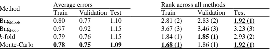
The overall results on bagging and crogging are provided in Table 2. For ease of
presentation, results are shown using only MASE as no statistically significant differences are
noted between results based on MASE and SMAPE. It gives the results for the NN3
competition data for training, validation and test dataset, showing MASE averaged across all
time series, sampling sizes and number of hidden nodes. Ranks based on the Nemenyi test
are also shown for all datasets. Methods having no statistically significant difference in
performance share the same ranking should in brackets. The method with the lowest average
error is highlighted in bold, while those with the best model ranking is highlight in bold and
[image:30.595.73.525.542.624.2]underlined where the average ranking is best.
Table 2. Average errors and and rank of errors on the complete dataset by method. Ranking of errors is based on the Nemenyi Test.
Method Average errors Rank across all methods
Train Validation Test Train Validation Test
BagMoob 0.80 0.77 1.10 2.81 (2) 2.83 (2) 1.92 (1)
BagFoob 0.97 0.92 1.15 3.67 (3) 3.46 (3) 3.23 (3)
k-fold 0.79 0.76 1.15 1.84 (1) 1.85 (1) 2.93 (2)
Monte-Carlo 0.78 0.75 1.09 1.68 (1) 1.86 (1) 1.92 (1)
The best method in each column is in boldface. The method with the best ranking is underlined. Methods with no statistically significant differences at the 0.05 level of significance share the same model ranking shown in brackets.
Across all series, Monte Carlo crogging, Monte-Carlo, has the lowest average MASE
on the test set, as well as the best average ranking although results indicate no statistically
significant difference in performance over bagging with moving ‘out-of-bag’, BagMoob. Both
30
bagging with fixed ‘out-of-bag’, BagFoob. k-fold crogging outperforms and is statistically
better than BagFoob suggesting that there are benefits in acurracy from having diffferent
samples in the validation sets. For all methods out-of-sample results are consistent with those
obtained in-sample on the training and validation datasets in terms of average errors, however
results on rankings suggest that Monte-Carlo is more consistent. In-sample it ranks
statistically better than BagMoob on training and validation datasets, and out-of-sample is just
as good if not better on average error. This suggests that crogging is likely to be more robust
to overfitting and issues of method selection particularly when selection is based on
in-sample model fit. In the next section we consider performance based on the properties of the
tiem series data.
6.2. Data properties
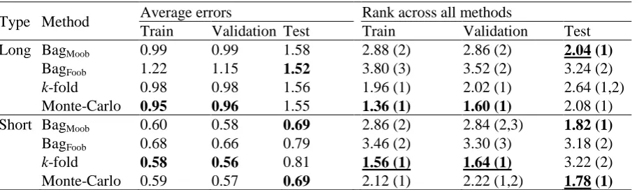
Table 3 shows the results of average MASE and ranking for long and short series
across sample size and number of hidden nodes for all four methods. Results show no
statistically significant differnces between Monte-Carlo and BagMoob. While BagMoob ranks
best on the test set with an average rank of 2.04 for long series, Monte-Carlo is best on short
series having an average ranking of 1.78. In-sample k-fold performs well ranked best on
training and validation dataset for short time series. However unlike Monte-Carlo which also
performs well on the test set, k-fold does not show similar performance out-of-sample
indicating evidence of overfitting as previously discussed. The effect of overfitting seems
reduced on long series where it is ranked joint first with no statistically significant difference
in performance compared to Monte-Carlo and BagMoob. BagFoob is always outranked by
Monte-Carlo and BagMoob across all datasets although it does well in terms of average errors
on test set for long series. This difference between ranks of errors and average errors suggests
that there are several difficult time series, particularly affecting the less robust average of
31
Table 3. Average errors and and rank of errors on the test dataset by method and time series length. Ranking of errors is based on the Nemenyi Test.
Type Method Average errors Rank across all methods
Train Validation Test Train Validation Test Long BagMoob 0.99 0.99 1.58 2.88 (2) 2.86 (2) 2.04 (1)
BagFoob 1.22 1.15 1.52 3.80 (3) 3.52 (2) 3.24 (2)
k-fold 0.98 0.98 1.56 1.96 (1) 2.02 (1) 2.64 (1,2)
Monte-Carlo 0.95 0.96 1.55 1.36 (1) 1.60 (1) 2.08 (1) Short BagMoob 0.60 0.58 0.69 2.86 (2) 2.84 (2,3) 1.82 (1)
BagFoob 0.68 0.66 0.79 3.46 (2) 3.30 (3) 3.18 (2)
k-fold 0.58 0.56 0.81 1.56 (1) 1.64 (1) 3.22 (2)
Monte-Carlo 0.59 0.57 0.69 2.12 (1) 2.22 (1,2) 1.78 (1)
The best method in each column is in boldface. The method with the best ranking is underlined. Methods with no statistically significant differences at the 0.05 level of significance share the same model ranking shown in brackets.
The order of rankings is similar when considering seasonal and non-seasonal data as
shown in
Table 4. Again no statistically significant difference is noted in the ranking of
Monte-Carlo and BagMoob although Monte-Carlo gives the best ranking on seasonal time seris while
on non-seasonal BagMoob is ranked best. While both methods show no staistically significant
differnces on the test set, on the training and validation datset, Monte-Carlo is always
statistically better than BagMoob. This may potentially be explained by the structured nature of
the sampling in Monte Carlo crogging, in that while observations are drawn at random, it is
done without replacement ensuring that observations only appear in the trainining set once
and therefore more distrinct observations can be sampled. In contrast, when BagMoob is used,
observations in the training set may repeat offfering fewer distinct obsevations on which to
train. The performance of Monte-Carlo and BagMoob would suggest that the feature of the
randam sampling across both the training and validation set are important; coventional
bagging which in contrasts involves random sampling but only of the training set appears to
be inferior
32
Type MASE Average errors Rank across all methods
Method Train Validation Test Train Validation Test Non-seasonal BagMoob 0.98 0.99 1.56 2.74 (2) 2.76 (2) 1.96 (1)
BagFoob 1.21 1.15 1.52 3.56 (3) 3.40 (2) 3.20 (2)
k-fold 0.98 0.98 1.56 1.86 (1) 1.76 (1) 2.86 (2) Monte-Carlo 0.96 0.97 1.53 1.84 (1) 2.08 (1) 1.98 (1) Seasonal BagMoob 0.61 0.58 0.71 3.00 (2) 2.94 (2) 1.90 (1)
BagFoob 0.69 0.67 0.80 3.70 (3) 3.42 (2) 3.22 (2)
k-fold 0.58 0.56 0.80 1.66 (1) 1.90 (1) 3.00 (2) Monte-Carlo 0.59 0.57 0.71 1.64 (1) 1.74 (1) 1.88 (1)
The best method in each column is in boldface. The method with the best ranking is underlined. Methods with no statistically significant differences at the 0.05 level of significance share the same model ranking shown in brackets.
While the above provides a good overview of the performance of the four methods, it
is does not account for the potential difference in forecasting accuracy of each method as
sampling size and number of time series observations change, discussed next.
6.3. Sampling size
We investigate how the choice of sampling size and the interaction with time series
length affects forecasting accuracy. Recall that for k-fold cross-validation the number of
training sets is equivalent to the number of folds 𝑘, while for Monte Carlo crogging and
bagging this is equivalent to the number of random splits and the number of bootstraps
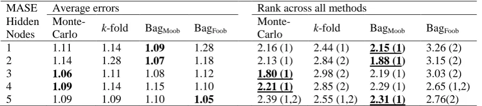
respectively. Table 5 shows the results for the average MASE and ranking by time series
length and sample size. The most accurate method on average for each sampling size (by
row) is highlighted in bold, while the most accurate method across sampling sizes is
underlined, for both long and short series. Ranking is done by method for each sample size.
Results of average error indicate that Monte-Carlo and BagMoob rank best on short
series for nearly all sampling sizes. In contrast both methods perform comparatively poorly
on long time series and are outperformed by BagFoob across nearly all sample sizes. Results
based on rankings are somewhat different and show Monte-Carlo to be robust across time
33
Table 5. Average errors and and rank of errors on test dataset by method and sampling size. Ranking of errors is based on the Nemenyi Test.
Type Size
Average errors Rank across all methods Monte-
Carlo k-fold BagMoob BagFoob
Monte-
Carlo k-fold BagMoob BagFoob Long 2 1.56 1.57 1.56 1.56 2.15 (1) 2.46 (1) 2.25 (1) 3.14 (2) 5 1.59 1.53 1.57 1.51 2.36 (1,2) 2.22 (1) 2.44 (1,2) 2.98 (2) 10 1.57 1.59 1.57 1.44 2.29 (1) 2.42 (1) 2.57 (1) 2.72 (1)
15 1.47 1.54 1.56 1.49 2.19 (1) 2.78 (1) 2.37 (1) 2.66 (1)
20 1.52 1.56 1.56 1.50 2.35 (1) 2.62 (1) 2.33 (1) 2.70 (1) 25 1.59 1.54 1.56 1.52 2.39 (1) 2.63 (1) 2.30 (1) 2.68 (1) 30 1.51 1.50 1.60 1.54 2.15 (1) 2.59 (1) 2.42 (1) 2.84 (1) Short 2 0.69 0.69 0.70 0.78 2.02 (1) 2.10 (1) 2.38 (1) 3.50 (2) 5 0.70 0.70 0.69 0.76 2.02 (1) 2.48 (1) 2.32 (1) 3.18 (2)
10 0.69 0.78 0.69 0.79 1.86 (1) 3.04 (2) 2.06 (1) 3.04 (2)
15 0.69 0.79 0.69 0.80 2.03 (1) 3.26 (2) 2.01 (1) 2.70 (2)
20 0.69 0.86 0.69 0.76 2.02 (1) 3.16 (2) 2.06 (1) 2.76 (2)
25 0.69 0.89 0.69 0.77 1.78 (1) 3.50 (3) 1.94 (1) 2.78 (2)
30 0.69 1.01 0.69 0.76 1.92 (1) 3.44 (3) 2.00 (1,2) 2.64 (2)
The best method in each row is in boldface. The method with the best ranking is underlined. Methods with no statistically significant differences at the 0.05 level of significance share the same model ranking shown in brackets.
short series k-fold is observed to degrade rather quickly as sample size increases. This is
because as sample size increases fewer observations are available for the validaiton set. For
short series BagFoob which uses a fixed size validation set also performs poorly. This is
explained by observing that while Monte-Carlo and BagMoob train on the entire learning set,
with different observations used either as training or validation datasets which BagFoob uses a
fixed size validation set of the same observations. For long series this sample size
performance tradeoff is less noticable.
Results of average ranking however shows no statistically significant differences
among any of the methods for long series at nearly all sample sizes suggesting that given a
sufficient number of observations, each method is capable of performing similarly.
Difference in reported performance using average errors and ranking is due to a few difficult
to forecast series. For short series which are much harder to forecast, results of rankings
remain consistent with those of average errors, and both Monte-Carlo and BagMoob