From Lichen to Lightning:Understanding Random Growth

From Lichen to Lightning: Understanding Random

Growth

AMANDA TURNER

Abstract. Random growth arises in physical and industrial settings, from cancer to polymer creation. Despite considerable effort, mathematicians and physicists have been unable to answer fundamental questions such as “What do typical clusters look like?”. This article explores how combining probability and complex analysis can provide mathematical descriptions of random growth.

Random growth in nature

Random growth processes occur widely in nature. They appear as collections of particles (often cells or molecules), called clusters, to which new particles are attached according to some stochastic rule. The physical mechanism by which the growth occurs de-termines the precise stochastic rule, and different types of growth can produce very different clusters. Some of the most commonly seen examples of ran-dom growth in nature arise through biological growth, such as lichen on a rock or cancer tumours grown in a lab. In these examples, growth occurs due to a re-productive event taking place on the boundary of the cluster and so (in the absence of environmental influ-ences) the next particle is equally likely to be added anywhere on the cluster boundary. Many lichens tend to grow as clusters that are round with roughness at the edges. Other biological growth processes also commonly produce this kind of shape.

Another way in which random growth can occur is through mineral aggregation. An example of this is soot deposition in a diesel engine. Fine particles of carbon diffuse around the engine until they either hit the surface of the engine or the soot aggregate which has started to line the engine. At this point they stick, becoming part of the aggregate. Similar kinds of clusters arise as frost flowers, which appear on car windows on some winter mornings, and in industrial processes such as electro-deposition. In all of these examples, the position at which each successive particle is attached is given by the hitting distribution of a diffusion process (such as Brownian motion) on the cluster boundary. It is no longer the case that all positions on the cluster boundary are equally likely as diffusion processes have a greater chance of hitting protrusions than indentations. As a result, clusters tend to be much more irregular

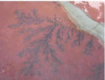
than those formed from biological growth processes, often exhibiting long fingers, deep fjords and fractal branching structures (see Figure 1).

Figure 1. A “pseudo fossil” formed by the deposition of manganese oxide in a sandy substrate. This illustrates the typical features present in clusters formed through mineral aggregation. (Photo: Alan Dickinson).

Discrete models

The earliest mathematical models for random growth were discrete in nature. In discrete models, growing clustersK₀ ⊂K₁ ⊂ · · ·are constructed as increasing sets of connected vertices on an underlying (infinite) connected graphG =(V,E). At each time step a new vertex is chosen from the neighbours of the cluster according to some stochastic rule and added to the cluster. To be precise, for any∅ ⊂A⊂V, let

∂A={v ∈V \A:(u,v) ∈E for someu ∈A}

denote the boundary of the subgraphAand suppose pA:∂A→ [0,1]is some function which satisfies

Õ

v∈∂A

pA(v)=1.

A random growth processK0,K1, . . ., of sets of

con-nected vertices, can be constructed recursively by starting from some connected set∅ ⊂K0⊂V and

takingKn+1=Kn∪ {v}with probabilitypKn(v). It is usual to start withK0={v0}wherev0 is some

dis-tinguished vertex called the seed particle. Typically G is a lattice such asZd andv0 =0.

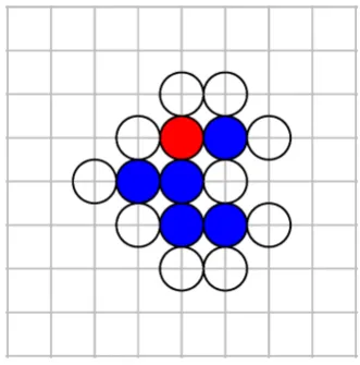
Figure 2. A representation of a random cluster grown on Z2. The red disk represents the seed particle which was placed at the origin. The blue disks are the first five particles to be attached to the cluster. The empty black circles represent the possible locations at which the next particle might be attached.

In order to model the physical growth processes dis-cussed in the previous section, we need to show how to construct probability distribution functionspA

which correspond to the physical attachment rules described above. We begin by considering biological

growth. One possible way to model uniformly ran-dom reproductive events on the cluster boundary is by choosing each successive particle uniformly from all possible locations on the boundary i.e. pA(v) =

1/|∂A| for eachv ∈ ∂A. This model is called the Eden model and was first proposed in 1961 [1]. This is not the only way in which biological growth can be modelled on a lattice. Observe that in Figure 2, the vertex at position(1,−1)has three possible parents whereas the vertex at position(2,0) has only one possible parent. If the new particles are actually aris-ing as offspraris-ing of the parent particles, one would expect the next particle to be more likely to be added at(1,−1)than(2,0). A more realistic variation on the Eden model is to pick each vertex with a probability which is proportional to the number of edges which connects that vertex to the cluster i.e. if

NA(v)={u ∈A:(u,v) ∈E},

then

pA(v)=

|NA(v)|

Í

u∈∂A|NA(u)|

.

In 1981, Witten and Sander proposed the following model for mineral aggregation which they called diffusion-limited aggregation or DLA [6]. As before, initialise with a seed at the origin or some other dis-tinguished vertex. At each time step place a particle on a random site at a large distance from the seed. Allow the particle to perform a simple random walk on the graph until it visits a site adjacent to the clus-ter at which point attach the particle to the clusclus-ter i.e. add the vertex on which the particle stopped. The distribution functionpA can therefore be obtained

by computing the hitting probabilities of the clus-ter boundary∂Aby a simple random walk started at “infinity”. In order to guarantee that the particle eventually reaches the cluster we need the random walk to be a recurrent process on the underlying graph. This means that ifG = Zd, we must take d ≤ 2. The case d = 1 is not very interesting as particles will always just attach to the left or right of the cluster with equal probability, so it is usual to taked =2when talking about DLA. A variant of this model is called multi-particle DLA in which infinitely many particles are simultaneously released from ran-dom positions, rather than one at a time, and they perform independent random walks until they hit the cluster. Computing pA explicitly for larger and

In order to model clusters formed by electric dis-charge, the notion of electric potential is needed. For simplicity, takeG =Z2 andv0 =0. Suppose there

are two electrodes in the system: one placed at0 and the second modelled as a large circle of radius R. LetBR(0) ⊂R2denote the open ball with centre

0and radiusR. Given a conducting cluster{0} ⊆ A⊂BR(0) ∩Z2, the electric potential is a discrete

harmonic functionφA (see the aside on “Harmonic

functions”) defined on the lattice withφA(v)=0if

v ∈ A and φA(v) = 1if |v| ≥ R. (It follows from

the discussion on harmonic functions thatφA(v)is

equal to the probability that a simple random walk started atv exits the ballBR(0)before hitting the

setA.) The probability of attaching a particle at a vertexv ∈∂Adepends on the local electric field, or potential difference,φA(v) −φA(u)=φA(v)for each

u ∈NA(v). Fixη ∈R. For eachv ∈∂A, let

pA(v)=

|NA(v)|φA(v)η

Í

u∈∂A|NA(u)|φA(u)η

.

This model is called dielectric-breakdown or DBM(η) and it was proposed in 1984 by Niemeyer, Pietronero and Wiesmann [3]. The parameterη determines the extent to which the attachment locations are influ-enced by the electric potential. In the case when η =0, this model is just the variation of the Eden model described above; whenη=1it produces clus-ters which are believed to behave qualitatively like DLA; asη→ ∞growth concentrates at the point of maximal potential difference. It is conjectured that the limit in this case is a simple path. Similarly to DLA, computingφA (and hencepA) explicitly becomes

in-creasingly complicated as the cluster grows.

Conformal models for planar random growth

The discrete models defined above are challenging to study, in part due to a lack of available mathematical tools. In 1998 Hastings and Levitov [2] formulated an approach to modelling planar growth, which included versions of the physical models described above. The idea was to represent growing clusters as composi-tions of conformal mappings. This approach provided a way in which techniques from complex analysis could be used to study planar random growth. LetK0 denote the unit disk in the complex planeC

and letD₀ =C\K₀. A particle is any compact set P ⊂D0 such thatK0∪P is simply connected. By

the Riemann mapping theorem (see the aside) there exists a unique conformal bijectionfP :D0→D0\P

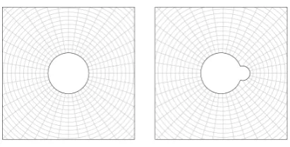
which fixes infinity. We use this mapping as a mathe-matical description of a particle attached to the unit disk. We say that the particle is attached at1if1lies in the closure ofP. Examples of allowable particle shapes include a bump, as shown in Figure 3, a disk tangent to the unit circle at1, or a slit (line segment) of the form(1,1+d]. IfP represents a particle at-tached at1, theneiθ_{P represents a particle of the}

same shape attached ateiθ_{. It has corresponding}

conformal mapping

feiθ_P(z)=eiθfP(e−iθz).

Figure 3. The exterior unit disk and its image under the conformal mapping corresponding to a single particle attached at1.

The Riemann mapping theorem

LetK ⊂Cbe a connected compact subset of

C, larger than a single point, such thatC\K is simply connected. There exists a unique con-formal bijectionf :D0→C\K which fixes

infinity in the sense that, for someC >0, f(z)=C z +O(1)as|z| → ∞.

Given a sequence of particlesP1,P2, . . . and their

associated conformal mappings f1,f2, . . ., define a

sequence of conformal bijectionsΦn:D0→C\Kn

by settingΦ₀(z)=z and recursively defining

Φ_n(z)=Φ_n−1◦fn(z)=f1◦ · · · ◦fn(z).

Note thatKn =Kn−1∪Φn−1(Pn), so the sequence

K0 ⊂K1 ⊂K2 ⊂ · · · represents a growing cluster

where the unit diskK0 is the seed particle and at

timenthe particleΦ_n−1(Pn)is added to the cluster

(see Figure 4).

particle. For each particlePn, letθndenote the

at-tachment angle anddn the diameter. By choosing

the sequencesθ1, θ2, . . . andd1,d2, . . . in different

ways, it is possible to describe a wide class of growth models. In the remainder of this section, we will ex-plore how to choose these sequences in order to construct models that correspond to the physical processes described in the first section.

Figure 4. An example of a clusterKn, grown by successive compositions of conformal mappings, together with the image of the exterior unit disk under the mapΦ_n. The seed particle is shown in red and the first five particles to arrive are shown in blue.

In the model for biological growth, the probability of attaching a particle along a section of the cluster boundary should be proportional to the arc-length along that section of the boundary. Specifically, given an open arc in∂Kn−1, there exista <b ∈ Rsuch

thatθ7→Φ_n−1(eiθ)maps the interval(a,b)onto this

arc. The length of this arc is therefore given by

∫ b

a

|Φ0_n−1(eiθ)|dθ.

Attaching the next particle onto this arc is equivalent to pickingθn ∈ (a,b)and so we need

P(θn ∈ (a,b)) ∝

∫ b

a

|Φ0_n−1(eiθ)|dθ

or equivalentlyθnmust have density function

propor-tional to|Φ0

n−1(e

iθ_{)|. Next consider how the diameter}

dn should be chosen. For simplicity suppose that

the particle being attached is a small slit of length

dn i.e.Pn =eiθn(1,1+dn]. In this case, an explicit

formula can be written down for the function fn(see

[2]). Furthermore, there exists someβn(which can be

expressed as a function ofdn) such thatθ7→fn(eiθ)

maps the interval(θn, θn+βn]toPn. Using the chain

rule, the particle Φ_n−1(Pn) which is added to the

cluster therefore has length

∫ βn

0

|Φ_n0₋₁(fn(ei(θn+θ)))||fn0(ei

(θn+θ)

)|dθ.

Since

dn=

∫ βn

0

|fn0(ei(θn+θ))|dθ,

the length of Φ_n−1(Pn) is approximately equal to

dn|Φ0_n−1(rneiθn)| for some1 ≤rn ≤ 1+dn. In the

physical models, the particles being attached are all the same size, sayd. We therefore need to choose dnin such a way as to ensure that this expression is

approximately equal tod for alln. Whend is small, a possible choice is to take

dn=d|Φn0−1(eiθn)|

−1_{. (1)}

The above choices ofθn anddnprovide a model for

an off-lattice version of the Eden model.

Now suppose we wish to construct an off-lattice ver-sion of DLA. Exactly the same argument as above shows that we should again choose dn satisfying

(1). However, this time we need to pickθn so that

Φn−1(eiθn)has the same distribution asWτ where

Wtis a Brownian motion started from infinity (viewed

on the Riemann sphere) andτ is the first time that the Brownian motion hits Kn−1. Equivalently, eiθn

should be the hitting distribution ofΦ−_n−1₁(Wt)on the

unit circle. However, Φ−1

n−1 is a conformal mapping

and therefore its real and imaginary parts are har-monic functions (see the aside). Using Itô’s formula,

Φ−1

n−1(Wt)is a continuous martingale and hence is

a time-change of Brownian motion. By symmetry, the hitting distribution of a time-change of Brownian motion on the unit circle is uniform, soθnshould be

chosen with the uniform distribution on[0,2π). A similar argument can be used to show that one can obtain an off-lattice version of DBM(η)by taking θnwith density function proportional to

|Φ_n0₋₁(eiθ)|1−η

anddnsatisfying (1). Note that, as in the discrete case,

η = 0corresponds to the Eden model and η = 1 corresponds to DLA. There are several variations on this. In the original Hastings-Levitov model HL(α) [2], θnis picked uniformly on the unit circle and

dn=d|Φ_n0−1(e

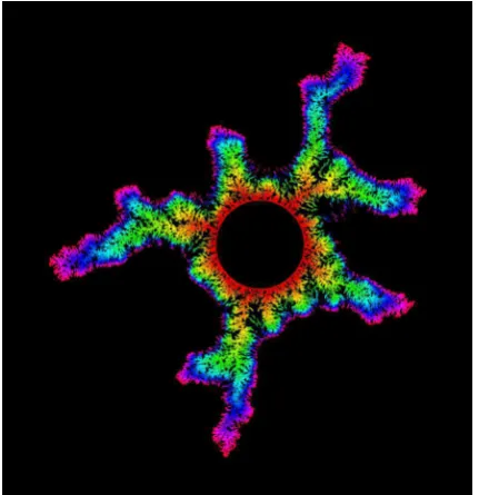
The HL(α) model corresponds to DBM(η) via the re-lationα=η+1so HL(2)gives DLA (see Figure 5).

Figure 5. A version of DLA grown by composing conformal mappings using the Hastings-Levitov construction.

Mathematical study of random growth

Random growth clusters in the physical world usually consist of a large number of particles, each of which is small relative to the size of the cluster. Although the randomness typically occurs at a microscopic level through the attachment rule for each successive par-ticle, we observe the clusters at a macroscopic level where we cannot see the individual particles. Ran-dom growth processes are completely unpredictable at the level of particles, however large clusters of-ten exhibit predictable or ‘universal’ behaviour. The aim of studying mathematical models is to extract the principle mechanisms underlying this universal behaviour.

One of the intriguing features of random growth mod-els is that, even though the modmod-els are isotropic by construction, simulations suggest that large clusters become anisotropic (see Figure 5). As yet there is no satisfactory mathematical explanation for how such complicated structures arise from the dynamics of the model. Representing random growth clusters using conformal mappings enables one to combine analytic and probabilistic techniques. Research at the interface of these two fields has already given us mathematical objects such as stochastic partial

dif-ferential equations (SPDEs) and stochastic Loewner evolution (SLE). The recent developments in these ar-eas have suggested approaches and techniques that can be applied in a random growth setting and we are beginning to be able to identify the characteristics of random growth in specific cases [5, 4].

It has been over fifty years since mathematicians and physicists first started seriously thinking about random growth. Although progress has been made in this time, we are still some way from being able to answer the really important questions. Mathematical tools and techniques that may shed light on these questions have recently started to emerge. There is a good chance that we will not need to wait another fifty years for the major breakthrough, so right now this is a very exciting area to be involved in.

REFERENCES

[1] M. Eden, A two-dimensional growth process, Proc. 4th Berkeley Sympos. Math. Statist. and Prob. (1961) 223–239.

[2] M. B. Hastings and L. S. Levitov, Laplacian growth as one-dimensional turbulence, Phys. D 116 (1998) 244–252.

[3] L. Niemeyer, L. Pietronero, and H. J. Wiesmann, Fractal dimension of dielectric breakdown, Phys. Rev. Lett. 52 (1984) 1033–1036.

[4] J. Norris, V. Silvestri, and A. Turner, Scaling limits for planar aggregation with subcritical fluc-tuations, Preprint 2019, arXiv:1902.01376.

[5] A. Sola, A. Turner, and F. Viklund, One-dimensional scaling limits in a planar Lapla-cian random growth model, Preprint 2018, arXiv:1804.08462.

[6] T. A. Witten Jr., L. M. Sander, Diffusion-limited aggregation: a kinetic critical phenomenon, Phys. Rev. Lett. 47 (1981) 1400–1403.

Amanda Turner

Harmonic functions

A continuous functionu : ¯D → R, whereD is some open subset of Rd andD¯ is its closure, is a harmonic function if it satisfies Laplace’s equation

∆u =0inD (2)

where

∆u =∂

2_u

∂x2 1

+· · ·+∂

2_u

∂x2

d

.

Using the Cauchy-Riemann equations, it can be shown that the real and imaginary parts of any holomorphic function are harmonic functions. Harmonic functions are closely connected with Brownian motion. LetDbe a transient domain (i.e. a domain which Brownian motion will exit in finite time almost surely). Then ifu is a harmonic function onD

u(x)=Exu(Wτ) (3)

whereW is ad-dimensional Brownian motion started atxandτ=τD is the first exit time fromD. Set

ω(x;dy)=Px(Wτ∈dy).

Then we can write (3) as

u(x)=

∫

∂D

u(y)ω(x;dy).

We callω(x;dy)the harmonic measure on∂Das seen fromx. Using the symmetry of Brownian motion, it follows that harmonic functions satisfy the mean value property

u(x)=

∫

∂Br(x)

u(y)dA(y)

for all ballsBr(x) ⊆D, wheredAis the normalised uniform surface area measure on∂Br(x).

A similar notion, with analogous properties, exists on a graphG =(V,E). Given any finite connected subgraph∅ ⊂D ⊂V, a functionu :D∪∂D→Ris discrete harmonic onDif it satisfies (2), where∆

is now the discrete Laplacian

∆u(x)= Õ

y:(x,y)∈E

(u(y) −u(x)).

This implies the mean-value property

u(x)= 1 |∂{x}|

Õ

y:(x,y)∈E

u(y).

For anyA ⊂ ∂D, the harmonic measure ofA with respect toD, ω(x,A,D), is the unique discrete harmonic function onD with boundary valuesω(x,A,D)=1whenx ∈ Aandω(x,A,D)=0when x∈∂D\A. Harmonic measure is closely connected with simple random walks via the relationship

ω(x,{y},D)=Px(Xτ =y)

whereXn is a simple random walk starting fromx andτ=τD is the first exit time fromD. Ifu is any

harmonic function onD then

u(x)= Õ

y∈∂D