On the Quantization of One-Dimensional Conservative
Systems with Variable Mass
G. V. López
Departamento de Física de la Universidad de Guadalajara, esq. Calzada Olmpica, Guadalajara, México
Email: [email protected]
Received May 30,2012; revised June 25, 2012; accepted July 18, 2012
ABSTRACT
The Hamiltonian associated to the mass variable system is constructed from first principles through finding a constant of motion of the system. A comparison is made of the classical motion of a body with its mass position depending in the (x,v) space and (x,p) space which are defined by the constant of motion and the Hamiltonian, for a particular model of mass variation. As one could expected, these motion looks different on these spaces. The quantization of the harmonic oscillator with this mass variation is done, and a comparison is made by using the usual Hamiltonian approach with the proposed quantization of the constant of motion approach. This comparison is done at first order in perturbation theory, and one sees a difference between both approaches which can, in principle, be measured.
Keywords: Mass Variation; Quantization; Constant of Motion; Hamiltonian
1. Introduction
Mass variation problems for classical mechanics has a long history [1] and important applications have been studied on the dynamics of the Universe as black hole formation [2,3], where they have been known as Gylden- Meshcherskii problems [4-11]. These types of problems are not free from controversy in the way they must be formulated and their relation with Galileo’s transforma-tion [12]. In additransforma-tion, these systems are becoming more and more important in quantum mechanics systems since the discovery of the neutrinos mass oscillations problem [13] and [14], the kinetic theory of dusty plasma [15], propagation of electromagnetic waves in a dispersive- nonlinear media [16], and other possible applications in fluid dynamics [17].
The approach used so far to study these systems fol-lows guessed Lagrangian or Hamiltonian with include the mass variation of the system [18-20]. Above all, there is not right mathematical justification for this approach. Therefore, one may considered that to find the Hamilto-nian for a mass variation system, one must do it from first principles, Newtonian’s mechanics, and this can be done by using a well known approach for one dimen-sional autonomous system to construct the associated Lagrangian and Hamiltonian of the system [21-23]. Once these expressions are gotten, one can proceed to make the quantization of the system [24]. On the other hand, there has been a proposed extension for the non
relativis-tic quantum mechanics for autonomous systems based on the use of the constant of motion instead of the Hamilto-nian in the Schrödinger equation [25]. Therefore, in this paper the Hamiltonian and the constant of motion are found for several conservative systems with position de-pending mass, using a model for the mass variation. The trajectories of the motion on the (x,v) and (x,p) spaces are shown to see the difference of this description. The quan-tization of the mass position depending systems is ana-lyzed using the constant of motion and the Hamiltonian approaches, and finally, the spectrum of the harmonic oscillator are calculate at first order perturbation theory.
2. Constant of Motion and Hamiltonian
Consider a one-dimensional motion of a body with mass position depending, m=m x
, and which is affected bya conservative force F x
. This system is governed byNewton’s equation of motion [1]
d
= ,
d mv
F x
t (1)
where v represents the velocity of the body. Since one has the expression
d = ,
d x
m m v
t (2) where one has defined mx= dm xd , the equation of
=
2,x
F x m v d
d v m x
t (3) which in turns, this equation can be written as the fol-lowing autonomous dynamical system
2F x = , =
x v v x v
m (4)
where has defined as
x =m mx .> 0 v < 0
v
, (5) This autonomous system is dissipative for and anti dissipative for because of the quadratic term in the velocity. A constant of motion of this system is a function K x v which satisfies the first order partial
differential equation
2 = 0.K K
x v v
=F x v
x m x (6)
The general solution of this equation is given by
K G C
, where G is an arbitrary function, and C is the characteristic curve given by
2 d0 d 0 .
x s
s e
2 d 2
= 2
s s F s
C v e
m s
m x
(7)Suppose of the form
=m g x
g
o ,
where one demands that . In addition, assum-ing that , one gets the usual constant of motion of the conservative system with constant mass (so called “Energy of the System”). Then, one can select the func-tionality of G of the form
m x
0 = 0 g 0
= ,
2
o
m
G C C (8)
such that under the mentioned conditions for g, one gets the energy of the system as a particular limit. The result-ing constant of motion of the system is
0
d 2 0 d .x s
s e
2 d 2
1
, =
2
s s
o o
F s
K x v m v e m
m s
(9)Given the constant of motion of a one-dimensional autonomous system, the Lagrangian for this system is determine through the well known expression ([21-23])
2, d . K x , =
L x v v
(10) Using this expression with Equation (9), it follows that
0
d 2 0 d .x s
s e
2 d 2
1 , =
2
s s
o o
F s
L x v m v e m
m s
(11)The generalized linear momentum, =p L v
2 d 0
= ,
x s s
o p m ve
=
, is given by
(12)
H vp L
and the Hamiltonian of the system, , is de-duced as
,
= 2 2 0 d d 2 0 d .2
x s
s s
o o
F s s
p
H x p e m e
m m s
(13) Since from Equation (5) one has that
0 d = ln ,
x
o
m x
s s
m
(14)
The constant of motion, Lagrangian, generalized linear momentum, and Hamiltonian are written as
2 2
0
1
, = d ,
2
x
o o
m x
K x v v m s F s s
m m
(15)
2 2
0
1
, = d ,
2
x
o o
m x
L x v v m s F s s
m m
(16)
2
, = ,
o
m x
p x v v
m
(17)
and
2
2 0
1
, = d .
2
x o
o
m p
x p m s F s s
m
m x
H (18)
Defining the effective potential as
01
= x d ,
eff
o
V x m s F s s
m
(19) the constant of motion and Hamiltonian have the follow-ing form
2 2
, =
2 eff
o
m x
K x v v V x
m
(20) and
2 2
, = .
2
o
eff
m
H x p p V x
m x
m x(21) To be able to continue with analysis, one needs a model for the variation of mass, . Let us assume that m x
is given by
1
1
= 1 x x ,
o
m x m m e (22)
0 =mom and
where m
=m1, and x1 d termines theasymptotic distance where the mass would be mo m1
e
. ll have and increasing of mass going from x= 0
to x> 0 m1> nd vi a if m1< 0. For this
The effective potential is given by One wi
if 0, a se vers model,
1
1
0
= x s x d ,
eff
o
m
V x V x V x e F s s
m
where V x
is the usual conservative potentiale force
due to
F x ,
The trajectories in the space
,
= 0x
d .V x
F s s (24)th
x v are d
the constant of m Equation (20), traje
etermined by given the initial otion
conditions x
0 and v
0 . The ctories in the space
x p,
are determined by Equation (21) with the initialconditions x
0 and p 0
, where Equation (17)re-l oth initial conditions. Figures 1 and 2 show the trajectories in e space
,
s b ate
th x v and
x p,
for acon-stant force F x
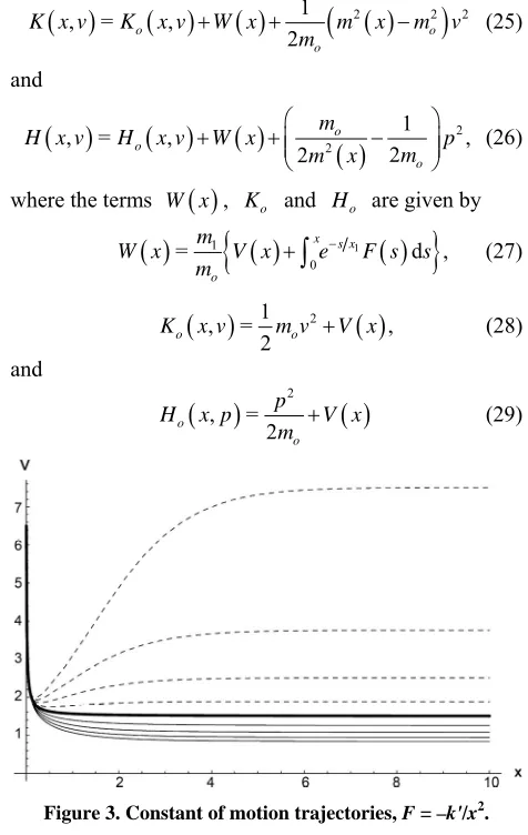
= f . Figures 3 and 4 show the trajec-tories in the spaces
x v, an d
x p,
fo a CoulombForce
r
2 =
F x k x (zero potential is taken at =x ). Figures 5 and 6 show the trajectories in the spaces
x v,and
x p,
for the Hook’s law (harmonic os )
=cillator
F x kx (for the dissipative case v> 0).
continu black line represents m1= 0, dotted lines
corres o m1< 0 and continuous lines t m1> 0.
The following values have been us ake this plots (units MKS), m g, x1= 10 m, x
0 = 0 m,
Gross o
ous
pond t
ed to m
= 10 K
o
0 = 1.5 m s ,
v f = 10 Newtons, and k= = 1k (in their
respective units).
Figure 1. Constant of motion trajectories, F = f.
Figure 2. Hamiltonian trajectories, F = f.
As one can see from these plots, the effect of the first terms in Equations (20) and (21) is clearly marked on these trajectories. The constant of motion brings about some “regular” behavior meanwhile the Hamiltonian brings about some type of little odd behavior due to ex-pression (17).
From Equations (23), (20) and (21) one sees that the constant of motion and the Hamiltonian can be written as
, =
,
1
2
2
22
o o
o
K x v K x v W x m x m v
m
(25)
and
22
, = , ,
2 2
o o
o
1 m
H x v H x v W x p
m
m x
(26)
where the terms
W x , Ko and Ho are given by
1
1
0
= m x s x d ,
W x V x e F s s
m
(27)o
, =1 2
,2
o o
K x v m v V x (28)
and
,
= 2
2
o
o
p
H x p V x
[image:3.595.303.541.189.565.2]m (29)
Figure 3. Constant of motion trajectories, F = –k'/x2.
Figure 5. Constant of motion trajectories, F = –kx.
Figure 6. Hamiltonian trajectories, F = –kx.
This form of writing the constant of motion and the Hamiltonian is suitable for quantization studies. Before leaving this classical part, it is necessary to make some observations about the motion of the body and its mass position dependence. First, in our mass position depend-ence model, Equation (22), it has been assumed that the
ptotic (x1) mass valu n by mo m1
asym e is give . If
dy oscillates (harmonic r), in addition to ing-antidamping effect d e term with 2
v in
ion (3), one must consid ffect of decreasing
> 0
v ) and in (f ) of mass effect
these oscillatio . Seco e would like to
e
scilla-the bo damp Equat (for during
nsid ons, i
oscillato ue to th
er the e or v< 0
nd, if on creasing
ns co
ti
r pure decreasing of mass during these o t is necessary to change the model for m x
.Third, if one wants to consider pure damping effect dur-ing these oscillations, this will only happen if m x
< 0for v< 0 and m x
> 0 for v> 0, [26]. Finally, if
> 0m x (our model) or m x
< 0 for any position“x”, the damping-antidamping effect will appear.
3. Quantiz
n with Mass Position
Depending Systems
The usual Schrödinger quantization approach is based on the association of an Hermitian op r to the Hamilton
function, [27,28], and the solution of a linear complex partial differential equation for the wave function,
atio
erato
x t, ,
ˆ
= , ,
i H x p ) is the Hermitian o associated to the generalized linear momentum,
t
(30
where pˆ perator
ˆ =
p i x, is the
Plank constant divided by 2π, having the confutation relation
x p,ˆ =i I (with “I” the identity obasis
perator) in the
I x p, ,ˆ
of the Weyl algebra. However, as aion fun
for the wave function,
possible extension of this quantization approach, there is the proposal of using the constant of motion, instead of the Hamiltonian, in the Schrödinger equation, where an Hermitian operator is associated to the constant of mo-t ction, and the Schrödinger like equation is solved
ˆ= , ,
i K x v (31) or associ d
t
where ˆv is the Hermitian operat ate to the velocity, vˆ =i
m
x, satisfying the obvious com-mutation
relationˆ
, = .
x v i I
m
(32) These realtions can be assumed to be valid for position mass depending as
ˆ= , and ,ˆ = .
v i x v i I
m x x
(33)
m x
Of course, for constant mass conse
there is not difference at all between both approaches he
nd the velocity
r, as we have seen previously, for mass position depending systems this relation is not trivial any more, Equation (17). Therefore, to fin
for the quantization of the constant of motion to make ph
rs, and to see experimentally whether or not it makes sense. Mass position depending systems have indeed this property because of th
tion (17).
ven
rvative systems, since t relation between the generalized linear mo-mentum a of the body is really trivial,
= o
p m v. Howeve
d out the possibility ysical sense, it is necessary to look for a system where both approaches diffe
[image:4.595.57.290.61.432.2]
1 12 2 2 1 2 1 1 1 , , 2 o om m x
K x v K x v W x x m v
x m x
(34) and
2 2 2 1 1 12 2 1 1 , , 2 3 1 2 2 o
o o o o
H x p H x p W x
m m m x
x p
m m x m m x
(35) where the function W x
is defined as m1 1 x
d 1 x 2
d .W
sF s s 2
s F s s (36)0 0
1 1
o
m x x
To associate a Hermitian operator to these functions, one knows that there is an ambiguity, not resolved yet by any experiment, on selecting a proper Hermitian ope to make the quantization. Although one could norm follow Weyl approach [29] and [30], it is easier to take
wing approach by noticing the following for polynomials operators: given the Herm operators ˆ
rator ally the follo
itian A
and Bˆ to the functions A and B, the operator
AˆBˆ
nis an Hermitian operator for any mber “n
ing H
asso-ciated to the product of functions
integer nu ”. In this way, the follow ermitian operators can be
=1 ˆ
ˆ ˆˆ
, 2AB ABBA (37) 2=1
ˆ2ˆ ˆ ˆˆ ˆˆ2
,3
AB B ABABAB (38) and
2 2
2 2 2 2 2 2
1 ˆ ˆ ˆ ˆ ˆ ˆˆ ˆ ˆ ˆˆ ˆ ˆˆ ˆ ˆˆ ˆ
= .
6 A B
A B B A ABABBABABA BAB A
) Taking the following identifications ˆ =
(39
A x and ˆ= ˆ
B p or vˆ, it follows that the Hermitian operators
associated to the expressions (34) and (36) are given by
1 1 2 1 1 2 12 2 2 2 2 2
ˆ ,ˆ = ˆ ,ˆ ˆ
3
12
ˆ ˆ ˆ ˆ ˆ ˆ ˆ ˆ ˆ
o
o
m 2 2 ˆ2 ˆ ˆ
K x v K x v W x x v
x
m m m
x
v x vxv
x v v x xvxv vxvx vx v xv x
and (40)
1 2 1 1 2 2 12 2 2 2 2 2
3 1
12 2
ˆ ˆ ˆ ˆ ˆ ˆ ˆ ˆ ˆ
o o o o m m m
m x m
2 2
1 2
ˆ ,ˆ = ˆ ,ˆ ˆ ˆ ˆ ˆ
3
.
o
m
H x p H x p W x p x pxp xp
m x
x p p x xpxp pxpx px p xp x
(41)
Using the commutation relations
x p,ˆ =i I and
1 12 1 22 2
1 1
ˆ
, = ,
with = 1 ,
2
o
o o o
x v i f x
m
m m m x
f x x
m x m m x
gets the following expressions for the constant of motion and Hamiltonian operators
(42) one
2 2 1 1 2 1 1 2 2 2 2 2 2ˆ ,ˆ = ˆ ,ˆ
ˆ ˆ ˆ
, 3 3 ˆ ˆ 2 6 6 ˆ ˆ , 6 6 o o o o o o
o o o
K x v K x v W x
m i i
x v D x fv f x v
x m m
m m m
i
1
2x
x v xf x g x v h x
m m
i i
xf x v xD x f v xg
m m m
x
(43) and
2
1 2 1 2 2 2 2 1 1 2 2 1
ˆ ,ˆ = ˆ ,ˆ ˆ 2 ˆ
3
1 ˆ ˆ
2 , 2 2 2 o o o o o m
H x p H x p W x xp x i xp
m x
m m
x p i xp
m
m x m
(44) where the functions f
x and h x
, and the operator
, ˆ
D x f v have been defined as
1
12 1
2 2
1 1
2 =
2
o o o
xf x
m m m
g x f x
m x m m x
(45)
2 1 1 1 2 2 2 1 = 1 2 2 o o o m mh x m m x g x
m m
xg x f x
x (46)
1
12 1
2 2 1 1 ˆ , ˆ = 2
o o o o
D x f v
xf x
m m m
i
f x v f x
m m x m m x
(47)
ns (3 (31)
mous sys se equation are reduced
to the solution of eigenvalue problems
Now, since Equatio 0) and represent autono-tems, the solution of the
ˆ ,ˆ =
H H H
H x p E and
(48)
ˆ ,ˆ = .
K K K
Considering on Equations (43) and (44) that the terms appearing on the right hand side are small with respect the terms Kˆo and Hˆo, the modification of the Kˆo and Hˆo sp
bation di st have that
for bot
ectra can be calcu order in pertur theory to see whether or here is a sig-nificant fference in their predictions his case, one
u the eigenfunctions and alues are the same h app when m1= 0
0 = 0 0.
n n
E
(50)
lated just at first not t . In t eigenv
, m
roaches
0 0 0
ˆ = , and ˆ
o n n n o n
H E K
Then, at first order perturbation theory, the eigenval-ues would be given by
1 = 0 ˆ
EH En n W n n H n (51) and
I
1 0
K n
E =E n W n n K nˆI , (52)
where n W n =W is the expe function W in the state nn n0 , and ˆ
ctation value of the I
K and HˆI
rep-resent the remaining terms of the Equations (43) and (44),
1 2 2 2 2 ˆ ˆ 2ˆ , ˆ
6
o o
i
x v xf x g x v h
i 2 2 1 1 2 1 1
ˆ = ˆ , ˆ ˆ
3 3 2 I o o o
m i i
K x v D x f v f x v
x m m
m m m
x 2 6 6 o o m m i 2 6 o x xf x
v xD x f v xg x
m m m (53) and
2
1 2 1 2 2 2 1 1 2 2 3
1 ˆ ˆ
2 .
2
2 2
I
m m
x p i xp
m
m x m
2
1
ˆ = ˆ 2 ˆ
o
o
o o
m
H xp x i xp
m x
4. Harmonic Oscillator with Variable Mass
The harm m1= 0 in the Weylalge-sis , ,
(54)
onic oscillator with
†
bra ba I a a [31] has the following
characteris-tics
0
2 ,
0 = ,n
†
ˆ = ˆ = , = 1
o o n
K H a a E n n (55)
with the following identifications
† † , 2 2 = , 2 o o o m † ˆ = , = ˆa a p i a a
M
v i a a
m
and having the well known properties
†
†
= , = 1 1 , =
and , = .
nm
n m a n n n a n n n
a a I
(57) s and x (56) 1 ,
Note that all the expectation values of monomial term of odd power have zero values. The expression for W
n by
up to fourth order in “x” is give
3 4 1 1 km km 2 1 1 = .
2 o 8 o
W x x
m x m x (58)
Thus, using the expectation values given in the ap e terms appearing in Equations (53) and (54) can be calculated, resulting the following eigenvalues at first order
pen-dix, the expectation value of th
2
1 0 1 2
2 1 2 1 1 2 2 1 1
= 6 6 2
2 8 ˆ 2 K n o o o n o o o km
E E n n
m m x m m v m x m (59) and 1 2 ˆ , 3 n m m
i D x f v f
m x
2 1 2 1 1 2 2 2 ˆ ˆ 6 n n o o n n o o km f vm m m
1 0 1 2
2 1
1 2
= 6 6 2
2 8 ˆ , 3 K n o o
E E n n
m m x
m
i D x f v
m x
1
2 2
2 2
ˆ ˆ ˆ
2 6 o o n n n o m x m i
x v xf v gv
m i
h x xf v
m m (60) 2 2
6 n 6 n
o o i xD xg m m
where one has used the definition n= n n . Let us define the following parameter J as
2
1 0 1 2
2 1 2 2 2 1 1 2 2 1
= 6 6 2
2 8
3
2 1 ,
8 2 H n o o o o o km
E E n n
m m x
m m
n m
m x m
(61)
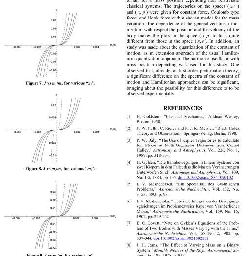
This parameter represents the relative variation of the eigenvalues of the constant of motion quantization and the Hamiltonian quantization approaches. Figure 7 shows this parameter as a function of m m1 o (relative change
of mass), considering that =10 Kg,24
o
9
= 10
8
1= 10
Hz, and = 0n (ground state), for x m j = 1 (dotted lin rogressively).
shows J as with j
Figure 8
e), 2, 4, 6, and 8 (p tion of
a func m m1 o considering
th previous valu e parameters but for j = 1
= 1
m j j= 1 (dotted line), 20, 40,
. Fi J vs
e same and o
and 80
es for th
Kg with shows ag
24
0
gure 9
60 ain m m1 o with the
values ters as before but with
and line), 2, 4, 6, a
se n for a rela
body, the difference of same
= =
j j As one ca sma
for the parame = 0 (dotted these
ass of 1
n
for n e from n the m
nd 8. tively plots, eve
the ll change i
rious “x1”. Figure 7. J vs m1/mo for va
[image:7.595.48.547.205.731.2]Figure 8. J vs m1/mo for various “mo”.
Figure 9. J vs m1/mo for various “n”.
the eigenv be
rela-vely large. Thus, this suggest the it can be observable perimentally, opening up the possibility to see whether or not the quantization of constant of motion makes sense for mass variable quantum systems.
5. Conclusion
A mathematical consistent approach has been used to deduce the constant of motion, Lagrangian, and Hamil-tonian for a mass position depending non relativistic classical systems. The trajectories on the spaces ( ,
alues for both approaches (J) could ti
ex
x v)
and (x p, ) were given for constant force, Coulomb type
force, and Hook force with a chosen model for the mass variation. The dependence of the generalized linear mo
mentum w f the
ody makes the plots in the space ( ,
-ith respect the position and the velocity o
x
b p to look quite
ifferent from those in the space ( ,
d x v). In addition, an
study was made about the quantization of the constant of motion, as an extension approach of the usual Hamilto-nian quantization approach The harmonic oscillator with mass position depending was used for this study. One observed that, already, at first order perturbation theory, a significant difference on the spectra of the constant of motion and Hamiltonian approaches can be significant, bringing about the possibility for this difference to to be observed experimentally.
REFERENCES
[1] H. Go on-Wesley,
istances from Comet Halley,” Astronomy and Astrophysics, Vol. 226, No. 1,
34.
ldstein, “Classical Mechanics,” Addis Boston, 1950.
[2] F. W. Helhl, C. Kiefer and R. J. K. Metzler, “Black Holes: Theory and Observation,” Springer-Verlag, Berlin, 1998. [3] P. W. Daly, “The Use of Kepler Trajectories to Calculate
Ion Fluxes at Multi-Gigameter D 1989, pp. 318-3
[4] H. Gylden, “Die Bahnbewegungen in Einem Systeme von zwei Körpern in dem Falle, dass die Massen Veränderungen Unterworfen Sind,” Astronomy and Astrophysics, Vol. 109, No. 1-2, 1884, pp. 1-6. doi:10.1002/asna.18841090102 [5] I. V. Meshcherskii, “Ein Specialfall des Gyldn’s n
P lems,” Astronomische Nachrichten, Vol. 132, No. 3153, 1893, p. 93.
[6] I. V. Meshcherskii, “Ueber die Integration der Bewegung- sgleichungen im Problemezweier Krper von Vernderlicher Masse,” Astronomische Nachrichten Vol. 159, No. 15, 1902, pp. 229-242.
[7] E. O. Lovett, “Note on Gyldén’s Equations of the Prob- lem of Two Bodies with Masses Varying with the Time,” Astronomische Nachrichten, Vol. 158, No. 2, 1902, pp. 337-344.
che rob
,
doi:10.1002/asna.19021582202
[9] L. M. Berkovich, “Gylden-Meščerskii Problem,” Celes- tial Mechanics and Dynamical Astronomy, Vol. 24, No. 4, 1981, pp. 407-429. doi:10.1007/BF01230399
[10] A. A. Bekov, “Integrable Cases and Motion Trajectories
in the Gylden-M Soviet Astronomy
Vol. 33, 1989,
eshcherskii Problem,” pp. 71-78.
, [11] C. Prieto and J. A. Docobo, “Analythic Solution of the Two-Body Problem with Slowly Decreasing Mass,” As-tronomy and Astrophysics, Vol. 318, 1997, pp. 657-661. [12] G. V. López, “About Galilean Transformation on a Mass
Variable System and Two Bodies Gravitational System with Variable Mass and Dampen-Anti Damping Effect Due to Star Wind,” 2012.
http://arxiv.org/abs/1203.0495v1
[13] H. A. Bethe, “Possible Explanation of the Solar-Neutrino Puzzle,” Physical Review Letters, Vol. 56, No. 12, 1986, pp. 1305-1308. doi:10.1103/PhysRevLett.56.1305 [14] E. D. Commins and P. H. Bucksbaum, “Weak
Interac-tions of Leptons and Quarks,” Cambridge University Press, Cambridge, 1983.
[15] A. G. Zagorodny, P. P. J. M. Schram and S. A. Trigger, “Stationary Velocity and Charge Distributions of Grains in Dusty Plasmas,” Physical Review Letters, Vol. 84, No. 16, 2000, pp. 3594-3597.
doi:10.1103/PhysRevLett.84.3594
[16] O. T. Serimaa, J. Javanainen and S. Varró, “Gauge-Inde- pendent Wigner Functions: General Formulation,” Physi- cal Review A, Vol. 33, No. 5, 1986, pp. 2913-2927. doi:10.1103/PhysRevA.33.2913
[17] I. Ye. Terapov, “On Some Fundamental Problems of the Variable-Mass Continuum Mechanics,” International Jour- nal of Fluid Mechanics Research, Vol. 28, No. 4, 2001, pp. 152-174.
[18] C. Quesne, B. Bagchi, A. Banerjee and V. M. Tkachuk, Hamiltonians with Position-Dependent Mass, Deforma- tions and Supersymmetry,” Bulgarian Journal of Physics
amping Process: Application to , Vol. 33, 2006, pp. 308-318.
[19] Y. Hamdouni, “Motion of Position-Dependent Effective Mass as a Damping-Antid
the Fermi Gas and the Morse Potential,” Journal of Phys- ics A: Mathematical and Theoretical, Vol. 44, No. 38, 2011, Article ID: 385301.
doi:10.1088/1751-8113/44/38/385301
[20] M. Çapak, Y. Cançelik and Ö. L. Ünsal, S. Tay and B. Gönül, “An Extended Scenario for the Schrödinger Equa- tion,” Journal of Mathematical Physics,Vol. 52, No 2011, Article ID: 102102.
. 10, 1063/1.3646371 doi:10.
[21] J. A. Kobussen, “Some Comments on the Lagrangian Formalism for Systems with General Velocity Dependent Forces,” Acta Physica Austriaca, Vol. 51, 1979, pp. 293- 309.
[22] C. Leubner, “Inequivalent Lagrangians from Constants of the Motion,” Physical Review A, Vol. 86, No. 2, 1981, pp. 68-70. doi:10.1016/0375-9601(81)90166-3
[23] G. López, “One-Dimensional Autonomous Systems and Dissipative Systems,” Annals of Physics, Vol. 251, No. 2, 1996, pp. 372-383. doi:10.1006/aphy.1996.0118
[24] G. Lópezand and G. González,“Quantum Bouncer with Dissipation,” International Journal of Theoretical Phys- ics, Vol. 43, No. 10, 2004, pp. 1999-2008.
.c0 doi:10.1023/B:IJTP.0000049005.73750
[25] G. López and P. López, “Velocity Quantization Approach of the One-Dimensional Dissipative Harmonic Oscilla- tor,” International Journal of Theoretical Physics, Vol. 45, No. 4, 2006,pp. 753-742.
doi:10.1007/s10773-006-9064-9
[26] G. López, “Restricted Constant of Motionfor the One- Dimensional Harmonic Oscillator with Quadratic Dissi- pation and Some Consequences in Statistic and Quantum Mechanics,” International Journal of Theoretical Physics, Vol. 79, No. 4, 2001, pp. 71-79.
doi:10.1023/A:1011972700121
[27] A. Messiah, “Quantum Mechanics Vol. I,” John Wiley and Sons, New York, 1958.
[28] P. A. M. Dirac, “The Principles of Quantum Mechanics,”
. 1-46. 4th Edition, Oxford Science Publications, Oxford, 1992. [29] H. Weyl,“Quantenmechanik und Gruppentheorie,” Zeits-
chrift für Physick, Vol. 46, No. 1-2, 1927, pp doi:10.1007/BF02055756
[30] R. Kubo,“Wigner Representation of Quantum Operators and Its Applications to Electrons in a Magnetic Field,” Journal of the Physical Society of Japan, Vol. 19, 1964, pp. 2127-2139. doi:10.1143/JPSJ.19.2127
d F. Laloë, “Quantum [31] C. Cohen-Tannoudji, B. Diu an
Appendix
List of expectation values.
2k 1 ˆ2k 1
n = n = 0,
x v kZ (A1)
2lˆ2k 1 2k 1 2ˆl
n = n = 0, ,
x v x v k lZ
(A2)
= 2 1
2 o
x n
m
(A3) 2 n
24 = 6 2 6 2
x n n (A4) 2 n o m ˆ = 2 n o xv
m (A5) i
2
= 5n3
(A6) 3ˆ 2 n o
x v i
m
2
ˆ = 2 2 1
x v n n
2 2 2 2 4 n o
m
(A7)
1 1
2 2
1
= 1 2 1
o o
m m
f x n
m m
(B1)
2 1 2 2 n o m x
=
2 1
2
n
o o
m
xf x n
m x m
1
(B2)
1
2
2 1 1
2
2
2 1
=
2 2
6 6 2
n
o o o
n m m
x f x
m m m
n n (B3) 2 2 1 1
2mo
x
2 2 1 1 2 2 1 2 1 2 26 6 2
o o o m m m m m x n n 2 2
2 1 1 1
2 2 1 1 2 1 1 = 1 2 2 n
o o o
o
n
m m m
f x
m m x m
m x
(B4)
ˆ = m1 if x v
1 2
n
o o
m x m
(B5)
2 1 1 2 2 2 1 ˆ = 2 2 5 3 no o o
m i
xf x v i
m x m m
n m x 1 1 2 o o m m m
1
1
ˆ = 5 3
2
n
o o
x v i n
m x m
2
2 m
x f
(B7)
(B6) 21 1 1
2 2
1 1
2
1 1 1
2 2
1 1
2 1
= 1
2 2
2 (2 1)
2 2
n
o o o o
o o
o o
n
m m m
g x
m x m m m x
m m m n
m m
m x m x
(C1)
1 1 2 1 1 2 2 1ˆ = ˆ
2 ˆ 2 n n o n o o m
g x v f x v
m x
m m
xf x v m m x (C2)
1 1 2 2 1 1 2 2 1 = 2 2 n n o n o o mxg x xf x
m x
m m
x f x m m x (C3)
1 1 2 2 1 1 2 2 1ˆ = ˆ
2 ˆ 2 n n o n o o m
xg x v xf x v
m x
m m
x f x v m m x (C4)
21 1 1
2 2 1 1 2 2 = 2 n n
o o o
n n
m m m
h x g x
m x m m x
xg x f x
(D1)
1 1 2 1 1 2 2 1 ˆ ˆ, = 2
1
2
n n n
o o n o o m i
D x f v f x v xf x
m m x
m m xf x m m x (D2)
1 1 2 2 1 1 2 2 1 ˆ ˆ, = 2
1
2
n n n
o o n o o m i
xD x f v xf x v xf x
m m x
m m
x f x m m x (D3) 2
ˆ n = ˆ = 0 n
p x p (E1) ˆ =
2
n
xp i (E2)
2
2ˆ2 = 2 2 1
4
n