Weighted Scatter-Difference-Based Two Dimensional
Discriminant Analysis for Face Recognition
Hythem Ahmed, Mohamed Jedra, Nouredine Zahid Laboratory of Conception and Systems, Faculty of Sciences,
University of Mohamed V-AGDAL, Rabat, Morocco Email: [email protected], {jedra, zahid}@fsr.ac.ma
Received May 8,2012; revised June 25, 2012; accepted July 5, 2012
ABSTRACT
Linear Discriminant Analysis (LDA) is a well-known scheme for feature extraction and dimension. It has been used widely in many applications involving high-dimensional data, such as face recognition, image retrieval, etc. An intrinsic limitation of classical LDA is the so-called singularity problem, that is, it fails when all scatter matrices are singular. A well-known approach to deal with the singularity problem is to apply an intermediate dimension reduction stage using Principal Component Analysis (PCA) before LDA. The algorithm, called PCA + LDA, is used widely in face recogni- tion. However, PCA + LDA have high costs in time and space, due to the need for an eigen-decomposition involving the scatter matrices. Also, Two Dimensional Linear Discriminant Analysis (2DLDA) implicitly overcomes the singular- ity problem, while achieving efficiency. The difference between 2DLDA and classical LDA lies in the model for data representation. Classical LDA works with vectorized representation of data, while the 2DLDA algorithm works with data in matrix representation. To deal with the singularity problem we propose a new technique coined as the Weighted Scatter-Difference-Based Two Dimensional Discriminant Analysis (WSD2DDA). The algorithm is applied on face rec-ognition and compared with PCA + LDA and 2DLDA. Experiments show that WSD2DDA achieve competitive rec- ognition accuracy, while being much more efficient.
Keywords: Feature Extraction; Face Recognition; LDA; PCA; 2DPCA; 2DLDA; WSD2DDA
1. Introduction
Linear Discriminant Analysis [1-5] is a well-known method which projects the data onto a lower-dimensional vector space such that the ratio of between-class distance to the within-class distance is maximized, thus achieving maxi- mum discrimination. All scatter matrices in question can be singular since the data is drawn from a very high-di- mensional space, and in general, the dimension exceeds the number of data points. This is known as the under sampled or singularity problem [6].
In recent years, many approaches have been brought to bear on such high-dimensionality under sampled prob- lems, including pseudo-inverse LDA, PCA + LDA, and regularized LDA. More details can be found in [6]. Among these LDA extensions is PCA + LDA which has received a lot of attention, especially for face recognition [3]. In this two-stage algorithm, an intermediate dimen- sion reduction stage using PCA is applied before LDA. The common aspect of previous LDA extension is the computation of eigen-decomposition of certain large ma- trices, which is not only degrades the efficiency but also makes it hard to scale them into large datasets.
The objective of LDA is to find the optimal projection
so that the ratio of the determinants of the between-class and within-class scatter matrix of the projected samples reaches its maximum. However, concatenating 2D ma- trices into a 1D vector leads to a very high-dimensional image vector, where it is difficult to evaluate the accu- rately of scatter matrices due to their large size and the relatively small number of training samples. Furthermore, the within-class scatter matrix is always singular, making the direct implementation of the LDA algorithm an in- tractable task. To overcome these problems, a new tech- nique called 2-dimensional LDA (2DLDA) was recently proposed. This method directly computes the eigenvec- tors of the scatter matrices without conversion a matrix into a vector. Thus, PCA and LDA were developed into the 2-dimensional space these methods which are known as 2DPCA and 2DLDA [7-12].
representation that the conventional PCA and LDA-based schemes. Tang et al. [13] have introduced a weighting scheme to estimate the within-class scatter matrix using a so called relevance weights. This technique was used in face recognition by Chougdali and all [14].
2. Subspace LDA Method
The first method in this study is the Subspace LDA method [15-18]. Projecting the data to the eigenface space generalizes the data, whereas implementing LDA by projecting the data to the classification space discrimi- nates the data. Thus, Subspace LDA approach indeed is a complementary approach to the eigenface method. Now we described the following steps which summarize the PCA process:
1) Let a face image I be a two dimensional ( x, y)
matrix, pixels is converted to the image vector N N
of size (P1) where P is of size ( x y), by adding each column one after the other we obtain the training set as:
N N
1, 2, , Mt
(1)
of image vectors and its size is (P × Mt) where Mt is the
number of training images.
2) Calculate the mean face, as the arithmetic av- erage of the training image vector at each pixel point:
1
1 Mt
i i t
M
(2)
3) Find the mean subtracted image which is the dif- ference of the training image from the mean image
and we obtain the difference matrix:
1,2,,Mt
A (3)
which is the matrix of all the mean subtracted training image vectors and its size is (P × Mt).
4) Calculate the covariance matrix to represent the scatter degree of all feature vectors related to the average vector. The covariance matrix X of the training image vectors of size (P × P) is defined by:
1
1 t
T T
i i i M t
M
, A A
X (4)
An important property of the eigenface method is its feasibility to obtain the eigenvectors of the covariance matrix. For a face image of size (N Nx y
( )
) pixels, the covariance matrix is of size (P × P). This covariance ma- trix is very hard to work with due to its huge dimension causing computational complexity. On the other hand, the eigenface method calculates the eigenvectors of the
t t
M M matrix, with Mt being the number of face images, and we can obtains (P × P) matrix using the ei- genvectors of the (Mt × Mt) matrix.
Initially with matrix Y defined as:
1
1 t
T T
i i M t
A A M
Y
YV V
i (5)
we compute the eigenvectors and corresponding eigen- values by:
(6)
using (SVD) function, where V is the set of eigenvectors associates with its eigenvalue .
Also it can be easily observed that most of generaliza- tion power is contained in the first few eigenvectors. For example, 40% of the total eigenvectors share 85% - 90% of the total generalization power.
After this we find the eigenface by projection of ma- trix A into new eigenvector and normalized the eigen- face.
5) Each mean subtracted image project into eigenspace using:
T T
k Vk Vk
(7) .
where k = 1, 2,, M
Finally, we obtain weight Matrix:
1, 2, ,
T M
(8)
By performing all these calculations, the training im- ages are projected into the eigenface space, that is a transformation from P-dimensional space into M di- mensional space. This PCA step, also referred as a fea- ture extraction step is performed to reduce the dimension of the data. From this step on, each image is an (M,1) dimensional vector in the eigenface space.After the PCA, we describe the LDA process.
With the projected data in hand, a new transformation is performed; the classification space projection by LDA. Instead of using the pixel values of the images (as done in pure LDA), the eigenface projections are used in Sub- space LDA method.
Again, as in the case of pure LDA, a discriminatory power is defined as:
T bT w
W W
J W
W W
S
S (9)
where Sb is the between-class and Sw is the within-
class scatter matrix.
For c individuals having qitraining images in the da-
tabase, the within-class scatter matrix is computed as:
1
c
T
w i i
i
m m
S (10)
The size of Sw depends on the size of the eigenface
space. If M of the eigenface were used, then the size of Sw is (MM).
1
1 qi
i k k i m q
m 1 (11)where i are the arithmetic average of the eigenface
projected training image vector corresponding to the same individual, i = 1,2,,c with size (M ).
Moreover, the mean face is calculated from the arith- metic average of the entire projected training image vec- tor by:
0
1 1 Mt
k k t
M
0
0
T i
m m m
i
m m0
m (12)
And the between-class scatter matrix is computed as:
0
c
b i
i
S m (13)
which represents the scatter of each projection classes mean around the overall mean vector and its size is (MM).
The objective is to maximize J(W), to find an optimal projection W which maximizes between-class scatter and minimizes within-class scatter:
arg maxT max
W J W
T b T w W W W W S S
bW wW w
(14)
Then, W can be obtained by solving the generalized eigenvalue problem:
S S
Ti i
g W
T
T Vk T
ω
(15)
Next, the eigenface projections of the training image vectors are projected to the classification space by the dot product of optimum projection of W and weight vector:
(16)
In the testing phase each test image should be mean centered, and projected into the same eigenspace as de- fined by:
(17)
where T is the projection of a training image on each
of the eigenvectors, k = 1, 2, ,M. Then we obtain the weight matrix as:
1, 2, ,
T M
1
(18)
where T is the representation of the test image in the
eigenface space and its size is (M
TT T
g W
Ti
d
Ti T i
d g g
).
After this, the eigenface projection of the test image vector (i.e. the weight matrix) is projected to the classifi- cation space in the same manner as:
(19)
which is of size ((c – 1) × 1).
Finally, we compute the Euclidean distance be-
tween the training and test classification space projection by:
(20)
which is scalar and calculated for i = 1, 2,,Mt and
returned the index, which refers to the smallest values of distance measure.
3. Two Dimensional Linear Discriminant
Analysis (2DLDA)
Suppose there are c known pattern classes
c and N training samples
1, 2, , w w
w i
j
x
, I = 1, 2, , c
X I ,
j = 1, 2, , c is a set of samples with (m × n) dimension.
j
I is the number of training samples of class j and satis-
1 c j i I N
fies
. The following steps summarize the pro-cess of 2DLDA:
1) Calculate the average matrix X of the N training image using:
1 1
1 c Ij i j j i
x N
x (21)
2) Compute the mean Ai of the ith class by:
1 1 Ij
i i j j i x x I
(22)where i = 1, 2, , Ij.
3) Calculate the image between-class scatter matrix by:
11 c T
j
b j
j
x x x x
N
S (23)
4) Calculate the image within-class scatter matrix by:
1 1
1 c Ij T
i i
w j j j j
j i
x x x x
N
S
(24)
5) Find the optimal projection W so that the total scat- ter of the projected samples of the training images is maximized. The objective function of 2DLDA is now defined by: T b T w W W J W W W S S
1(25)
It can be proven that the eigenvector corresponding to the maximum eigenvalue of Sw Sb
, , w w ,w
1is the optimal projection vectors which maximizes J(W). Generally, as it is not enough to have only one optimal projection vec- tor, we usually look for d projection axes, say ( 1 2
d), which are the eigenvectors corresponding to the
first largest eigenvalues of Sw Sb i
matrix Yji
i
(m × d) of the training image xj
i . So, during
training, for each training image xj
T
A V
i
a corresponding feature matrix of size m × d is constructed and sorted for matching at the time of recognition.
6) For test image we project the test matrix onto the eigenvectors matrix to find the new matrix of dimension (m × k):
j
B (26)
7) Calculate the face distance between two arbitrary feature matrix B and Bj defined by:
21
k
, nj ni n Y Y
j i B B , d ind (27)
If d B
,Bi
m
B Bj i
and Bjk , where k identify the class and B is a test sample, then the resulting decision is Bk.
4. Weighted Scatter Tow Dimension
Difference Discriminant Analysis
The maximum scatter difference (MSD) discriminant criterion attracts a lot of research with regard to the com- ponents of this ratio. Recently, for the emphasis on the within-class scatter matrix, WMSD include the studies of [7,19]. Furthermore, these studies have demonstrated that MSD classifiers based on the discriminant criterion have been quite effective on face-recognition tasks. Since, the MSD utilizes the generalized scatter difference rather than the generalized Rayleigh quotient as a class separa- bility measure; it also avoids the singularity problem when addressing the small-sample size problem that trou- bles the Fisher discriminant criterion. We introduce the weighted scatter matrices and thus define a weighted scatter-difference-based discriminant analysis criterion as follows:
W
SbMSw
W
T i j i j m mP
t
M
J W race
( )
b w di t
j P m
(28) where, 1 1 1 C C i j i j i
P m
S (29)
with i and Pj are the class priors and w
dij is theEuclidean distance between the means of class i and class j. The weighting function w
dij is generally a mono-tonically decreasing function:
2i j
d m m
(0 i)
ij w 1, r (30)where ri’s i are the relevance based
weights defined by
1
j i w dij
i
r (31)
which are based on the reciprocals of the smallest
weights given by w d
dij w( )
i ij i j
r w d
ij .To obtain an alternative set of
based weights that assume to capture extra classes, we propose to pick the first largest values so that Equation (31) is complement
(32)
The proposed weight given by (32) relatively per- formed better than those given by (31) in this study. The weights proposed by (32) could be considered as an ex- tension to the concept of weights to estimate a within- class scatter matrix. Thus by introducing a so-called relevance weights, a weighted within-class scatter matrix
w
S can be defined by replacing the conventional within- class scatter matrix with:
1 1
i
n
C T
ij i ij i w i i
i j
x m x m
Pr
S (33)
To obtain a better result we use the best eigenvector corresponding to the maximum eigenvalue given by:
1 1 n i i n i
(34)
Using the weighted scatter matrices Sb and Sw and
consequently the criterion in (28) the resulting algorithm is referred to as Weighted Scatter difference 2DDA (WSD-2DDA). Thus, the criterion is:
trace trace b wM S (35)
S
5. Experiment and Result
5.1. The Experiments on the ORL Face Base
For showing the effect of WSD2DDA, we use ORL da- tabase [20]. This base contains images from 40 individu- als, each providing 40 different images. For some sub- jects, the images were taken at different times. The facial expressions (open or closed eyes, smiling or none smil- ing) and facial details (glasses or no glasses) also vary. The images were taken with a tolerance for some titling and rotation of the face of up to 20 degrees. Moreover, there is also some variation in the scale of up to about 10 percent. All images are grayscale and normalized to a resolution of 112 × 92 pixels. Examples of images are shown in (Figure 1).
Figure 1. Examples of ORL database.
Table 1. Comparison result of recognition accuracy on ORL database.
k
Algorithm 3 4 5 6 7 8 9
PCA + LDA 91.66 94.36 96 97.5 98.87 99.17 99.17
2DPCA 90.57 94.65 96.15 97.71 98.87 99.17 99.17 2DLDA 92.1 96.89 97.33 98.75 99.16 99.17 100
WSD2DDA 93.31 97.73 98.67 98.9 99.2 99.37 100
be able to train and test algorithms on known and un- known faces. People in the database wear glasses or not and have various skin color. Background is willingly neutral and uncluttered in order to focus on face opera- tions. All images have been taken using the FAME Plat- form of the PRIMA Team in INRIA Rhone-Alpes. To obtain different poses, we have put markers in the whole room. Each marker corresponds to a 2D pose (pan, tilt). Post-it is used as markers. The whole set of post-it covers a half-sphere in front of the person see Table 4. Each image is manually cropped and resized 92 × 112 pixel in this experiment. We use a number of training images between 10 to 100 and the different 88 images for test. From the experimental results listed in Table 5, we can see that the recognition rate of WSD2DDA is superior to other methods. Face positions on each image are labeled in an individual text file. In Figure 3 a small sample of this database.
For the comparison of cup time(s) for feature extrac- tion of ORL databases, it can be seen from Table 2, 2DLDA, 2DPCA and WSD2DDA takes little time than PCA + LDA, because the size of the covariance matrix in 2DLDA is ( x y) and the size of covariance matrix
in PCA + LDA is (P × P) where P is size ( N N
x y
N N ). So, the covariance matrix in 2DLDA and 2DPCA is smallest and the computational cost is low.
5.2. Experiment on the Yale B Database
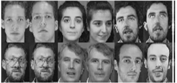
The next experiment is performed using the Yale face database [21], which contains 165 images of 15 indi- viduals (each person has 11 different images) under various facial expressions and lighting conditions. Each image is manually cropped and resized 92 × 112 pixel in this experiment. We use a number of training images between 3 to 10 and the remaining images for test and we take three cases with different input and find the mean of these three cases. From the experimental results listed in Table 3, we can see that the recognition rate of WSD- 2DDA is superior to other methods. Example of images is shown in (Figure 2).
6. Conclusions
A novel feature extraction method, weighted scatter dif- ference (WSD2DDA) is proposed in this paper. This method gives an alternative better solution of the singu- larity problem and reduces the cost in the complexity of the LDA algorithm.
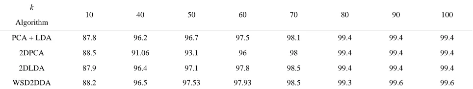
5.3. Experiment on the Headpose Database
The head pose database [22,23] is a benchmark of 2790 monocular face images of 15 persons with variations of pan and tilt angles from –90 to +90 degrees. For every person, 2 series of 93 images (93 different poses) are available. The purpose of having 2 series per person is to
on the size of the face images and the number of classes, the method is very effective in face recognition. The faces used during experimentation are ORL, Yale B and Head Pose face databases respectively on which we demonstrate that the proposed method gives a good per- formance of face recognition rate.
[image:6.595.138.527.86.253.2]Figure 2. Examples of Yale B database. Figure 3. A small sample of head pose database.
Table 2. Recognition time on ORL database per second.
k
Algorithm 3 4 5 6 7 8 9
PCA + LDA 7.67 8.46 10.69 9.72 9.92 9.47 7
2DPCA 7 7.4 7 7.6 7 5.5 4
2DLDA 4 4.5 5 5 4.59 4.22 3.98
[image:6.595.54.538.290.385.2]WSD2DDA 5.41 5.75 5.45 5.42 4.73 4.33 4
Table 3. Comparison result of recognition accuracy on Yale B database.
k
Algorithm 3 4 5 6 7 8 9 10
PCA + LDA 83.22 89.26 95.86 92.89 95 98.51 97.78 97.78
2DPCA 83.38 89.89 96.24 96 95.56 98.51 97.78 97.78
2DLDA 90.5 90.51 95.51 94.67 96.11 99.24 97.78 100
WSD2DDA 93.45 92.51 98.13 98.22 98.33 99.24 98.89 100
Table 4. Chow pan and tilt angles of head pose database.
Negative values Positive values
Pan angel Bottom Top
Tilt angel Left Right
[image:6.595.63.540.413.508.2]Pan (Vertical angle) {–90, –75, –60, –45, –30, –15, 0, +15, +30, +45, +60, +75, +90} Tilt (Horizontal angle) {–90, –60, –30, –15, 0, +15, +30, +60, +90}
Table 5. Comparison result of recognition accuracy on head pose database.
k
Algorithm
10 40 50 60 70 80 90 100
PCA + LDA 87.8 96.2 96.7 97.5 98.1 99.4 99.4 99.4
2DPCA 88.5 91.06 93.1 96 98 99.4 99.4 99.4 2DLDA 87.9 96.4 97.1 97.8 98.5 99.4 99.4 99.4
[image:6.595.57.539.642.733.2]7. Future Work
In the future work we plan to apply Kernel Relevance Weighted (2DLDA) and Kernel Weighted Scatter-Dif- ference Based Two Dimensional Discriminant Analysis for Face Recognition.
REFERENCES
[1] R. O. Dudo, P. E. Hart and D. Stork, “Pattern Classifica-tion,” Wiley, New York, 2000.
[2] K. Fukunage, “Introduction to Statistical Pattren Classi- fication,” Academic Press, San Diego, 1990.
[3] P. N. Belhumeour, J. P. Hespanha and D. J. Kriegman. “Eiegnfaces vs Fisherfaces: Recognition Using Class Spe- cific Linear Projection,” IEEE Transactions on Pattern
Analysis and Machine Intelligence, Vol. 19, No. 7, 1997, pp. 711-720.doi:10.1109/34.598228
[4] D. L. Swets and J. Y. Weng, “Using Discriminant Eigen- features for Image Retrieval,” IEEE Transaction on Pat-
tern Analysis and Machine Intelligence, Vol. 18, No. 8, 1996, pp. 831-836.
[5] S. Dudoit, J. Fridlyand and T. P. Speed, “Comparison of Discrimination Methods for the Classification of Tumors Using Gene Expression Data,” Journal of the American
Statistical Association, Vol. 97, No. 457, 2002, pp. 77-87. doi:10.1198/016214502753479248
[6] W. J. Krzanowski, P. Jonathan, W. V. McCarthy and M. R. Thomas, “Discriminant Analysis with Singular Co- variance Matrices: Methods and Applications to Spectro- scopic Data,” Applied Statistics, Vol. 44, No. 1, 1995, pp. 101-115.doi:10.2307/2986198
[7] X. Li, “Weighted Maximum Scatter Difference Based Feature Extraction and Its Application to Face Recogni- tion,” Machine Vision and Applications, Vol. 22, No. 3, 2011, pp. 591-595.
[8] J. Yang and D. Zhang, “Two-Dimensional PCA: A New Approach to Appearance-Based Face Representation and Recognition,” IEEE Transactions on Pattern Analysis
and Machine Intelligence, Vol. 26, No. 1, 2004, pp. 131- 137.doi:10.1109/TPAMI.2004.1261097
[9] J. Yang and J. Y. Yang, “Form Image Vector to Matrix: A Straightforward Image Projection Technique-IMPCA vs PCA,” Pattern Recognition, Vol. 35, No. 9, 2002, pp. 1997-1999.doi:10.1016/S0031-3203(02)00040-7
[10] J. Ye, R. Janardan and Q. Li, “Two Dimensional Linear Discriminant Analysis,” Proceedings Neural Information
Processing Systems (NIPS), 2004, pp. 1569-1576. [11] J. Ye, “Generalized Low Rank Approximations of Matri-
ces,” The Twenty-First International Conference on Ma-
chine Learning, Banff, Vol. 69, 2004, p. 112.
[12] M. Li and B. Yuang, “2D-LDA: A Novel Statistical Lin- ear Discriminant Analysis for Image Matrix,” Pattern Rec-
ognition Letters, Vol. 26, No. 5, 2005, pp. 527-532.
doi:10.1016/j.patrec.2004.09.007
[13] E. K. Tang, P. N. Suganthan, X. Yao and A. K. Qin, “Lin- ear Dimensionality Reduction Using Relevance Weighted LDA,” Pattern Recognition, Vol. 38, No. 4, 2005, pp. 485-493. doi:10.1016/j.patcog.2004.09.005
[14] K. Chougdali, M. Jedra and N. Zahid, “Kernel Weighted Scatter Difference Discriminant Analysis,” Journal of Image Analysis and Recognition, Vol. 5112, 2008, pp. 977- 983.doi:10.1007/978-3-540-69812-8_97
[15] W. Zhao, A. Krishnaswamy, R. Chellappa, D. L. Swets and J. Weng, “Discriminant Analysis of Principal Com- ponents for Face Recognition-FGR,” International Con-
ference on Automatic Face and Gesture Recognition, 14- 16 April 1998, pp. 336-341.
[16] W. Zhao, R. Chellappa and N. Nandhakumar, “Emprical Performance Analysis of Linear Discriminant, Classifi- ers,” IEEE Computer Society Conference on Computer
Vision and Pattern Recognition, College Park, 23-25 June 1998, pp. 164-169.
[17] W. Zhao, “Subspace Methods in Object/Face Recogni- tion,” International Conference on Neural Networks IEEE, College Park, 1999. pp. 3260-3264.
[18] F. X. Song, D. Zhang, Q. L. Chen and J. Z. Wang, “Face Recognition Based on a Novel Linear Discriminant Crite- rion,” Pattern Analysis and Applications, Vol. 10, No. 3, 2007, pp. 165-174.doi:10.1007/s10044-006-0057-3 [19] S. L. Guan and X. D. Li, “Improved Maximum Scatter
Difference Discriminant Analysis for Face Recognition,”
Proceedings of the 2009 International Workshop on In-
formation Security and Application (IWISA 2009), Qing-dao, 21-22 November 2009.
[20] M. Addlesee, C. Turner and A. Hopper, “Displaying the Future,”4th International Scientific Conference on Work
with Display Units, Milan, October 1994, Technical Re- port 94.13
http://www.cl.cam.ac.uk/research/dtg/attarchive/facedatab ase.html
[21] A. S. Georghiades, P. N. Belhumeur and D. J. Kriegman, “From Few to Many: Illumination Cone Models for Face Recognition under Variable Lighting and Pose,” IEEE
Transactions on Pattern Analysis and Machine Intelli- gence, Vol. 23, No. 6, 2001, pp. 643-660.
http://cvc.yale.edu/projects/yalefacesB/yalefacesB.html
[22] N. Gourier, D. Hall and J. L. Crowley, “Estimating Face Orientation from Robust Detection of Salient Facial Fea- tures.”
http://www-prima.inrialpes.fr/perso/Gourier/Pointing04-Gourier.pdf