Some Penalty-based Constraint Handling Techniques
with Ant Lion Optimizer for Solving Constrained
Optimization Problems
Islam S. Fathi
Department of Mathematics Faculty of Science, ZagazigUniversity
P. O. Box 44519, Zagazig, Egypt
Rasha M. Abo-Bakr
Department of Mathematics Faculty of Science, ZagazigUniversity
P. O. Box 44519, Zagazig, Egypt
R. M. Farouk
Department of Mathematics Faculty of Science, ZagazigUniversity
P. O. Box 44519, Zagazig, Egypt
ABSTRACT
In order to solve constraint optimization problems, constraints should be handled. The most common technique is penalty functions. Ant lion optimizer (ALO) is one of meta-heuristic algorithms which used to solve optimization problems. In this paper, the performance of ALO using different penalty-based methods (static penalty, dynamic penalty, and adaptive penalty) is compared and we make sensitivity analysis of tuning important parameters of penalty methods to show their effects on the performance of the penalty methods; six real engineering problems are used as a benchmark in this paper.
Keywords
Constrained optimization problems, ant lion optimizer, penalty functions, constraint handling.
1.
INTRODUCTION
Optimization problems can be written mathematically as:
(1)
Equation (1) is called unconstrained optimization problem if 0, but if then it is called constrained optimization problem.
Where , is the vector of solution such that , S is the search space defined as n-dimensional bounded space, m is the number of inequality constraint, p is the number of equality constraint, and F
is feasible region which the inequality and equality constraint are satisfied.
Equality constraints are converted into inequality constraint using
(2) is a very small value.
With respect to constraint optimization problems, there are several approaches to handle constrained problem, one of the most popular approach often used is the penalty function [1]. The idea of penalty function is transform constraint optimization problem into an unconstrained problem by adding or subtracting value to the objective function this value called penalty term. There are many methods in penalty function approach to handle constraint problem such as: static penalty, dynamic penalty, adaptive penalty [2]. Each of this method follows general idea of penalty function approach, but the difference between them is the form of the penalty term.
The Ant lion optimizer (ALO) considered one of the latest nature-inspired algorithms which mimic the intelligent behavior of antlion in hunting ants in nature [3]. ALO is one of stochastic optimization (metaheuristic) algorithm that provides very competitive results in unconstrained or constrained optimization problem, using ALO in constrained engineering problem need to appropriate constraint handling method.
This paper compares the performance of different penalty methods for solving constrained optimization problem with ALO.
2.
METHODS OFPENALTY FUNCTION
Penalty function one of constrained handle approaches which proposed by courant in 1940[4]. The main idea of this approach is to convert the constrained problem to unconstrained one through adding or subtracting value to objective function [5].
In general the idea of penalty function can be formulated as For additive way,
(3) Where is penalized function, is objective function and is penalty term. Value of is zero if no violated constraint and positive otherwise.
For multiplicative way,
(4)
Value of is one if no violated constraint and bigger than one otherwise.
In mathematical programming, there are two types of penalty function are used: exterior and interior penalty function. In exterior type, we begins with an infeasible solution and from there we move to the feasible region but in interior type, we begins with an initial point inside the feasible region and the constraint boundaries make the subsequent point generated always lie within the feasible region. One of important drawback of implementation interior penalties is that it needs to begin with an initial feasible solution and it is difficult, so exterior penalties is the most common type used in evolutionary algorithms (ALO) [6].
(5)
Where shows the new objective function to be optimized, and penalty parameter, and the constraint function of and respectively.
The general form of and is
Where and are 1 or 2.
In equation (5) the second term in right side called "penalty term". If the constraint are hold such that and
then will be zero and not effected by penalty term, but if there are violation for constraint such that or , the value of penalty term add to .
The value of penalty term has an important role in getting optimization region. In case of the penalty is too high, algorithm will be pushed inside the feasible region very quickly and not able to explore in the boundary of the feasible region [7, 8]. In case of penalty is too low, algorithm will be spent a lot of search time in exploration of the infeasible region because the penalty will be negligible with respect to the objective function [9] and these is an important issues especially if the optimum of the problem laying on the boundary of the feasible region [10, 11] so the penalty should be kept as low as possible, just above the limit below which infeasible solution are optimal (the minimum penalty rule) [12].
2.1
Static Penalty
In static penalty method the penalty parameter doesn't depend on the current generation of the algorithm that employs the function and remain constant during evolutionary process. In this method optimization process starts with a random population using both feasible and infeasible individuals [13]. In this method we evaluate the individual using
} (6)
Where d is penalty parameter, is the unpenalized objective function, m is the number of constraints.
2.2
Dynamic Penalty
In this method, penalty parameter depends on current generation number. The dynamic function evaluates individuals at each generation t which proposed by Joines and Houck [14] is defined as:
(7) Where c, and are constant determined by the user (c=0.5, = 1 or 2, = 1 or 2) and is defined as:
(8) Where
(9)
(10)
The value of penalty function increase as generation grows. In Joines [10] and Houck approaches, there found that no explanation regarding the sensitivity of the method to different values of , but the quality of the solution is very sensitive to changes in value of and , and the values indicated above for this parameter is good selection, Michalewicz [15] state that this values cause premature convergence in some example. He also state that the method converges either to infeasible solution or solution that is far away from an optimal solution.
2.3
Adaptive Penalty
The method of adaptive penalty depends on updating the penalty parameter at every generation (iteration) according to individual in last generation. In Hadj-Alouane and Bean [16] approach the individual are evaluated by following formula: (11) (11)
Where the penalty parameter is updated at every generation by:
(
Where case#1 indicates that all the best individual in last generation are feasible (i.e. the penalty parameter is decreased), case#2 indicates that all the best individual in last generation are infeasible (i.e. the penalty parameter is increased) and if some of the best individual in last generation are feasible and some infeasible the penalty parameter does not change.
3.
THE ANT LION OPTIMIZER
ALGORITHM
3.1
Main Inspiration
Ant lion algorithm inspired from intelligent behavior of antlion's larvae, where it digs pit in the form of cone using its strong jaw [17] as illustrated in fig.1. Antlion hides in cone waiting for ant or insects to slip on the sand and fall in [18]. The edge of pit is sharp leading to the fall of the prey easily. When prey fall in pit ant lion slide it into the bottom of the pit as illustrated in fig.2. Finally antlion amend the trap to next hunt.
It has been observed that whenever the antlion hungrier whenever the trap bigger and it has the higher chance of catching ant [19].
3.2
Mathematical Formula For The ALO
Ant and Antlion are main elements over search space, ant move to search food and antlion await to hunt it.
Firstly, modeled the position of ant in search space in the following matrix:
Where is matrix of position of each ant over search
space, is position of i-th ant in j-th dimension(variable), n
The fitness value of all ants can be expressed as:
(
Where f( is the matrix for the fitness value for all ants and f is
the objective function.
Besides ant, antlion take position over search space.
Where is the matrix of the position of each antlion over search space, is the position of i-th antlion in j-th
dimension(variable), n shows the number of antlions and m shows the number of dimensions(variables) in space.
The fitness value of all antlions can be expressed as:
Where f ( is the matrix for the fitness value for all antlions and f is the objective function
3.2.1
Ants random wal
k
Since the ants moves randomly in nature when searching for food, This movement is modeled as follows:
[0, cumsum (2r ( -1), cumsum (2r ( -1),., cumsum (2r ( -1)] (12)
Where cumsum indicates the cumulative sum is the
maximum number of iteration, t denotes the current iteration, and r (t) is defined as:
Where rand is random number between 0 and 1
3.2.2
Convergence of Ant towards antlion
When ant trapped in the pit, it sliding towards antlion, ant getting close to antlion, so the boundary of search space decreased adaptively. This may be expressed as:
Where is upper bounded at t-th iteration, is lower bounded at t-th iteration, denotes ratio defined as
, where w is a constant defined as: (w = 2 when t > 0.1 , w = 3when t > 0.5 , w = 4 when t > 0.75 , w = 5 when t > 0.9 , and w=6 when t > 0.95
3.2.3
Ants are affected by antlions’ traps
Each ant affected by traps of antlion either antlion selected by roulette wheel or elite antlion in each iteration.
This affected may be expressed in simple form as:
= (16)
= (17)
Where indicates upper bounded for i-th ant in iteration t, indicates lower bounded for i-th ant in t-th iteration, is upper bounded, is lower bounded, is position of j-th antlion in t-th iteration.
3.2.4
Random walks around elite and selected
antlion
As explained above the better anlion the higher chance of catching ant, roulette wheel used to select the fittest antlion. On the other hand, in each iteration produce the best antlion .so the movement of ant affected by elite antlion and a selected antlion by roulette wheel. Ant walks randomly around and as:
(19)
Where shows position of i-th ant at t-th iteration,
shows the random walk around selected antlion
using roulette wheel at t-th iteration, shows the random
walk around the elite at t-th iteration.
3.2.5
Catching ants
After antlion catch ant and pulls it inside the sand, antlion update their position with corresponding ant. This occurs when fitness of ant is more than fitness of antlion, this expressed as:
Where indicates the position of j-th antlion at t-th
iteration, Where indicates the position of i-th ant at t-th iteration.
4.
NUMERICAL EXPERIMENTS
To evaluate the performance of the ALO algorithm with the different penalty methods mentioned above in solving constraint optimization problems, we conducted experimental study in which six classical engineering problems.
Each of the test problems is solved by ALO, with each of penalty-based methods (static penalty, dynamic penalty, and adaptive penalty) 30 runs over 1000 iterations and the result are reported intables 1-12. Best indicates to the best solution, Ave indicates to the average solution and S.D indicates to standard deviation. The specific parameters of each penalty method are used as following:
In static penalty (d= ).
In dynamic penalty (c=0.5, = 2, = 1).
In adaptive penalty ( .
Test problem 1: Pressure Vessel Design Problem
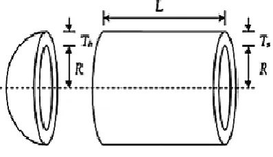
The objective is to minimize the total cost, including the cost of material, forming, and welding. A cylindrical vessel is capped at both ends by hemispherical heads as shown in Figure 1. They are four design variables in this problem: Ts (thickness of the shell), Th (thickness of the head), R (inner
radius), and L (length of the cylindrical section of the vessel). Among the four design variables, Ts and Th are expected to be
integer multiplies of 0.0625 inch, and R and L are continuous variables [20].
Minimize f (x) = 0.6224x1x3x4 + 1.7781x2x32 + 3.1661x12x4 +
19.84x12x3
Subject to: g1(x) = −x1 + 0.0193x3 ≤ 0,
g2(x) = −x2 + 0.00954x3 ≤ 0,
g3(x) = −πx3 2
x4 − (4/3) πx3
3 + 1, 296, 000 ≤ 0,
g4(x) = x4 − 240 ≤ 0.
[image:4.595.327.526.83.197.2]Variable rang: 0 ≤ xi ≤ 100, i = 1, 2, 10 ≤ xi ≤ 200, i = 3, 4.
Fig 1: Pressure Vessel Design Problem
[image:4.595.65.519.321.435.2]This test problem has been solved by ALO algorithm with three penalty-based methods (static penalty, dynamic penalty, and adaptive penalty) and the results represented in tables 1 and 2. The comparison results for this problem show that the adaptive penalty method outperforms on static and dynamic methods in terms of best solution, but dynamic penalty method is outperform in term of Ave and S.D.
Table 1. Compression the best solution for pressure vessel design problem by three penalty-based methods
penalty methods
Static penalty
7.7920E-01 3.8516E-01 4.0373E+01 1.9926E+02 5.8871E+03
Dynamic penalty
7.8064E-01 3.8587E-01 4.0448E+01 1.9823E+02 5.8897E+03
Adaptive penalty
7.7825E-01 3.8469E-01 4.0324E+01 1.9997E+02 5.8859E+03
Table 2. Statistical performance of three penalty-based methods for pressure vessel design problem
Results Static penalty Dynamic penalty Adaptive penalty
Best 5.8871E+03 5.8897E+03 5.8859E+03
Ave 6.7932E+03 6.2888E+03 6.5141E+03
S.D. 2.1554E+03 3.4791E+02 7.4712E+02
Test problem 2: Cantilever Beam Design Problem
The cantilever beam design is made of five elements, each having a hollow cross-section with constant thickness as shown in figure 2. There is a total of 5 structure parameters and also a vertical load applied to the free end of the beam (node 5) and the right side of the beam (node1) is rigidly supported. The aim is to minimize the Weight of the beam. In the final optimal design there is one vertical displacement constraint that should not be violated [21].The mathematical formulation of this problem is as follows:
Minimize f (x) =0.6224( + ),
Subject to: g(x) = ≤ 1,
Variable rang: 0.01 ≤ ≤ 100, Fig 2: cantilever beam Design Problem
[image:4.595.85.529.458.698.2]Table 3. Compression the best solution for cantilever beam design problem by three penalty-based methods
penalty methods
Static penalty 6.016998 5.309663 4.492589 3.501620 2.152792 13.365207 Dynamic penalty 6.020794 5.301333 4.499755 3.499036 2.152790 13.365235 Adaptive penalty 6.008809 5.315777 4.493109 3.502588 2.153413 13.365228
Table 4. Statistical performance of three penalty-based methods for cantilever beam design problem Results Static penalty Dynamic penalty Adaptive penalty
Best 13.365207 13.365235 13.365399
Ave 13.365437 13.365421 13.365399
S.D. 0.000205 0.000173 0.000140
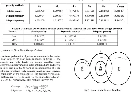
Test problem 3: Gear Train Design Problem
In gear train problem the objective is to minimize the cost of the gear ratio of the gear train as shown in figure 3. The constraints are only limits on design variables (side constraints). Design variables to be optimized are in discrete form since each gear has to have an integral number of teeth. Constrained problems with discrete variables may increase the complexity of the problem [3]. The decision variables of the problem are , , , and which are denoted as ,
, , and , respectively. This problem is given by:
Minimize f (x) = ,
Subject to: 12 ≤ ≤ 60,
Fig 3: Gear train Design Problem
Tables 5 and 6 represent the result of solving this problem by ALO using three penalty-based methods. The adaptive penalty method in obtained the best results from the static and dynamic penalties in best, Ave, S.D.
Table 5. Compression the best solution for Gear train design problem by three penalty-based methods
penalty methods
Static penalty 43.4493 14.9087 12.0095 28.5615 4.0653E-23 Dynamic penalty 43.4493 14.9087 12.0095 28.5615 4.0653E-23 Adaptive penalty 55.1986 38.6950 38.6950 58.3125 3.4239E-25
Table 6. Statistical performance of three penalty-based methods for Gear train design problem
Results Static penalty Dynamic penalty Adaptive penalty
Best 4.0653E-23 4.0653E-23 3.4239E-25
Ave 6.8853E-20 6.8853E-20 5.2360E-20
S.D. 1.1554E-19 1.1554E-19 8.6603E-20
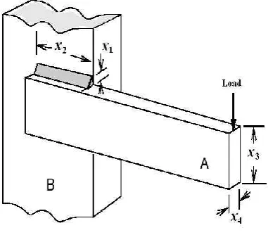
Test problem 4: Welded Beam Design Problem
A welded beam is designed for minimum cost subject to constraint on share stress ( ), buckling load on the bare ( , bending stress in the beam ( end deflection of the beam ( , and side constraints [22], as shown in figure 4 there are four design variable ( ( , the mathematical formulation of this problem is as follows:
Minimize f (x) =
1.10471 0.04811 (14.0+ )
Subject to: g1(x) =
g2(x) =
g3(x) =
g4(x) =0.10471 0.04811 (14.0+ ) 5.0
g5(x) =0.125 g6(x) = g7(x) = p
Where
,
,M ,
R ,
J ,
(1 )
Variable rang: 0 .1≤ xi ≤ 2, i = 1, 4, 0.1 ≤ xi ≤ 10, i = 2, 3.
P 6000 lb, L 4 in, 0.25, E 30 psi, G 12 psi,
[image:6.595.326.517.80.252.2]
Fig 4: Welded Beam Design Problem
In Tables 7 and 8 the results of this problem are represented, it shows that the adaptive penalty methods have better solution in term of best but not better in the terms of Ave, S.D.
Table 7. Compression the best solution for welded beam design problem by three penalty-based methods
penalty methods
Static penalty 0.2054 7.1076 9.0367 0.2057 2.2192
Dynamic penalty 0.2054 7.0702 9.0749 0.2055 2.2203
[image:6.595.305.539.451.686.2]Adaptive penalty 0.2056 7.1006 9.0367 0.2057 2.2187
Table 8. Statistical performance of three penalty-based methods for welded beam design problem Results Static penalty Dynamic penalty Adaptive penalty
Best 2.2192 2.2203 2.2187
Ave 2.3010 2.3231 2.3251
S.D. 0.0748 0.0925 0.0910
Test problem 5: Three-Bar Truss Design Problem
In a three-bar truss problem the objective is to minimize its weight [3]. The structural design problem has a large number of constraints and the objective function is very simple. The constraints here are stress, deflection, and buckling constraints as shown in figure 5.
The mathematical formulation of this problem is as follows: Minimize ) ,
Subject to: g1(x)
g2(x) g3(x)
Variable rang: 0 ,
[image:6.595.55.261.607.709.2]Where kN/c , kN/c
Fig 5: Three-Bar Truss Design Problem
Table 9. Compression the best solution for three-bar truss design problem by three penalty-based methods
Table 10. Statistical performance of three penalty-based methods for three-bar truss design problem
Results Static penalty Dynamic penalty Adaptive penalty
Best 263.89584 263.89584 263.89585
Ave 263.89629 263.89629 263.89617
S.D. 0.0006397 0.0007456 0.0003781
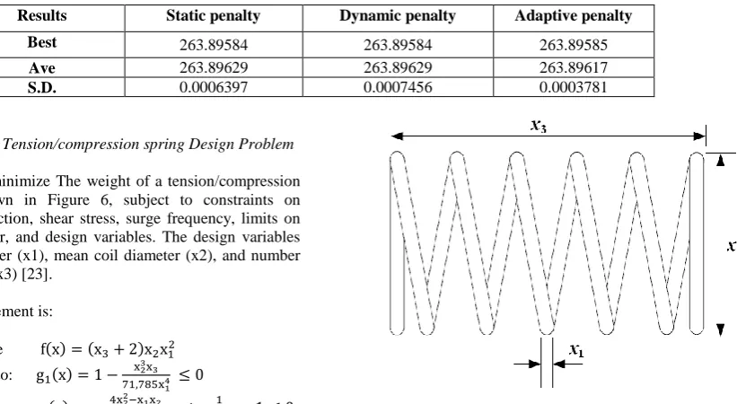
Test problem 6: Tension/compression spring Design Problem This problem minimize The weight of a tension/compression spring as shown in Figure 6, subject to constraints on minimum deflection, shear stress, surge frequency, limits on outside diameter, and design variables. The design variables are wire diameter (x1), mean coil diameter (x2), and number of active coils (x3) [23].
The formal statement is:
Minimize Subject to:
Variable rang:
Fig 6: Tension/compression spring Design Problem
[image:7.595.85.508.545.640.2]Tension/compression spring Design problem is solved by ALO with each of penalty-based methods; the results of the best solution and Statistical performance which represented in tables 11and 12 indicates that the adaptive penalty method is obtained the best result from static and dynamic in best term and dynamic penalty have better solutions in Ave and S.D.
Table 11. Compression the best solution for Tension/compression spring design problem by three penalty-based methods
penalty methods
Static penalty 0.0514103 0.3500494 11.690909 0.012666
Dynamic penalty 0.0520775 0.3661357 10.757475 0.012668
[image:7.595.100.494.664.722.2]Adaptive penalty 0.0518434 0.3604415 11.073951 0.012665
Table 12. Statistical performance of three penalty-based methods for Tension/compression spring design problem
Results
Static penalty Dynamic penalty Adaptive penalty
Best
0.012667 0.012668 0.012666
Ave
0.013669 0.013450 0.013600S.D. 0.001613 0.001341 0.001726
penalty methods
The convergence curves of ALO with static, dynamic and adaptive penalties on engineering problems are illustrated in Fig 7.
5.
ANALYSIS OF PARAMETER
VALUES FOR PENALTY METHODS
In this section, we have provided sensitively analysis for the parameter of penalty methods and its effects the performance of results of test problems. The static and adaptive penalties are implemented but in dynamic penalty parameter t dependent on current generation number (iteration).
5.1
Static Penalty
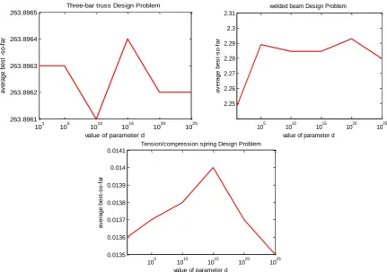
In Static penalty we study the effects of parameter d on the average value of test problems, the comparative results of the average value of 10 runs are illustrated in table 13 and figure 8.
Table13 and Figure 8 shows that the average values sometimes improves and sometimes worsen with the increase of parameter d.
5.2
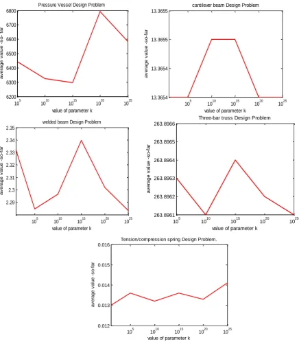
Adaptive Penalty
In the adaptive penalty, we study k (1) the initial value of parameter and its effects on the average value, result of the average value of 10 runs are presented in table 14 and figure 9 indicates that also the average value sometimes improve and sometimes worsen with the increase of parameter k (1), so in each penalty method, some appropriate values of penalty parameters should be selected.
200 400 600 800 1000
104 Pressure Vessel Design Problem
Iteration B e st sco re o b ta in e d so f a r static dynamic adaptive
200 400 600 800 1000
100.4 100.5 100.6 100.7
welded beam Design Problem
Iteration B e s t s c o re o b ta in e d s o f a r static dynamic adaptive
100 200 300 400 500 600 700 800 900 1000 100.35
100.36 100.37
welded beam Design Problem
Iteration B e st sco re o b ta in e d so f a r static dynamic adaptive
200 400 600 800 1000
101.2 101.4 101.6 101.8
cantilever beam Design Problem
Iteration B e s t s c o re o b ta in e d s o f a r static dynamic adaptive
200 400 600 800 1000
101.12598 101.126 101.12602
cantilever beam Design Problem
Iteration B e st sco re o b ta in e d so f a r static dynamic adaptive
0 200 400 600 800 1000
102.422 102.424 102.426 102.428 102.43 iteration B e s t s c o re o b ta in e d s o f a r
Three-bar truss Design Problem
Fig.7: Convergence curves of ALO with static, dynamic and adaptive penalties on the test problems
0 200 400 600 800 1000
iteration
B
e
st
sco
re
o
b
ta
in
e
d
so
f
a
r Three-bar truss Design Problem
static dynamic adaptive
0 200 400 600 800 1000
10-5 100 105 1010
iteration
B
es
t
sc
or
e
ob
ta
in
ed
s
o
fa
r
Tension/compression spring Design Problem
static dynamic adaptive
0 200 400 600 800 1000
10-1.91 10-1.82
iteration
B
e
st
sco
re
o
b
ta
in
e
d
so
f
a
r Tension/compression spring Design Problem
static dynamic adaptive
105 1010 1015 1020 1025
6300 6400 6500 6600 6700 6800 6900
value of parameter d
a
v
e
ra
g
e
v
a
lu
e
-s
o
-f
a
r
Pressure Vessel Design Problem
105 1010 1015 1020 1025
13.3653 13.3653 13.3654 13.3654 13.3655 13.3655
value of parameter d
a
v
e
ra
g
e
b
e
s
t-s
o
-f
a
r
Fig 8: effects of change value of parameter d on the average best value for test problems
Table 13. Results of test problems with different values of parameter d in static penalty
Pressure Vessel Design Problem
cantilever beam Design Problem
welded beam Design Problem
Three-bar truss Design Problem
Tension/compression spring Design Problem
10 infeasible 13.3653 2.2483 263.8963 0.0136
6.3225e+003 13.3654 2.2889 263.8963 0.0138
6.3774e+003 13.3655 2.2844 263.8961 0.0137
6.4055e+003 13.3655 2.2844 263.8964 0.0140
6.8926e+003 13.3654 2.2927 263.8962 0.0137
6.5939e+003 13.3655 2.2796 263.8962 0.0135
101 105 1010 1015 1020 1025
263.8961 263.8962 263.8963 263.8964 263.8965
value of parameter d
a
v
e
ra
g
e
b
e
s
t
-s
o
-f
a
r
Three-bar truss Design Problem
105 1010 1015 1020 1025
2.25 2.26 2.27 2.28 2.29 2.3 2.31
value of parameter d
a
v
e
ra
g
e
b
e
s
t-s
o
-f
a
r
welded beam Design Problem
105 1010 1015 1020 1025
0.0135 0.0136 0.0137 0.0138 0.0139 0.014 0.0141
value of parameter d
a
v
e
ra
g
e
b
e
s
t-s
o
-f
a
r
Fig 9: effects of change value of parameter k (1) on the average best value for test problems
Table 14. Results of test problems with different values of parameter k(1) in adaptive penalty
Design Problem Pressure Vessel
cantilever beam Design Problem welded beam Design Problem Three-bar truss Design Problem Tension/compression spring Design Problem.
10 infeasible 13.3654 2.3320 infeasible 0.0130
6.4414e+003 13.3654 2.2845 263.8963 0.0136
6.3254e+003 13.3655 2.2965 263.8961 0.0132
6.2965e+003 13.3655 2.3397 263.8964 0.0136
6.7917e+003 13.3654 2.3018 263.8962 0.0133
6.5837e+003 13.3654 2.2832 263.8961 0.0141
105 1010 1015 1020 1025
6200 6300 6400 6500 6600 6700 6800
value of parameter k
a v e ra g e v a lu e -s o - fa r
Pressure Vessel Design Problem
105 1010 1015 1020 1025 13.3654
13.3654 13.3655 13.3655
value of parameter k
a v e ra g e v a lu e -s o -f a r
cantilever beam Design Problem
105 1010 1015 1020 1025 2.29 2.3 2.31 2.32 2.33 2.34 2.35
value of parameter k
a v e ra g e v a lu e -s o -f a r
welded beam Design Problem
105 1010 1015 1020 1025
263.8961 263.8962 263.8963 263.8964 263.8965 263.8966
value of parameter k
a v e ra g e v a lu e -s o -f a r
Three-bar truss Design Problem
105 1010 1015 1020 1025
0.012 0.013 0.014 0.015 0.016
value of parameter k
a v e ra g e v a lu e -s o -f a r
6. CONCLUSION
In order to solve the constrained optimization problems, the constraints should be handled. There are most of constraints handling techniques have been suggested. The most popular constraint handling technique among user is penalty function. In this paper, results are discussed in two ways. Firstly, we have studied the performance of the Ant Lion Optimizer (ALO) with a number of penalty-based methods (static, dynamic and adaptive penalty). A small comparative study is conducted using six real engineering problems as benchmark. Experimental results show that the methods of adaptive penalty is outperform on the static and dynamic methods in most of engineering problems, this due to that the penalty parameter doesn't remain constant but updates itself at every generation (iteration) during evolutionary process, but in general it is impossible to say one of the methods is the best for every problem.
Secondly, sensitivity analysis of choosing parameters of static and adaptive penalty methods is performed to check the performance of ALO. The obtained results show that the best value obtained with 30 runs sometimes improve and sometimes worsen with fine-tuning of the parameters and the main problem is to set appropriate values of the penalty parameters so the users have to experiment with different values of penalty parameters.
There is several research directions can be recommended for future work such as investigated the performance of ALO in other benchmark and real-life problems. Another research direction is to use other different constraints handling techniques.
7. ACKNOWLEDGMENTS
First of all, I would like to express my sincere gratitude to Allah - the Most Gracious, the Most Merciful for wonderful opportunity who has given me to pursue and complete my work.
I wish to thank all the people who made this work possible. I would like to thank my supervisors, Prof. Dr. Roushdi Mohamed Farouk and Dr. Rasha Mohamed abobakr for their time and cooperation in reviewing this work.
Finally, I would like to thank my father, mother, brothers and wife for their love, trust, understanding, and every kind of support not only throughout my work but also throughout my life.
8. REFERENCES
[1] Thomas Philip Runarsson, and Xin Yao. Stochastic Ranking for for Constrained Evolutionary Optimization. IEEE Transactions on Evolutionary Computation, 2000. [2] Michalewicz, Z. and Schouenauer, M. Evolutionary
algorithms for constrained parameter optimization problem, Evolutionary Computation, 4, 1-32, 1996. [3] Mirjalili S. A., The Ant lion optimizer, Advance in
Engineering software vol. 83, pp.80-90, (2015).
[4] R.Courant, variational methods for the solution of problems of equilibrium and vibration, Bull. Am. Math. Soc. 49(1943) 1-23.
[5] Carlos A. Coello Coello. Theoretical and numerical constraint-handling techniques used with evolutionary algorithms: a survey of the state of the art. Comput. Methods Appl. Mech. Engrg. 191(2002) 1245-1287.
[6] ¨Ozg¨ur Yeniay. PENALTY FUNCTION METHODS FOR CONSTRAINED OPTIMIZATION WITH GENETIC ALGORITHMS. Mathematical and Computational Applications, Vol. 10, NO. 1, PP. 45-56, 2005.
[7] R.G. Le Riche, R.T. Haftka, Optimization of laminate stacking sequence for buckling load maximization by genetic algorithm, AIAA J. 31 (5) (1993) 951-970. [8] R.G Le Riche, C. Knopf-lenoir, R.T. Haftka, A segregated
genetic algorithm for constrained structural optimization, in: L.J. Eshelman (Ed.) proceedings of the Sixth International Conference on Genetic Algorithms, University of Pittsburgh, Morgan Kaufmann, San Mateo, CA, July 1995, pp. 558-565.
[9] A.E. Smith, D.W. Coit, Constraint handling techniques – penalty function, in: T. B¨ack, D.B. Fogel, z. Michalewicz (Eds.), Handbook of Evolutionary Computation, Oxford University Press and Institute of Phsics Publishing, 1997 (Chapter C 5.2).
[10]W. Siedecki, J. Sklanski, Constrained genetic optimization via dynamic reward-penalty balancing and its use in pattern recognition, in: J.D. Schaffer (Ed.), proceedings of the Third International Conference on Genetic Algorithms, George Mason University, Morgan Kaufmann, San Mateo, CA, June 1989, pp. 141-150. [11]A.E. Smith, D.M. Tate, Genetic optimization using a
penalty function, in: S.Forrest(Ed.), proceedings of the Fifth International Conference on Genetic Algorithms, University of Illinois at Urbana-Champaign, Morgan Kaufmann, San Mateo, CA, July 1993, pp. 499-503. [12]L. Davis, Genetic Algorithms and Simulated Annealing,
Pitman, London, 1987.
[13]Homaifar, A., Lai, S.H.Y. and Qi, X. Constrained optimization Via genetic algorithms, Simulation, 62, 242-254, 1994.
[14]Joines, J. and Houk, C. On the use of non-stationary penalty functions to solve non-linear constrained otimization problems with Gas, Proceedings of the First IEEE International Conference on Evolutionary Computation, IEEE Press, 579-584, 1994.
[15]Z. Michalewicz, G. Nazhiyath, Genocop III: A co-evolutionary algorithm for numerical optimization with nonlinear constraints, in : D.B. Fogel (Ed.) proceedings of the Second IEEE International Conference on Evolutionary Computation, IEEE press, piscataway, NJ, 1995, pp. 647-651.
[16]Hadj-Alouane, A.B. and Bean, J.C. A Genetic algorithm for the multiple-choice inter program, Operations Research, 45, 92-101, 1997.
[17]Scharf I, Subach A, Ovadia O.Foraging behviour and habitat selection in Pit-building antlion larvae in constant light or dark conditions. Anim Behav 2008;76:2049-57. [18]Scharf I, Ovadia O. Factors influencing site abandonment
and site selection in a sit-and-wait predator: a review of pit-building antlion larvae. J Insect Behav 2006;19:197-218.
[20]B.k. kannan, S.N. Kramer, An augmented Lagrange multiplier based method for mixed integer discrete continuous optimization and its applications to mechanical design, J. Mech. Des. Trans. ASME 116 (1994) 318-320. [21]Chickermane H, Gea H. Structural optimization using a
New local approximation method. Int J Numer Meth Eng 1996;39:829-46.
[22]S.S. Rao, Engineering Optimization, third ed., Wiley, New York, 1996.