Improvised Priority based Round Robin CPU Scheduling

Improvised Priority based Round Robin CPU Scheduling

Kawser Irom Rushee

Department of Computer

Science

American International

University-Bangladesh

Dhaka, Bangladesh

Kazi A. Kalpoma

Department of Computer

Science and Engineering

Ahsanullah University of

Science & Technology

Dhaka, Bangladesh

Tahmina Akter

Department of Computer

Science

American International

University-Bangladesh

Dhaka, Bangladesh

ABSTRACT

In this paper a new approach for Priority based round robin CPU scheduling algorithm is performed which improves the CPU performance in real time operating system. It retains the advantage of existing round-robin algorithms [5, 6, 8] and improves the performance. The proposed algorithm gives better performance with given priority as well as assigned priority and in both cases, minimize average waiting time which context switch number, and Average turnaround time from existing round robin algorithms. The paper gives a Graph comparative analysis of proposed algorithm with existing round robin scheduling algorithms on various cases with different combination of CPU burst varying time quantum, average waiting time, average turnaround time and number of context switches.

General Terms

Algorithms, CPU performance

Keywords

Round-Robin, Context switch number, Average waiting time, Average turnaround time

1.

INTRODUCTION

The process scheduling is the activity of the process manager that manages the deletion of the running process from the CPU and the choice of another process on the basis of a specific approach. Process scheduling is an essential part of a Multiprogramming operating system [9]. Multiple processes are permitted by the operating system to be loaded into the executable memory at a time and loaded process shares the CPU using time multiplexing CPU scheduling decides which processes run when there are more than one process running. It is important because it can have a big effect on resource utilization and the overall performance of the system. There is a bunch of CPU scheduling algorithms [1, 2] like

•First Come First Serve (FCFS) •Shortest Job First Scheduling (SJFS) •Round Robin scheduling (RR) •Priority Scheduling etc

But except Round Robin scheduling these are rarely used because of their drawbacks and disadvantages.

A number of assumptions are considered in CPU scheduling which are as follows [3, 4] :

1. Job pool consists of runnable processes waiting for the CPU.

2. All processes are self-determining and race for resources.

3. The job of the scheduler is to distribute the limited resources of CPU to the different processes fairly and in a way that optimizes some performance criteria.

Schedulers are superior system software which handles process scheduling in numerous ways. Their main task is to select the jobs to be submitted into the system and to decide which process to run [10]. Schedulers are of three types •Long Term Scheduler

•Short Term Scheduler •Medium Term Scheduler Priority based problem (PB):

1. Ishwari and Deepa [6] in PB algorithm they used prioritization only once when round robin algorithm is applied. Then they sort rest process according the shortest burst time and give a new priority according that sequence. However the problems are:

a. If a new process comes with high priority and big burst time, according PB algorithm this new process priority will change lowest priority because of its big burst time.

b. Similarly if a new process comes with low priority and small burst time, according this algorithm this new process priority will change to higher priority because of its small burst time.

2. Starvation of big burst time is possible if small no of burst time processes keep arriving continuously.

Improvised RR problem (RR):

Abhishek et al. [5] did not use any priority. Sorted the processes according to small burst time they used round robin algorithm. But if a process with big burst time arrives which is most important than other small no of burst time process then it has to wait until other processes given time quantum is over. A superior scheduling algorithm for real time and time sharing system must have the following characteristics [7]: � Minimum context switches.

� Maximum CPU utilization. � Maximum throughput. � Minimum turnaround time. � Minimum waiting time.

International Journal of Computer Applications (0975 – 8887) Volume 179 – No.32, April 2018

algorithms that shows our algorithm is successful to achieve our objective.

2.

Proposed Algorithm

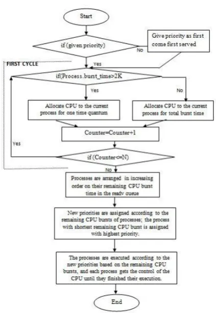
We have modified the Priority based round robin CPU scheduling algorithm to improve the performance of CPU. Proposed algorithm is described below with different steps and a flowchart is given in Figure 1. In this algorithm, if processes come without given priority, a priority is assigned as FCFS basis first. Initially Counter (Counts Number of process) is initialized as 1 and it increase up to N (total number of process). Before performing the algorithm it needs to calculate the shortest and largest burst time to decide quantum time, K. Following condition is considered for quantum time, K:

Shortest burst_time ≤ K ≤ 0.5(Largest burst_time) .

Figure 1: Flow chart of our proposed algorithm

Proposed algorithm consists following three steps:

Step1: if Priority is given move to step2 else give priority based on FCFS and then move to step 2

Step 2: Allocate CPU to every process in round robin fashion, according to the priority, for given time quantum (K) considering the following logic which impose only for the first cycle. Move to step 3 after completion of first cycle. if(process.burst_time>2K)

Then allocate CPU to the current process for one time quantum

Else

Allocate CPU to the current process for total burst time Step 3: After completion of Second step following steps are performed:

a) Processes are arranged in increasing order on their remaining CPU burst time in the ready queue. New priorities are given according to the remaining CPU bursts of processes; the process with shortest remaining CPU burst is allocated with highest priority.

b) The processes are executed according to the new priorities based on the remaining CPU bursts, and each process gets the control of the CPU until they finished their execution. We have taken various cases with variation in burst time to evaluate the performance. Our algorithm performs better in each case which has been shown in the next section. An example has been shown below to illustrate our algorithm. In Table 1 process with burst time and given priority is shown. For better understanding we have sort the processes according to priority also in this table.

Table 1: Processes with burst time, priority and after Sort according to Priority

Given After Sort

Process Burst time

Priority (Given)

Process Burst time

Priority (Given)

A 22 4 C 9 1

B 18 2 B 18 2

C 9 1 D 10 3

D 10 3 A 22 4

E 4 5 E 4 5

First sort the processes according to priority.

Table 2: Expected CPU burst for 2nd and 3rd Step

2nd Step 3rd Step

Proces Burst time

Priority

(Given) Process Burst

time

Priority (Assigned)

C 9 1 B 13 1

B 5 2 A 17 2

D 10 3

A 5 4

E 4 5

In step 1, in this case priority is given. So, we have to move to step 2.

In step 2, Let time quantum=5ms

Largest burst_time = 22 Since, 4 < K < 11

Here Process C has burst time 9 and 9 is not greater than 2*time quantum. So we have to allocate CPU for process C according to its burst time.

In the same manner other processes are executed according to their priorities. The sequence of execution for step2 is shown in Table 2. Expected CPU burst for 2nd step is shown in Table 2.

Step 3 includes the changing of process’s priorities according to the remaining CPU Burst Time. The process with least remaining CPU Burst Time is assigned highest priority. The new assigned priorities and Expected CPU burst for 3rd step is also shown in Table 2.

Now the processes are executed according to the new priority allocated without taking consideration of time quantum. The Gantt chart of the process execution by our algorithm is given in Figure 2.

0 9 14 24 29 33 46 63 Figure 2: Gantt chart

Result:

Context Switch: 6 Average waiting time: 22.4 Average turnaround Time: 35

3.

Comparison with Existing algorithms

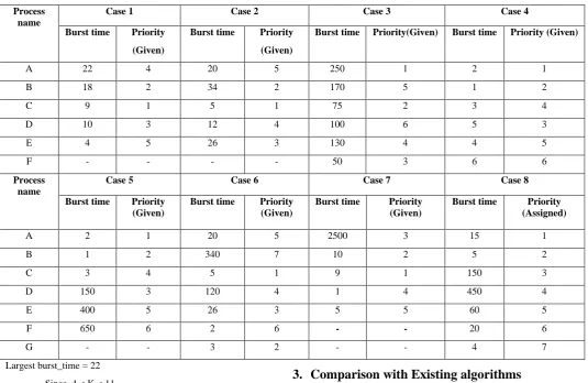
In this section proposed algorithm is compared with existing round-robin algorithms for different cases. These comparisons take processes with different combination of burst time, priority and varying different time quantum. Proposed algorithm is compared with existing round-robin algorithms which are Round Robin without Priority (RRWP), Round Robin with Priority (RRP), Improvised Round Robin (IRR). We compared our proposed algorithm with these three algorithms for about 50 times in different types of cases including all small burst time process, all large burst time process, and all medium burst time process and taking different combination of them. Eight of the cases are shown in Table 3. For each case minimum three different time quantum has been taken. So more than 24 numbers of comparisons have been shown here. Comparisons have been made for average waiting time, average context switch and average turnaround time. Comparison results are shown in Table 4 to Table 11.

Table 4: Comparison of algorithms for case1

Algorith m

Averag e Waiting

Time

Average Turnaroun

d Time

Contex t Switch

Time Quantu

m

(K)

RRWP 33.2 45.8 13

5

RRP 29.2 41.8 13

IRR 26.2 38.8 8

Process name

Case 1 Case 2 Case 3 Case 4

Burst time Priority

(Given)

Burst time Priority

(Given)

Burst time Priority(Given) Burst time Priority (Given)

A 22 4 20 5 250 1 2 1

B 18 2 34 2 170 5 1 2

C 9 1 5 1 75 2 3 4

D 10 3 12 4 100 6 5 3

E 4 5 26 3 130 4 4 5

F - - - - 50 3 6 6

Process name

Case 5 Case 6 Case 7 Case 8

Burst time Priority (Given)

Burst time Priority (Given)

Burst time Priority (Given)

Burst time Priority (Assigned)

A 2 1 20 5 2500 3 15 1

B 1 2 340 7 10 2 5 2

C 3 4 5 1 9 1 150 3

D 150 3 120 4 1 4 450 4

E 400 5 26 3 5 5 60 5

F 650 6 2 6 - - 20 6

G - - 3 2 - - 4 7

International Journal of Computer Applications (0975 – 8887) Volume 179 – No.32, April 2018

Proposed 22.4 35 6

RRWP 36.8 49.4 8

9

RRP 29.6 42.2 8

IRR 28 40.6 7

Proposed 24.6 37.2 5

RRWP 36 48.6 6

12

RRP 28 40.6 6

IRR 28 40.6 6

Proposed 26.4 39 4

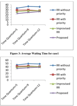
Graph representation of average waiting time, average turnaround time and context switch for case 1 are given below in Figure 3, Figure 4 and Figure 5 respectively.

Figure 3: Average Waiting Time for case1

Figure 4: Average Turnaround Time for case1

Figure 5: Context Switch for case1

Table 5: Comparison of algorithms for case2

Algorithm Average Waiting Time

Average Turnaround

Time

Context Switch

Time Quantum

(K)

RRWP 46.4 65.8 20

5

RRP 46.4 65.8 20

IRR 30.4 49.8 8

Proposed 30.4 49.8 8

RRWP 48 67.4 11

10

RRP 48.8 67.8 11

IRR 36.4 55.8 8

Proposed 34.4 53.8 6

RRWP 48.4 67.8 8

15

RRP 46.6 66 8

IRR 39.4 58.8 7

Proposed 37.4 56.8 5

RRWP 52.6 72 7

19

RRP 49 68.4 7

IRR 43.4 62.8 7

Proposed 37.2 56.6 4

Graph representation of average waiting time, average turnaround time and context switch for case 2 are given below in Figure 6, Figure 7 and Figure 8 respectively.

0

5

10

15

20

25

30

35

40

RR without

priority

RR with

priority

Improvised

RR

Proposed

0

10

20

30

40

50

60

RR without

priority

RR with

priority

Improvised

RR

Proposed

0

2

4

6

8

10

12

14

RR without

priority

RR with

priority

Improvised

RR

Figure 6: Average Waiting Time for case2

Figure 7: Average Turnaround Time for case2

Figure 8: Context Switch for case2

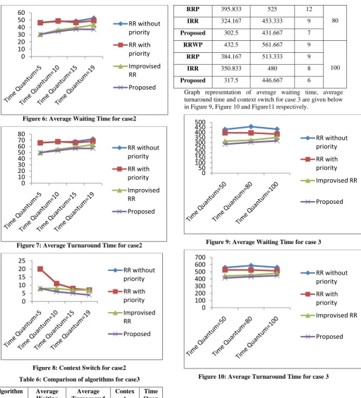
Table 6: Comparison of algorithms for case3

Algorithm Average Waiting Time

Average Turnaround

Time

Contex t Switch

Time Quan tum

(K)

RRWP 430 559.167 16

50

RRP 396.667 525.833 16

IRR 313.333 442.5 10

Proposed 284.167 413.333 8

RRWP 457.5 586.667 12

RRP 395.833 525 12

80

IRR 324.167 453.333 9

Proposed 302.5 431.667 7

RRWP 432.5 561.667 9

100

RRP 384.167 513.333 9

IRR 350.833 480 8

Proposed 317.5 446.667 6

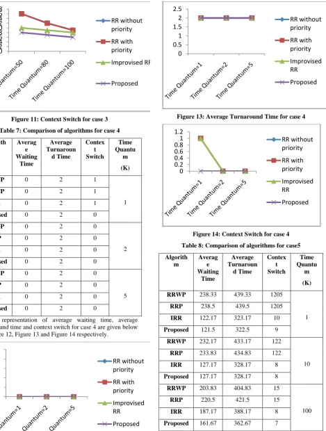
Graph representation of average waiting time, average turnaround time and context switch for case 3 are given below in Figure 9, Figure 10 and Figure11 respectively.

Figure 9: Average Waiting Time for case 3

Figure 10: Average Turnaround Time for case 3

0

10

20

30

40

50

60

RR without

priority

RR with

priority

Improvised

RR

Proposed

0

10

20

30

40

50

60

70

80

RR without

priority

RR with

priority

Improvised

RR

Proposed

0

5

10

15

20

25

RR without

priority

RR with

priority

Improvised

RR

Proposed

0

50

100

150

200

250

300

350

400

450

500

RR without

priority

RR with

priority

Improvised RR

Proposed

0

100

200

300

400

500

600

700

RR without

priority

RR with

priority

Improvised RR

International Journal of Computer Applications (0975 – 8887) Volume 179 – No.32, April 2018

Figure 11: Context Switch for case 3

Table 7: Comparison of algorithms for case 4

Algorith m

Averag e Waiting

Time

Average Turnaroun

d Time

Contex t Switch

Time Quantu

m

(K)

RRWP 0 2 1

1

RRWP 0 2 1

IRR 0 2 1

Proposed 0 2 0

RRWP 0 2 0

2

RRP 0 2 0

IRR 0 2 0

Proposed 0 2 0

RRWP 0 2 0

5

RRP 0 2 0

IRR 0 2 0

Proposed 0 2 0

Graph representation of average waiting time, average turnaround time and context switch for case 4 are given below in Figure 12, Figure 13 and Figure 14 respectively.

Figure 12: Average Waiting Time for case 4

Figure 13: Average Turnaround Time for case 4

Figure 14: Context Switch for case 4

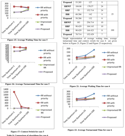
Table 8: Comparison of algorithms for case5

Algorith m

Averag e Waiting

Time

Average Turnaroun

d Time

Contex t Switch

Time Quantu

m

(K)

RRWP 238.33 439.33 1205

1

RRP 238.5 439.5 1205

IRR 122.17 323.17 10

Proposed 121.5 322.5 9

RRWP 232.17 433.17 122

10 RRP 233.83 434.83 122

IRR 127.17 328.17 8

Proposed 127.17 328.17 8

RRWP 203.83 404.83 15

100

RRP 220.5 421.5 15

IRR 187.17 388.17 8

Proposed 161.67 362.67 7

Graph representation of average waiting time, average turnaround time and context switch for case 5 are given below in Figure 15, Figure 16 and Figure 17 respectively.

0

2

4

6

8

10

12

14

16

18

RR without

priority

RR with

priority

Improvised RR

Proposed

0

0.2

0.4

0.6

0.8

1

RR without

priority

RR with

priority

Improvised

RR

Proposed

0

0.5

1

1.5

2

2.5

RR without

priority

RR with

priority

Improvised

RR

Proposed

0

0.2

0.4

0.6

0.8

1

1.2

RR without

priority

RR with

priority

Improvised

RR

Figure 15: Average Waiting Time for case 5

Figure 16: Average Turnaround Time for case 5

Figure 17: Context Switch for case 5

Table 9: Comparison of algorithms for case 6

Algorith m

Averag e Waiting

Time

Average Turnaroun

d Time

Contex t Switch

Time Quantu

m

(K)

RRWP 84.86 158.57 53

10

RRP 73.57 147.286 53

IRR 53.571 127.286 10

Proposed 53.285 127 9

RRWP 104.86 178.57 24

25

RRP 79 152.714 24

IRR 68.286 142 9

Proposed 58.286 132 8

RRWP 183 256.714 10

100 RRP 90.429 164.143 10

IRR 90.429 164.423 8

Proposed 78.714 152.429 7

Graph representation of average waiting time, average turnaround time and context switch for case 6 are given below in Figure 21, Figure 22 and Figure 23 respectively.

Figure 21: Average Waiting Time for case 6

Figure 22: Average Turnaround Time for case 6

0

50

100

150

200

250

300

RR without

priority

RR with

priority

Improvised

RR

Proposed

0

50

100

150

200

250

300

350

400

450

500

RR without

priority

RR with

priority

Improvised

RR

Proposed

0

200

400

600

800

1000

1200

1400

RR without

priority

RR with

priority

Improvised

RR

Proposed

0

50

100

150

200

RR without

priority

RR with

priority

Improvised RR

Proposed

0

50

100

150

200

250

300

RR without

priority

RR with

priority

Improvised RR

International Journal of Computer Applications (0975 – 8887) Volume 179 – No.32, April 2018

Figure 23: Context Switch for case 6

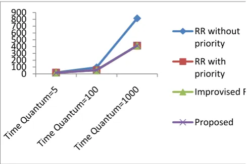
Table 10: Comparison of algorithms for case 7

Algorith m

Averag e Waiting

Time

Average Turnaroun

d Time

Contex t Switch

Time Quantu

m

(K)

RRWP 20.6 525.6 505

5

RRP 18.4 523.4 505

IRR 18.4 523.4 7

Proposed 16.6 521.6 5

RRWP 94.8 599.8 28

100

RRP 54.6 559.6 28

IRR 54.6 559.6 5

Proposed 54.6 559.6 5

RRWP 814.8 1319.8 6

1000

RRP 414.6 919.6 6

IRR 414.6 919.6 5

Proposed 414.6 919.6 5

Graph representation of average waiting time, average turnaround time and context switch for case 7 are given below in Figure 24, Figure 25 and Figure 26 respectively.

Figure 24: Average Waiting Time for case 7

Figure 25: Average Turnaround Time for case 7

Figure 26: Context Switch for case 7

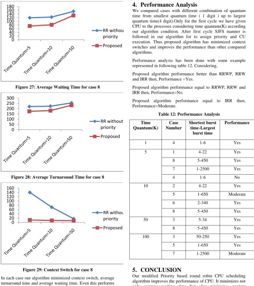
Table 11: Comparison of algorithms for case 8

Algorith m

Averag e Waiting

Time

Average Turnaroun

d Time

Contex t Switch

Time Quantu

m

(K)

RRWP 119.29 219.86 140

5

Proposed 74.29 174.86 11

RRWP 122.86 223.43 71

10

Proposed 81 181.57 9

RRWP 153.86 254.43 17

50 Proposed 131.86 232.43 8

Here, for case 8 priority is not given. So priority is assigned as FCFS manner. That is why in this case comparison has done only with RRWP. Graph representation of average waiting time, average turnaround time and context switch for case 8 are given below in Figure 27, Figure 28 and Figure 29 respectively.

0

10

20

30

40

50

60

RR without

priority

RR with

priority

Improvised RR

Proposed

0

100

200

300

400

500

600

700

800

900

RR without

priority

RR with

priority

Improvised RR

Proposed

0

200

400

600

800

1000

1200

1400

RR without

priority

RR with

priority

Improvised RR

Proposed

0

100

200

300

400

500

600

RR without

priority

RR with

priority

Improvised RR

Figure 27: Average Waiting Time for case 8

Figure 28: Average Turnaround Time for case 8

Figure 29: Context Switch for case 8

In each case our algorithm minimized context switch, average turnaround time and average waiting time. Even this performs better for without given priority processes (for case 8 shown in Table 11). In every comparison our algorithm gives better performance except a very few comparison such as shown in table 5 for quantum time 5 only (Equal performance to IRR and better than RRWP and RRP), table 7 for quantum time 2 ,5 and table 10 for quantum 100 and 1000(Equal performance to IRR and better than RRWP and RRP) . This can be neglected as it gives equal performances on those comparisons. It also performs better than RRWP in the case of without given priority. Provided all comparisons in above proofs that, proposed algorithm gives better performance than RRP, RRWP, and IRR with accuracy.

4.

Performance Analysis

We compared cases with different combination of quantum time from smallest quantum time ( 1 digit ) up to largest quantum time(4 digit).Only for the first cycle we have given CPU to the processes considering time quantum(K) according our algorithm condition. After first cycle SJFS manner is followed in our algorithm for to assign priority and CU execution. Thus proposed algorithm has minimized context switches and improves the performance than other compared algorithms.

Performance analysis has been done with some example represented in following table 12. Considering,

Proposed algorithm performance better than RRWP, RRW and IRR then, Performance =Yes.

Proposed algorithm performance equal to RRWP, RRW and IRR then, Performance=No.

Proposed algorithm performance equal to IRR then, Performance=Moderate.

Table 12: Performance Analysis

Time Quantum(K)

Case Number

Shortest burst time-Largest

burst time

Performance

1 4 1-6 Yes

5 1 4-22 Yes

8 5-450 Yes

7 1-2500 Yes

4 1-6 No

10 2 4-22 Yes

5 1-650 Moderate

6 2-340 Yes

8 5-450 Yes

50 3 5-34 Yes

8 5-450 Yes

100 3 50-250 Yes

5 1-650 Yes

7 1-2500 Moderate

5.

CONCLUSION

Our modified Priority based round robin CPU scheduling algorithm improves the performance of CPU. It minimizes not only average waiting time but also minimizes context switching and average turnaround time. It gives better performance for both cases with given priority and without given priority processes.

In future, it can be possible to improve the algorithm for the cases only where the performance of proposed algorithm is equal rather than better.

6.

REFERENCES

[1] Silberschatz, A., Peterson, J. L., and Galvin, B.,Operating System Concepts, Addison Wesley, 7th Edition, 2006.

0

20

40

60

80

100

120

140

160

180

RR without

priority

Proposed

0

50

100

150

200

250

300

RR without

priority

Proposed

0

20

40

60

80

100

120

140

160

RR without

priority

International Journal of Computer Applications (0975 – 8887) Volume 179 – No.32, April 2018

16 [2] E.O. Oyetunji, A. E. Oluleye,” Performance Assessment

of Some CPU Scheduling Algorithms”, Research Journal of Information Technology,1(1): pp 22-26, 2009. [3] Englander, I., 2003. The Architecture of Computer

Hardware and Systems Software; An Information Technology Approach, 3rd Edition,John Wiley & Sons, Inc.

[4] Yavatkar, R. and K . Lakshman,1995. A CPU Scheduling Algorithm for Continuous M edia Applications, In Proceedings of the 5th International Workshop on Network and Operating System Support for Digital Audio and Video, pp: 210-213.

[5] Abhishek Sirohi, Aseem Pratap, and Mayank Aggarwal, “Improvised Round Robin (CPU) Scheduling Algorithm”, International Journal of Computer Applications (0975 – 8887)Volume 99– No.18, August 2014.

[6] Ishwari Singh Rajput, Deepa Gupta,” A Priority based Round Robin CPU Scheduling Algorithm for Real Time Systems “,International Journal of Innovations in Engineering and Technology (IJIET)

[7] Ajit Singh, Priyanka Goyal, Sahil Batra,” An Optimized Round Robin Scheduling Algorithm for CPU Scheduling”, (IJCSE) International Journal on Computer Science and Engineering Vol. 02, No. 07, 2383-2385, 2010. 9.

[8] Rakesh kumar yadav, Abhishek K Mishra, Navin Prakash, Himanshu Sharma,” An Improved Round Robin Scheduling Algorithm for CPU Scheduling”, (IJCSE) International Journal on Computer Science and Engineering Vol. 02, No. 04, 1064-1066, 2010.

[9] William Stallings, Operating Systems Internal and Design Principles, 5th Edition , 2006.

[10]Saroj Hiranwal, K. C. Roy,” Adaptive Round Robin Scheduling using shortest burst approach based on smart time slice”, International Journal of Computer Science and Communication Vol. 2, No. 2, pp. 319-323, July-December 2011.