Optimisation Studies for a
High Gradient Linac for
Application in Proton
Imaging
ProBE: Proton Boosting Linac for Imaging and
Therapy
Sam Pitman
Supervisor: Dr. G.C. Burt
Engineering Department
Lancaster University
This thesis is submitted for the degree of
Doctor of Philosophy
I would like to dedicate this thesis in memory of Alan Kinneir who’s story is motivation for continued efforts to improve cancer treatments. I would also like to
dedicate this thesis in celebration of my Grandmother Nicoletta Berlingieri. She recieved a course of radiation therapy whilst I was writing this thesis, and is a
Declaration
Lancaster University
Faculty of Science and Technology Engineering Department
Signed Declaration on the submission of a thesis.
I declare that this thesis is my own work and has not been submitted in substantially the same form towards the award of a degree or other qualification.
Acknowledgement is made in the text of assistance received and all major sources of information are properly referenced.
Acknowledgements
I would like to acknowledge those who have helped me in the past 3.5 years, as I could not have completed this work alone. Firstly I must thank my supervisor Dr Graeme Burt for giving me this fantastic opportunity, and for all of his help and encouragement along the way. I must also thank Dr Hywel Owen and Dr Robert Apsimon for all of their input on the ProBE project, and for helping me personally. I am so thankful to my partner Joe, he has been so understanding and supportive every step of the way and his faith in my completing this has never wavered. I couldn’t have done this without you, and hope that one day I can repay the favour.
I am eternally grateful to my parents for supporting me through my school and university education, and for raising me to believe I could achieve anything. I thank my sister Danielle and my best friends Charlotte and Christian for endless phone calls in the low moments, and for reminding me I could do this even when I felt I couldn’t. My whole family have been wonderful throughout this process, constantly reminding me of their pride in my achievements, Thank you.
Abstract
Proton beam therapy is an alternative to traditional X-ray radiotherapy utilised especially for paediatric malignancies and radio-resistant tumours; it allows a precise tumour irradiation, but is currently limited by knowledge of the patient density and thus the particle range. Typically X-ray computed tomography (CT) is used for treatment planning but CT scans require conversion from Hounsfield units to estimate the proton stopping power (PSP), which has limited accuracy. Proton CT measures PSP directly and can improve imaging and treatment accuracy. The Christie Hospital will use a 250 MeV cyclotron for proton therapy, but 330 MeV protons are needed to image the largest adult. In this thesis the feasibility of a pulsed linac upgrade to provide 100 MeV acceleration in a cyclinac set up is studied. Space constraints require a compact, high gradient (HG) solution that is reliable and affordable. An overview of accelerator physics and beam dynamics are presented alongside the phenomenology of breakdown in high gradient RF structures. Both a small and large aperture solution are investigated. The small aperture option aims to keep the beam size to a minimum using focussing magnets between cavities and accelerate with a very high gradient. The large aperture solution aims to occupy more of the available space with accelerating structures and less with focussing magnets. This way the optics are simpler and the beam size is larger throughout the linac.
The small aperture optimisation investigated S-, C- and X-band cavities. Firstly with simple pill-box structures then looking at the effect of nose cones on RF effi-ciency and breakdown limits. Multi-cell structures are then investigated employing side-coupling for standing wave (SW) cavities and various different magnetic cou-pling slots for backward travelling wave structures (bTW). Limited by 100 MW/m a 15 cm bTW solution was proposed with a calculated gradient of 65 MV/m. Unfortunately to be used with a cyclotron, which typically have large emittance, infeasibly strong magnets would be required.
10
Table of contents
List of figures 15
List of tables 25
1 Proton Therapy, Imaging & Accelerators 1
1.1 Medical Proton Accelerators . . . 2
1.2 Proton Therapy . . . 5
1.2.1 The Range Problem . . . 8
1.2.2 Range Verification in vivo . . . 10
1.3 Producing 350 MeV Protons . . . 13
1.4 The Project: ProBE: Proton Boosting Extension for Imaging and Therapy . . . 15
1.4.1 Three Stages: . . . 16
2 RF Particle Acceleration 21 2.1 RF Cavities . . . 21
2.1.1 Energy gain in an RF gap . . . 23
2.1.2 Transit Time Factor . . . 24
2.2 Introduction to Beam Dynamics . . . 25
2.2.1 Longitudinal Beam Dynamics . . . 26
2.2.2 Transverse Beam Dynamics . . . 29
2.3 RF Breakdown . . . 34
2.3.1 Field Emission . . . 35
2.3.2 The Defect Model . . . 37
2.3.3 The Breakdown Mechanism . . . 40
2.3.4 Field Limitations . . . 42
2.4 RF Cavity Figures of Merit . . . 46
2.4.1 Accelerating Gradient . . . 46
2.4.2 Normalised Electric Field . . . 46
2.4.3 Normalised Magnetic Field . . . 47
2.4.4 Shunt Impedance . . . 47
12 Table of contents
2.4.6 Geometric Shunt Impedance . . . 48
2.4.7 Frequency Scaling . . . 49
2.4.8 Re-entrant Section . . . 49
2.4.9 Equivalent Circuits . . . 50
2.5 Multi-Gap Structures . . . 51
2.5.1 Phase advance . . . 53
2.5.2 Standing-wave Structures . . . 54
2.5.3 Travelling-wave Structures . . . 54
2.5.4 Field Profiles . . . 55
2.6 Medium-β high gradient structures . . . 58
2.6.1 Drift-Tube Linacs . . . 60
2.6.2 PIMS . . . 62
2.6.3 π/2-mode structures . . . 63
2.6.4 Superconducting Cavities . . . 65
2.6.5 LIBO . . . 66
2.6.6 bTW & CCL Structures . . . 67
2.6.7 First negative spatial harmonic structure . . . 69
3 Small Aperture High Gradient Cavity Optimisation 71 3.1 Initial Design Considerations . . . 71
3.1.1 RF Power Source . . . 71
3.1.2 Gradient Limits . . . 72
3.2 Single Cell Pillbox Cavities . . . 72
3.2.1 Beam Aperture . . . 75
3.3 Single Cell Re-entrant Cavities . . . 76
3.3.1 Nose Cone Optimisation Study . . . 78
3.4 Side-Coupled Standing Wave Structure . . . 83
3.4.1 k-Factor Study . . . 83
3.4.2 12 GHz Multi-cell Structure . . . 88
3.4.3 3 GHz Multi-cell Structure . . . 91
3.4.4 Structure Length . . . 95
3.5 Travelling Wave Structure . . . 96
3.5.1 Coupling Slot Study . . . 99
3.5.2 Backwards Travelling Wave Structures . . . 106
3.5.3 Septum thickness and peak surface electric field . . . 114
3.6 Summary . . . 116
4 Large Aperture High Gradient Cavity Optimisation 119 4.1 Large Aperture Optimisation . . . 119
4.2 Travelling Wave . . . 121
Table of contents 13
4.4 Final Prototype Structure . . . 131
4.4.1 Power Coupler . . . 133
4.4.2 End cells . . . 136
4.4.3 Full structure . . . 137
5 Beam Dynamics 143 5.1 Cyclotron Linac Beam Matching . . . 144
5.2 Transverse and longitudinal losses . . . 145
5.3 Cavity Aperture Study . . . 145
5.3.1 Small Aperture Scheme . . . 145
5.3.2 Large Aperture Scheme . . . 150
5.4 Cavity Length Study . . . 154
6 Mechanical Engineering of ProBE Cavity 163 6.1 Tolerance Sensitivity . . . 163
6.2 Thermal Analysis . . . 168
6.2.1 CST Thermal Simulations . . . 168
6.2.2 Heat Transfer Calculations . . . 175
6.3 Design of Manufacturing Disks . . . 178
6.3.1 1-disk design . . . 179
6.3.2 2-disk design . . . 181
6.4 Manufacture . . . 183
7 S-Box High Gradient Tests 187 7.1 S-Box High Power Test Bench . . . 187
7.2 Cavity Conditioning . . . 188
7.3 Experimental Set Up . . . 189
7.4 Electronics . . . 191
7.4.1 Interlocks . . . 192
7.4.2 Data Acquisition . . . 193
7.4.3 Down-mixer . . . 193
7.5 Breakdown Detection . . . 195
7.6 Conditioning Algorithm . . . 199
7.7 Preliminary Results . . . 201
8 Discussion and Conclusion 207 8.1 ProBE Conclusions . . . 208
8.2 ProBE Final Parameters . . . 211
8.3 Future work . . . 212
14 Table of contents
Appendix A Technical Specification 225
A.1 INTRODUCTION . . . 227
A.1.1 Introduction to ProBE: Proton Boosting Extension for Imag-ing and Therapy . . . 227
A.1.2 . . . 227
A.2 SCOPE OF THE SUPPLY . . . 227
A.2.1 Deliverables Included in the Supply . . . 227
A.2.2 Items not included in the supply . . . 228
A.3 TECHNICAL REQUIREMENTS . . . 228
A.3.1 General description . . . 228
A.3.2 Dimensional control report . . . 229
A.3.3 Raw material . . . 232
A.3.4 Identification . . . 232
A.3.5 Heat treatment . . . 233
A.3.6 Vacuum Cleanliness . . . 233
A.4 Performance of the contract . . . 234
A.4.1 General Conditions . . . 234
A.4.2 Sub-Contracts . . . 236
A.4.3 Timescales and Delivery . . . 236
A.4.4 Packing and transport to CERN . . . 237
A.4.5 Acceptance and guarantee . . . 237
A.4.6 Inspection and Testing . . . 238
A.5 List of Contract Loan Items . . . 238
A.5.1 1 x Rectangular OFE Copper Block 160 x 100 . . . 238
A.5.2 1 x Round OFE Copper Bar ⊘180 mm . . . 238
A.6 Contact Persons . . . 238
A.6.1 Persons to be contacted for technical matters: . . . 238
A.6.2 Persons to be contacted for commercial matters: . . . 239
List of figures
1.1 Estimated number of incident cancer cases from 2018 to 2040 . . . . 2
1.2 Estimated number of cancer deaths from 2018 to 2040 . . . 2
1.3 Hand mit Ringen (Hand with Rings): a print of one of the first X-rays by Wilhelm Röntgen (1845–1923) of the left hand of his wife Anna Bertha Ludwig . . . 3
1.4 Early betatron at University of Illinois. Kerst is at right, examining the vacuum chamber between the poles of the 4-ton magnet . . . . 4
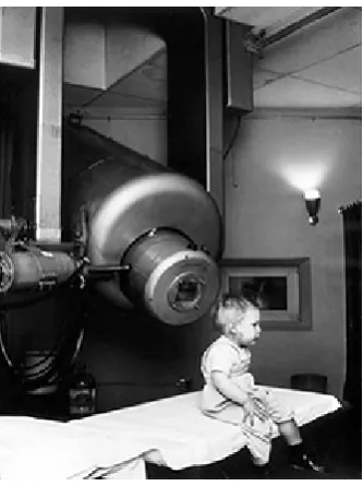
1.5 Baby Gordon Isaacs being treated for retinoblastoma 1957 . . . 5
1.6 The differences between conventional radiotherapy, conformal radio-therapy CFRT and CFRT with intensity modulation IMRT . . . 6
1.7 Differences between proton and photon therapy . . . 7
1.8 The Bragg Peak . . . 8
1.9 Possible effects of range uncertainties. . . 9
1.10 Prompt Gamma Imaging . . . 10
1.11 Positron Emission Tomography . . . 11
1.12 The PRaVDA pCT system concept . . . 12
1.13 The ProTom Radiance 330 proton therapy system . . . 13
1.14 he PSI 590 MeV high intensity 8-sector Ring Cyclotron (HIPA) . . 14
1.15 The NORMA NORMAl conducting racetrack medical FFAG . . . . 15
1.16 The IMPULSE cyclinac concept . . . 16
1.17 Artist’s Impression of The Christie Rutherford proton Centre. . . . 17
1.18 The Varian Probeam multi-room proton therapy system . . . 18
1.19 The Varian Probeam 253 MeV cyclotron being delivered at the Christie 19 1.20 Layout of the proton therapy facility at The Christie Hospital . . . 19
1.21 Compact gantry design and gantry room in the Christie . . . 20
2.1 Electric and magnetic fields for the transverse-magnetic resonant mode in a cylindrical cavity . . . 22
2.2 Beam bunches in the positive phase of an RF voltage . . . 23
16 List of figures
2.4 The transit time factor vs the ratio of the length of the gapg to the
distance a particle travels in one RF wavelength . . . 25 2.5 Graphical representation of the phase stability principle whereby
the synchronous phase can keep a particle stable in the bunch. . . . 27 2.6 Separatrix used in longitudinal beam dynamics . . . 28 2.7 Golf club separatrix . . . 29 2.8 A particle’s trajectory through a drift space of lengthLD the
defini-tions of x and x’ are shown . . . 30 2.9 The phase space ellipse in terms of Courant-Snyder or ‘Twiss’
pa-rameters . . . 31 2.10 Typical FODO arrangement with focussing quadrupoles (blue)
defo-cussing quadrupoles (green) and RF cavities (red) in the drift spaces between. . . 32 2.11 Typical FODO arrangement with focussing quadrupoles (blue)
defo-cussing quadrupoles (green) and drift spacesLD between. . . 33
2.12 Effective potential barrier seen by the conducting electrons in bulk metal . . . 36 2.13 The electric field distribution on a logarithmic scale around a
cylin-drical emitter . . . 36 2.14 Field enhancement factor for various possible emitter geometries . . 37 2.15 BDR dependence on accelerating gradient with both the defect model
fit and the power law fit . . . 39 2.16 BDR dependence on electric field fitted with theoretical lines based
on a stochastic model of breakdown nucleation . . . 39 2.17 Illustration of the different stages of Radio Frequency (RF) breakdown 41 2.18 The shape and temperature distribution of a nano-tip during intense
electron emission . . . 42 2.19 Time dependences of electric field, active power flow, reactive power
flow, and field emission power flow . . . 44 2.20 Square root of the scaled modified Poynting vector calculated for
the high-gradient performances of several structures . . . 45 2.21 Absolute part of the electric field inside a re-entrant pillbox cavity . 50 2.22 Equivalent circuit model of an RF cavity . . . 50 2.23 ‘electric’ or ‘capacitive’ coupling through the iris of a pillbox cavity 52 2.24 ‘magnetic’ or ‘inductive’ coupling through coupling slots in the end
cap of the pillbox cavity . . . 52 2.25 Equivalent circuit for one cell of a periodic array of electrically
List of figures 17
2.28 Dispersion for magnetically coupled resonators . . . 53
2.29 Power filling comparison between standing and travelling wave struc-tures . . . 55
2.30 Field profiles of the 0-mode, π-mode and π/2-mode adjusted from . 55 2.31 Modes in the passband of a resonant structure . . . 56
2.32 π/2 mode in a) A periodic structure b) A bi-periodic on-axis coupled-cavity structure and c) A bi-periodic side-coupled coupled-cavity . . . 57
2.33 Dispersion curve of a bi-periodic structure . . . 58
2.34 The relativistic β vs Kinetic Energy (MeV) . . . 59
2.35 Summary plot of CLIC high gradient structures. . . 59
2.36 An Alverez drift-tube linac . . . 60
2.37 An Widroe drift-tube linac . . . 60
2.38 H-Mode cavities . . . 61
2.39 Effective shunt impedance of low-β normal conducting structures . 62 2.40 PIMS cavity under test in CERN’s main workshop . . . 63
2.41 805 MHz SNS side-coupled cavity. Two segments are joined by a bridge coupler. . . 64
2.42 Annular coupled structure at J-PARC. . . 64
2.43 805 MHz SRF cavity at SNS. . . 65
2.44 704 MHz SRF cavity at ESS. . . 65
2.45 Various low, medium, and high-β SRF cavity designs. . . 66
2.46 LIBO structure RF measurement set up. . . 67
2.47 Complex magnitude electric field distribution inside the bTW cavity 67 2.48 Mechanical view of structures optimised by TERA forβ=0.38 . . . 68
2.49 Effective shunt impedance as a function ofβ for various low-β cavities. 69 2.50 The dispersion curve of a disk-loaded periodic waveguide structure with magnetic coupling . . . 70
3.1 A pillbox cavity vacuum model (left) Electric field profile (centre) and magnetic field profile (right). . . 73
3.2 The peak surface electric field (left) and peak surface magnetic field (right) both normalised to the accelerating gradient. . . 74
3.3 The shunt impedance per unit length and √Sc normalised to Eacc. . 75
3.4 The shunt impedance per unit length and the aperture radius divided by the wavelength of each respective frequency. . . 75
3.5 The absolute electric field peaking around the beam aperture for a 12 GHz pillbox cavity with a re-entrant section. . . 76
18 List of figures
3.7 The increase in gradient for a 2 mm radius aperture with the addition of a re-entrant. Gradient limited by 50 MW/m andSc=4 W/µm2. . 77
3.8 The maximum gradient calculated for a re-entrant pillbox cavity at a range of frequencies and aperture radii. The septum thickness is scaled with frequency the input power is 100 MW/m, and Sc is
limited to 4 W/µm2. Plot courtesy of Graeme Burt. . . 78
3.9 Diagram labelling the parameters on a nose cone geometry. . . 79 3.10 The effect of the gap between the nose cones on shunt impedance
and peak fields for both S and X-band. . . 80 3.11 The effect of the nose cone radii on shunt impedance and peak fields
for both S and X-band. Rx on the x-axis refers to the radii in the
plot legend. . . 81 3.12 The effect of the nose cone angle on shunt impedance and peak fields
for both S and X-band. . . 82 3.13 The effect of the flat section of the nose cone on shunt impedance
and peak fields for both S and X-band. . . 83 3.14 How the coupling requirement to maintain correct phase and field
flatness varies with structure length and frequency. . . 85 3.15 Peak surface magnetic field plot of the side-coupled CST model and
the coupling slot geometry. . . 86 3.16 Thek-factor can be increased by increasing the length of the coupling
slot while having less of an effect on the shunt impedance than increasing the slot depth. . . 87 3.17 Side-coupled vacuum model and the electric field of theπ/2-mode.
This structure had the maximum achieved k-factor at 17.6%. . . 87
3.18 Novel side-coupled cavity design where the inter-cell coupling is maximised . . . 88 3.19 12 GHz X-band side-coupled vacuum quadruplet (left) - electric field
Ez (right). . . 89
3.20 A 12 GHz X-band Side-Coupled Quadruplet. Modified Poynting Vector Sc peaking on the coupling slot. . . 90
3.21 Optimisation ofZ using the gap between the nose cones. . . 91
3.22 3 GHz S-band side-coupled quadruplet vacuum model (left). Electric field Ez (right). . . 92
3.23 3 GHz S-band Side-coupled quadruplet. Nose cone gap optimisation. Gradient is limited byScand shunt impedance with 50 MW/m input
power. . . 92 3.24 Shunt impedance and unloaded Q-factor reduction with increase in
List of figures 19
3.25 Modified Poynting vector peaks on the nose cone of the 3 GHz side-coupled SW structure as opposed to the coupling slot. . . 95 3.26 Maximum gradient achieved for side-coupled standing wave
struc-tures of different lengths and frequencies. Gradient is limited by 50 MW/m input power and available shunt impedance using
Sc≤4W/µm2 as a peak field limit. . . 96
3.27 Dispersion diagrams of increasing numbers of circular couplings slots. Only the 16 slot structure exhibits a Backwards Travelling Wave (bTW). . . 97 3.28 Electric field profiles of circular couplings slots. Various numbers of
coupling slots are shown. 4 Slots (left) 8 slots (centre) and 16 slots (right).Only the 16 slot structure exhibits a bTW. . . 97 3.29 Approximate optimum group velocity for a cell phase advanceφ of
2π/3. . . 98
3.30 Geometries of the coupling slots studied. . . 100 3.31 Definitions of ‘Angle’ and ‘Position’ in coupling slot optimisation. . 100 3.32 The effect of varying coupling slot parameters on the group velocity
of the wave in the structure for φ= 23π. . . 101
3.33 Shunt impedance data with group velocity shown on colour bar for
φ= 23π. . . 102
3.34 The similarity in geometry between 8 circular slots and 8 racetrack slots. . . 102 3.35 The peak surface magnetic field data with group velocity shown on
colour bar for φ= 23π. . . 103
3.36 The peak modified Poynting vector field data with group velocity shown on colour bar for φ= 23π. . . 104
3.37 Shunt impedance of structures with varying phase advances. ϕ in
this plot represents the slot angle ψ for the only structures with
fixed ψ. . . 104
3.38 Normalised peak electric field of structures with varying phase ad-vances. ϕ in this plot represents the slot angle ψ for the only
structures with fixed ψ. . . 105
3.39 Normalised peak magnetic field of structures with varying phase advances. ϕ in this plot represents the slot angle ψ for the only
structures with fixed ψ. . . 105
3.40 Normalised modified Poynting vector of structures with varying phase advances. ϕ in this plot represents the slot angle ψ for the
only structures with fixed ψ. . . 106
3.41 The electric field profile for a 12 GHz single cell cavity φ= 23π with
20 List of figures
3.42 The modified Poynting vector and gradient across a 60 cell 12 GHz
φ= 26π constant impedance structure. The red bar indicates the
max-imum allowable Sc and the blue bar indicates the overall structure
gradient of 55 MV/m. . . 108
3.43 The modified Poynting vector and gradient across the 60 cell 12 GHz
φ= 26π constant gradient structure. The red line indicates the peak Sc limit. . . 109
3.44 Sc of the first, middle, and last cell of the hybrid φ= 23π structure
from left to right. The group velocity is decreased through the structure by tapering the coupling slots. . . 109 3.45 The modified Poynting vector and gradient across the 60 cell 12 GHz
φ= 26π hybrid constant impedance/constant gradient structure. The
red line indicates the maximum allowable Sc and the blue line
indicates the overall gradient of the structure: 58.9 MV/m. . . 110
3.46 The modified Poynting Vector distribution for 12 GHz single cell cavity φ= 56π with 8 racetrack coupling slots. . . 110
3.47 The modified Poynting vector and gradient across the 48 cell 12 GHz
φ= 56π constant impedance structure.The red line indicates the
maximum allowableScand the blue line indicates the overall gradient
of the structure: 57.6 MV/m. . . 111
3.48 The modified Poynting vector and gradient across the 47 cell 12 GHz
φ= 56π constant gradient structure. . . 111
3.49 The modified Poynting vector and gradient across the 24 cell 12 GHz
φ= 56π constant impedance structure. Red line indicates the
maxi-mum allowable Sc whilst the blue line indicates the overall structure
gradient 59.1 MV/m. . . 112
3.50 The modified Poynting vector and gradient across the 24 cell 12 GHz
φ= 56π constant gradient structure. The red line indicates the peak Sc limit. Gradient = 65 MV/m. . . 113
3.51 CLIC superstructure installed at CTF3 . . . 113 3.52 The modified Poynting vector distribution of a 3 GHz φ= 23π bTW
structure with a vg/
c of 0.07%. . . 114
3.53 Single cell pillbox cavity with a re-entrant section with a 1.75 mm
aperture. Peak fields are limited by Sc alone and which results in
high peak surface electric fields. The gradient has been calculated with the available input power and shunt impedance. . . 115 3.54 Figure showing maximum gradient with and without re-entrant and
List of figures 21
4.1 Scaling fits taken from the TERA Foundation (TERA) publication
on the 3 GHz single cell high gradient test results . . . 120
4.2 Absolute component of the electric field profiles of S- and C-band travelling wave structures investigated at 4 mm aperture. Initially 16 coupling slots were implemented for the C-band (centre) structure but vg was limited by space between slots so 8 slots were used (right).121 4.3 Nose cone optimisation process for S-bandφ=56π single cell structure. The gradient is calculated with the available shunt impedance and 12.8 MW input power per structure. Legend indicates the nose cone angle. . . 123
4.4 C-band constant gradient backwards travelling wave structureφ=56π peak fields and gradient limited by 12.8 MW input power and avail-able shunt impedance. Red lines indicate maximum allowavail-able values for each respective plot. . . 125
4.5 S-band constant gradient backwards travelling wave structureφ=56π peak fields and gradient limited by 12.8 MW input power and avail-able shunt impedance. Red lines indicate maximum allowavail-able values for each respective plot. . . 126
4.6 Cross section of S-band side-coupled standing wave structure quadru-plet model used in simulation with periodic boundaries. Electric field plot showing the π 2 mode. . . 127
4.7 Magnetic field profile of a C-band side-coupled quadruplet. . . 128
4.8 The prototype Quadruplet electric field distribution. . . 132
4.9 Peak E-field (Z) in the final side-coupled quadruplet . . . 132
4.10 Power coupler added to the optimised quintuplet . . . 133
4.11 Z-component of the E-field inside the coupling cell with power coupler (not pictured) with two ordinary coupling cells. Unwanted fields are shown in the side-coupled cells . . . 134
4.12 Z-component of the E-field inside the coupling cell with power coupler (not pictured) with two ordinary coupling cells . . . 135
4.13 Electric field along the beam axis of the three cell power coupler model135 4.14 S-parameters and E-field along beam axis for 3-cell coupler model . 136 4.15 End cell model . . . 137
4.16 Z-component of E-field along the beam axis of the end cell model . 137 4.17 CST vacuum model of the 11-cell prototype structure . . . 138
4.18 Magnitude of the electric field along axis of the 11-cell prototype structure . . . 138
22 List of figures
4.21 Electric field distribution along the beam axis of the prototype model after final optimisation (Top). S-parameters of prototype structure after final optimisation simulations (Bottom). . . 140 4.22 Dispersion curve of the final prototype structure. The stop-band
between the two π/2 modes has not been adequately closed. . . 141
4.23 Ez of the accelerating mode of the final prototype structure at
2.99869 GHz. . . 142 4.24 The Z-component of the electric field on axis of the accelerating
mode of the final prototype structure. . . 142
5.1 Timing diagram for the cyclinac scheme, showing, from top to bottom, the linac RF pulses, the cyclotron pulses, the linac RF in each pulse and the proton intensity profile . . . 144 5.2 Typical beam envelope through an RF cavity . . . 146 5.3 The allowed phase space region through an RF cavity and the largest
phase space ellipse possible inside of it . . . 147 5.4 Linac layout as it was set up in ASTRA . . . 151 5.5 Maximum and minimum beta-functions as a function of the betatron
phase advance . . . 152 5.6 Results of the large aperture particle tracking study . . . 154 5.7 Maximum and minimum beta functions . . . 155 5.8 Transverse and longitudinal transmission, total transmission and
required gradient vs. number of cells per cavity . . . 157 5.9 Transmission through 7×3-cell cavities and matching sections between158
5.10 Transmission through 7×7-cell cavities and matching sections between159
5.11 Transmission through 6×11-cell cavities and matching sections between160
5.12 Transmission through 5×15-cell cavities and matching sections between161
6.1 The simulation model for the ‘push’ tuning studs and a plot showing the resulting frequency shift in Hz. The x-axis is how many mm the tuning stud has been inserted into the cavity wall. . . 164 6.2 The simulation model for the ‘pull’ tuning studs and a plot showing
the resulting frequency shift in Hz. The x-axis is how many mm the tuning stud has been pulled from the cavity wall. . . 164 6.3 Tuning studs in assembly with the ceramic pins used to hold studs
in position during brazing. . . 165 6.4 Slide-hammer used to push and pull the tuning studs . . . 165 6.5 Temperature distribution of the cavity at steady state with 4 kW
average power. . . 169 6.6 Maximum temperature difference across the cavity from 0.5-4 kW
List of figures 23
6.7 The absolute displacement field consequent of the 4 kW average RF heating the structure. Displacement is with respect to the fixed knife edge of the flange on the input coupler. . . 171 6.8 Maximum displacement from thermal expansion. Red dashed line is
a fit. . . 171 6.9 Simulated deformation of the cavity at steady state with an average
power of 4kW magnified by 1000×. . . 172
6.10 Displacement field map in the Z direction. Parameters ‘Septum’ and ‘Length’ are also shown. . . 172 6.11 Estimated operational detuning for a range of input powers.
Maxi-mum allowable shift shown at 230 kHz. . . 175 6.12 Cooling capacity of the chiller anticipated for testing . . . 176 6.13 Pump capacity of the chiller anticipated for testing . . . 177 6.14 Previous manufacturing techniques for side-coupled cavities . . . 179 6.15 One disk per cell cut. . . 179 6.16 Interlocking alignment technique. . . 180 6.17 Magnetic peak field on the coupling slot. . . 180 6.18 The difficult to access coupling slot. . . 181 6.19 Alternative cut with 2 disks per cell. . . 181 6.20 Precision surfaces were added to the disks for alignment. . . 182 6.21 Tooling to clamp the machined disks together to do an initial RF
measurement before bonding. (image courtesy of Lancaster University)182 6.22 Final rendered image of Proton Boosting Extension for Imaging and
Therapy (ProBE) cavity. Magnification of the alignment surface highlighted in red. . . 183 6.23 Disk after pre-machining stage of manufacture. . . 183 6.24 Figure shows the alignment, and weight tools for hydrogen bonding of
the disks. After the disks have been bonded together the remaining pieces are brazed on in various steps of decreasing temperature. (Design and images courtesy of Niklas Templeton at Daresbury
Laboratory, UK. . . 185 6.25 Temperature profile for bonding process under H2 partial pressure . 186
6.26 Disk after pre-machining stage of manufacture. . . 186
7.1 The S-band high gradient test bench installed in CTF2 at CERN as part of the CLIC high power test program. . . 187 7.2 Conditioning history of a TD26CC prototype tested at X-box 1
(CERN) . . . 189 7.3 Functional diagram of the S-box experiment at CERN. . . 190 7.4 The high power set up of the S-box experiment. Featuring modulator
24 List of figures
7.5 The S-box electronics rack in the CTF3 klystron gallery. . . 192 7.7 Fourier transform of frequencies out of the original down-mixer. . . 194 7.8 The revised down-mixer schematic . . . 195 7.9 A normal pulse including incident power, reflected power,
transmit-ted power and Faraday cup signals. . . 196 7.10 Simulated total structure reflection as a function of the breakdown
positioning along the structure . . . 197 7.11 A breakdown pulse detected by the Faraday cup signals. The red and
blue traces below zero are the Faraday cups signals. The incident (green), reflected (pink) and transmitted (red) signals are above zero.198 7.12 A breakdown pulse detected by the reflected signal. The red and
blue traces below zero are the Faraday cups signals. The incident (green), reflected (pink) and transmitted (red) signals are above zero.199 7.13 S-box operational screenshot. . . 200 7.14 Screenshot of the ‘RF Control’ VI including the conditioning
algo-rithm (top left). . . 200 7.15 The conditioning history of the KT structure . . . 202 7.16 BDR with respect to the accumulated number of pulses during
conditioning at constant power . . . 203 7.6 The original down-mixer design for the S-box experiment . . . 205
8.1 Final machined disks after delivery by VDL. . . 208 8.2 One of the final disks provided by VDL. This particular cell was
List of tables
2.1 Frequency scaling laws . . . 49
3.1 The nominal nose cone parameters used in the nose cone optimisation study. . . 79 3.2 Summarises the effect of nose cones and coupling on the effective
shunt impedance of a 12 GHz pillbox cavity. . . 89 3.3 Nose cone parameters for a 12 GHz side-coupled structure . . . 90 3.4 The parameters for the 12 GHz side-coupled standing wave cavity.
Gradient limited by 12.8 MW input power. . . 90
3.5 The parameters for the 3 GHz side-coupled standing wave cavity. Gradient is limited by 12.8 MW input power. . . 93
3.6 Approximate Q-factor values for the selection of frequencies consid-ered in this study. . . 99
4.1 Minimum nose cone parameters considered in the large aperture optimisation. . . 122 4.2 Parameters for single cell φ=5π/6 backwards travelling wave
struc-tures. Gradient is limited by 12.8 MW input power with available shunt impedance. Both are limited by peak surface electric field. . . 124 4.3 Parameter table for the 5.7 GHz side-coupled standing wave cavity.
Gradient is limited by 12.8 MW input power, and available shunt
impedance. . . 127 4.4 Parameter table for the 3 GHz side-coupled standing wave quadruplet.
Gradient is limited by 12.8 MW input power, and available shunt
impedance. . . 129 4.5 parameters for each large aperture structure considered with the
26 List of tables
4.6 Parameters for the final prototype structure - Gradient limited by 12.8 MW input power and available shunt impedance. . . 131
5.1 Generic cyclotron parameters used to create the initial particle distribution in the cavity length study. . . 153 5.2 Summary of the final linac design parameter after the cavity length
study. . . 162
6.1 Table containing the tolerance sensitivity of the ProBE prototype cavity. . . 167 6.2 Estimated frequency shift due to 3 kW average input power. df/dz
are the frequency shifts calculated in Table 6.1 for 1µm shift and
the second set of frequency values are from 10µm deformation. Disp.
is the displacement in µm taken from CST field maps as shown in
Figure 6.7. . . 174
7.1 Comparison between the main design parameters of the KT bTW structure and ProBE. . . 204
8.1 The parameters for the final prototype structure. Gradient is limited by 12.8 MW input power and available shunt impedance. . . 211
8.2 Summary of the final linac optics design parameters. . . 212
Glossary
ε0 Permittivity of free space.
σc Electrical conductivity.
βF E Field enhancement factor.
βs Relativistic velocity of the synchronous particle.
βT Twiss β - betatron amplitude function.
ϕW F Work function.
A Atomic mass.
ACS Annular Coupled Structure.
ADAM An advanced oncotherapy company.
ADC Analogue to Digital Converter.
ASTRA A Space Charge Tracking Algorithm.
AVF Azimuthally Varying Field.
AVO Advanced oncotherapy.
B Magnetic field.
Bpeak Peak surface magnetic field.
BDR Breakdown rate.
β Relativistic velocity.
bTW Backwards Travelling Wave.
C Minimum circumference of RF cavity.
28 Glossary
cϵ Specific heat capacity.
Cp Specific heat capacity at constant pressure.
CCC CERN Control Centre. CCL Coupled Cavity Linac.
CERN Organisation européenne pour la recherche nucléaire.
CFRT ConFormal Radio-Therapy. CLIC Compact LInear Collider.
CMOS Complimentary metal-oxide-semiconductor.
CST Computer simulation technology.
CT Computed tomography. CW Continuous Wave.
d Coupling slot depth.
δ Skin depth.
DTL Drift-Tube Linac. DUT Device Under Test.
E Electric field.
E0 Axial electric field. Eacc Accelerating gradient.
EF Fermi Level.
Ek Kilpatrick limit.
Epeak Peak surface electric field.
Er Rest energy.
Es Energy of the synchronous particle.
ε Geometric emittance.
ES Energy selection.
Glossary 29
η Dynamic viscosity.
F Force.
f Frequency.
fD Darcy friction factor.
FFAG Fixed Field Alternating Gradient.
∆H full width half maximum.
g Accelerating gap.
Gc Gap between the nose cones.
Γ Reflection coefficient.
γs Lorentz factor of the synchronous particle.
GUI Graphical User Interface.
h Heat transfer coefficient.
Hϕ Hamiltonian of the system.
HG High Gradient.
HIPA High Intensity 8-sector Ring Cyclotron.
HU Hounsfield Units.
IF N Field emission current.
IARC International Agency for Research on Cancer’s.
IDRA Institute for Diagnostics and RAdiotherapy.
IF Intermediate Frequency.
IFIC Institut de Física Corpuscular.
IMPULSE IMaging and Intensity Modulation PULSEd energy booster.
IMRT Intensity-Modulated Radio-Therapy.
INFN Istituto Nazionale di Fisica Nucleare.
30 Glossary
K K-strength of a quadrupole. k Coupling factor.
kB Boltzmann’s constant.
κ Thermal Conductivity.
KT Knowledge Transfer.
l Cavity cell length. Lcav Cavity length.
LD Drift Length.
lq Length of a quadrupole.
lsc Coupling cell length.
λ Wavelength.
LHC Large Hadron Collider.
LIBO LInear BOoster.
LIGHT Linac for Image Guided Hadron Therapy.
linac Linear accelerator. LLRF Low Level RF. LPM Litres per minute.
˙
m Mass flow rate.
me Mass of an electron.
MAD-X Methodical Accelerator Design. MRI Magnetic Resonance Imaging.
NA Avogadro’s number.
Nbd Number of breakdowns.
Ncell Number of accelerating cells.
Np Number of RF pulses.
Glossary 31
NMR Nuclear Magnetic Resonance.
NORMA NOrmal-conducting Racetrack Medical Accelerator. Nu Nusselt number.
OAR Organ at risk.
ω angular frequency.
Pd Power dissipated per cycle.
Pin Input power.
PT Travelling wave power.
PAMELA Particle Accelerator for MEdicaL Applications. pCT proton Computed Tomography.
PEC Perfect electric conductor. PET Positron Emission Tomography.
φ Phase advance.
PID Proportional Integral Derivative.
PIMS PI-Mode Structure. PLL Phase Locked Loop.
PMQ Permanent Magnet Quadrupole.
Pr Prandtl number.
PRaVDA Proton Radiotherapy Verification and Dosimetry Applications.
ProBE Proton Boosting Extension for Imaging and Therapy. PSI Paul Scherrer Institute.
PSP Proton Stopping Power.
˙
Q Heat transfer rate. q Charge of a particle.
32 Glossary
Ql Loaded quality factor.
rap Aperture radius.
rc Cavity radius.
re Classical electron radius.
Rin Inner nose cone radius.
Ron Outer nose cone radius.
Rs Effective shunt impedance.
rsc Coupling cavity radius.
Rsurf Surface resistance.
Re Reynold’s number.
RF Radio Frequency.
RFQ Radio-Frequency Quadrupole.
ρr Resistivity.
rms Root mean squared.
RSS Root sum squared.
S Septum thickness.
SC Modififed Poynting Vector.
Sc Modified Poynting Vector.
SCS Side Coupled Structure.
SCSWS Side-coupled standing wave structure. SNS Spallation Neutron Source.
SRF Superconducting Radio-Frequency. SRT Stereotactic Radio-Therapy.
SµS Swiss Muon Source.
SWS Standing-Wave Structure.
Glossary 33
tf ill filling time.
tp Pulse length.
TE Transverse Electric.
TEM Transverse Electro Magnetic.
TERA Fondazione per Adroterapia Oncologica.
TM Transverse Magnetic.
TOP-IMPLART Terapia Oncologica con Protoni - Intensity Modulated Proton Linear Accelerator for Radiotherapy.
TULIP TUrning LInac for Proton therapy.
TWS Travelling-Wave Structure.
U Stored energy.
Ud Energy dissipated per cycle.
UHV Ultra-High Vacuum.
v velocity.
Vϕ Potential energy.
V0 Voltage across a cavity.
Vc Acceleration voltage (V0T).
vg Group velocity.
vp phase velocity.
VCO Voltage Controlled Oscillator.
VI Virtual Instrument.
Chapter 1
Proton Therapy, Imaging &
Accelerators
Cancer has been and will continue to be one of the greatest healthcare challenges of the 21st century. Over 18 million new cancer cases were diagnosed in 2018,
alongside 9.6 million cancer deaths, and 43.8 million people reported to be living with cancer according to the International Agency for Research on Cancer’s (IARC) GLOBOCAN database. This is predicted to rise to 24.1 million new cancer cases in 2030, with over 13 million cancer deaths [1]. The estimated cancer incidences and deaths from 2018 up to 2040 are shown in figures 1.1 & 1.2. Advancing development of diagnostic methods, such as computer-aided imaging and increased precision in radiation therapy, has seen the cure rates of cancers diagnosed pre-metastasis steadily improve over recent decades [2]. Further improvement of cure rates will be a result of further development of these techniques and also from the rapid transfer of these improved methods into clinical practice. The application of physics to medicine is not a new phenomenon, the first ever Nobel prize in physics was awarded to Wilhelm Conrad Röntgen in 1901 for discovering the X-ray. Figure 1.3 shows the famous image he created of his wife Anna Bertha Ludwig’s hand.
Linear accelerators (linacs) have been used in medicine since the 1950s [3], and in 2005 7500 linear electron accelerators were being used for radiotherapy worldwide [4]. Photon radiotherapy was first used to treat cancer and has long been the predominant treatment, but in 1947 Robert Wilson suggested it may be beneficial to use heavy charged particles instead [5]. Proton therapy better spares organs at risk (OARs) from a radiation dose than photon radiotherapy. Sparing OARs also requires accurate imaging techniques. Imaging with protons (pCT) during treatment planning is foreseen to improve the ballistic selectivity of proton beam radiotherapy [6–8], even further beyond that ofphoton radiotherapy
2 Proton Therapy, Imaging & Accelerators
Fig. 1.1 Estimated number of incident cancer cases from 2018 to 2040, all cancers, both sexes, all ages [1].
Fig. 1.2 Estimated number of cancer deaths from 2018 to 2040, all cancers, both sexes, all ages [1].
In this work we explore the feasibility of upgrading existing proton therapy centres fitted with 250 MeV cyclotrons with a linear accelerator to provide 350 MeV protons. This is foreseen to improve the accuracy of proton therapy treatments by providing proton imaging, and be far reaching in its accessibility to most existing proton therapy centres.
1.1
Medical Proton Accelerators
1.1 Medical Proton Accelerators 3
Fig. 1.3 Hand mit Ringen (Hand with Rings): a print of one of the first X-rays by Wilhelm Röntgen (1845–1923) of the left hand of his wife Anna Bertha Ludwig. It was presented to Professor Ludwig Zehnder of the Physik Institut, University of Freiburg, on 1 January 1896 [9].
The next advance in medical accelerators was the betatron [14], capable of producing electron beams from 5 to 25 MeV for use in radiotherapy. The betatron’s output energy was limited by the strength of the magnetic field possible due to the saturation of iron, and also due to the size of the magnet core. Figure 1.4 shows Kerst working on the first betatron where the magnet weighed 4-tons. Ultimately the betatron was no match for the invention that revolutionised radiotherapy to this day; the linear accelerator or ‘linac’.
The linac was first proposed by Widerøe in 1928 [16], so called because the path of the accelerated beam was linear. The small accelerating gradients (<10 MeV/m)
[image:37.595.233.401.68.312.2]4 Proton Therapy, Imaging & Accelerators
Fig. 1.4 Early betatron at University of Illinois. Kerst is at right, examining the vacuum chamber between the poles of the 4-ton magnet [15].
In recent years, greater understanding of RF cavities has lead to larger accel-erating gradients being achieved, which has reduced the size of linacs and made them more useful in medicine. A collaboration between TERA (Fondazione per Adroterapia Oncologica), European Organization for Nuclear Research (CERN), the university and Istituto Nazionale di Fisica Nucleare (INFN) of Milan and the university and INFN of Naples designed a high frequency proton linac for medical applications at 3 GHz. The LInear BOoster (LIBO) structure was designed to reach a gradient of 15.8 MV/m, but after a short conditioning time was able
to reach 28.5 MV/m[18]. It has been featured in both the Terapia Oncologica
con Protoni - Intensity Modulated Proton Linear Accelerator for Radiotherapy (TOP-IMPLART) project [19], and the Institute for Diagnostics and RAdiotherapy (IDRA) project [20]. The TOP-IMPLART linac is a 150 MeV pulsed proton linear accelerator for proton therapy applications under commissioning at ENEA Frascati. The IDRA (Institute for Diagnostic and RAdiotherapy) is a cyclinac with a 30 MeV commercial cyclotron followed by the LIBO structure accelerating to 210 MeV.
The cyclinac idea was first proposed by U. Amaldi in 1993 [21], where a booster linac is placed at the output of a cyclotron to reach higher energies. This concept is advantageous to hospitals due the simplicity and relative compactness of the cyclotron. Unfortunately the extraction frequency of most cyclotrons is in the MHz range, much lower than the high frequency linac sections which are GHz, and this mismatch is responsible for large beam losses at the start of the linac. Luckily low average currents in the nA range are required for radiotherapy and cyclotrons typically provide µA. Even less current is required for radiography; a few pA are
[image:38.595.196.361.70.273.2]1.2 Proton Therapy 5
Fig. 1.5 Baby Gordon Isaacs was the first patient to be treated with a linear accelerator at just 2 years old in 1957. His retinoblastoma was cured and he survived into adulthood with normal vision [17].
More recently the TERA foundation with the CERN Compact LInear Collider (CLIC) group designed and built a high gradient medical accelerating cavity for use in the TUrning LInac for Proton therapy (TULIP) all-linac project [22] funded
by the Knowledge Transfer (KT) group. With a nominal gradient of 50 MV/m, it
is the highest gradient proton accelerator demonstrated at this energy level.
1.2
Proton Therapy
[image:39.595.233.400.68.291.2]6 Proton Therapy, Imaging & Accelerators
and IMRT where the field is geometrically shaped similar to CFRT but is also intensity modulated pixel by pixel within the shaped field to account for varying tumour depths. Figure 1.7 illustrates the difference between SRT with traditional photon beams (left) and proton therapy (right). SRT approaches the tumour from all available angles around the patient. This results in a lower dose to the healthy tissue and a larger layered dose to the target volume. The region marked in green is the brain stem, and it is desirable to limit the dose to this region as much as possible. Proton beams offer an elegant solution, due to the way that they deposit energy exit dose can be minimised. Thus the proton therapy treatment (right) has no exit dose and has reduced the dose deposited in the brain stem in comparison to SRT.
Fig. 1.6 The differences between conventional radiotherapy (top), conformal radio-therapy CFRT (centre) and CFRT with intensity modulation IMRT (bottom) [23].
In 1947 Robert Wilson suggested that with high energy protons, precision irradiation of tumours was possible due to the unique dose deposition of moderately relativistic heavy charged particles [5], described by the Bethe-Bloch equation [28– 30]
−
*
dE dx
+
=kq2Z A
1
β2
"
1 2ln
2mec2β2γ2Tmax
I2 −β
2− δ(βγ)
2
#
[image:40.595.176.379.271.596.2]1.2 Proton Therapy 7
Fig. 1.7 Illustrates the differences between photon radiotherapy (left) where dose is deposited across the entire cross section of the patient and proton therapy (right) where the dose ends half way through, the back of the head, spine and back see no dose [27].
where −DdE dx
E
is the stopping power of the material or the energy loss (dE)
occurring over distancex. k= 4πNAre2mec2,NAbeing Avogadro’s number,rebeing
the classical electron radius,me being the mass of an electron andcbeing the speed
of light. q is the charge of the incident particle, Z and A are the atomic number
and atomic mass of the absorber respectively,I ≈11.5Z eV is the mean ionisation
potential, Tmax = 2mec2β2γ2/[1 + 2γme/M + (me/M)2] is the maximum kinetic
energy that may be imparted to a free electron in a single collision and introduces a minor dependence on the incident particle mass M. γ is the Lorentz factor and β is the relativistic velocity of the particle. δ(βγ) is a density correction term [31].
Equation 1.1 highlights that the depth at which the Bragg peak occurs depends on the initial energy of the proton beam. Figure 1.8 illustrates the variation in dose deposition with tissue depth. Whereas a traditional photon beam will result in both an entrance and exit dose, a proton beam deposits ≈50% of the energy
before the Bragg peak, ≈ 50% in the tumour leaving little to no exit dose [32].
[image:41.595.211.421.69.285.2]8 Proton Therapy, Imaging & Accelerators
Fig. 1.8 Protons deposit energy in water via the Bragg Peak. Multiple Bragg peaks can be utilised with varying energies, resulting in a cumulative flat top dose called the Spread Out Bragg Peak (SOBP) [33].
1.2.1
The Range Problem
Due to the steep dose fall off distal to the Bragg peak, proton therapy has the potential to deliver higher doses to cancerous tissue while greatly reducing the dose delivered to healthy tissue in comparison to photon radiotherapy this is illustrated in Figure 1.9(a). This steep dose gradient distal to the Bragg peak is not used to spare OARs in practice because of uncertainties around its exact location in the patient. Figure 1.9(b) illustrates the influence of uncertainties on different depth-dose curves. In the case of traditional photon radiotherapy a small uncertainty in the dose delivery makes a small difference to the dose seen by both the tumour and the organ at risk (OAR), in all three curves the peak occurs in the soft tissue. In the case of proton radiotherapy, the same uncertainty can be the difference between the peak dose being deposited entirely in the tumour or entirely in the organ at risk. To benefit from the advantage of the Bragg peak clinicians must know with certainty where it will be deposited.
1.2 Proton Therapy 9
Fig. 1.9 (a) Potential dose benefit of a proton treatment compared to a photon treatment (dotted line: photon depth-dose curve; dashed line: mono-energetic proton depth dose curve known as Bragg Peak; straight line: spread out proton Bragg curve (SOBP) to cover the whole tumour). (b) Influence of uncertainties to these depth-dose curves [34].
10 Proton Therapy, Imaging & Accelerators
shown that this seemingly small inaccuracy results in PSP prediction errors of over 2% [44], and this is widely believed to be a main factor preventing proton therapy reaching its full potential.
1.2.2
Range Verification
in vivo
There are multiple approaches to managing range uncertainty in proton therapy [45– 48], but it will always be deemed necessary to verify proton rangein vivo be it by
directly measuring dose or fluence, or by indirectly measuring secondary emission caused by proton irradiation.
Prompt Gamma Imaging
On their path through the patient, protons undergo nuclear reactions with tissue and some of these interactions produce prompt gammas. After an interaction with a proton, the target nucleus is excited to a higher energy state causing a single photon known as a ‘prompt gamma’ to be emitted, returning the nucleus to its ground state (see Figure 1.10). The emitted gamma rays can then be detected.
As the protons traverse the patient they lose energy and their reaction cross sections decrease. This means proton interactions occur along the whole penetration path until 2-3 mm before the Bragg peak. Thus the emission of prompt gammas is related to the penetration path of the protons and conclusions can be drawn on the proton range.
The emission of prompt gammas happens during proton therapy whether or not they are being detected. One of the main advantages of this method is real-time verification of dose delivery, and no additional dose is imparted onto the patient. However, this also means prompt gamma imaging can not aid treatment planning efforts. Research into a suitable detector system is ongoing, but so far position verification of the Bragg peak of a 100 MeV proton beam in a phantom has been reported with 1-2 mm accuracy [49].
1.2 Proton Therapy 11
Positron Emission Tomography
In the previous example we discussed one outcome of protons’ interaction with nuclei - prompt gammas. Another interaction that can occur is the emission of a positron which then annihilates with an electron in surrounding tissue. Coincident gammas are subsequently emitted (see Figure 1.11) and can then be detected with a gamma camera. This is called Positron Emission Tomography (PET).
Similarly to prompt gamma imaging, PET has the advantage of not resulting in any additional radiation dose to the patient. PET imaging can either happen in real time or a certain time after the treatment is completed. It cannot however be used for treatment planning prior to the first treatment.
Fig. 1.11 Figure illustrates the concept behind positron emission tomography (PET) protons interact with nuclei in tissue and emitted positrons annihilate with electrons which then emits coincident gammas [51].
Magnetic Resonance Imaging
Nuclear Magnetic Resonance (NMR) Imaging or MRI is commonly used in hospitals to image soft tissue. A strong magnetic field is applied to the patient which excites the protons inside of the body. The excited protons emit an RF signal which is detected using a receiving coil. The rate at which excited protons return to their equilibrium state indicates which type of tissue those protons comprise.
Radiation can cause changes in the constitution of human tissue which can be visible by MRI. This method offers a high spatial resolution and doesn’t depart any additional radiation dose. Additionally, MRI scanners already exist in most hospitals and can be used for this type of range verification. Unfortunately it takes days [52] for the cells to actually change enough to be visible, in some cases only after the end of treatment. So although it can verify the range in vivo, it can not be used to directly measure PSP or to adapt therapy during the course of treatment to compensate for observed range errors [52].
Proton Computed Tomography
[image:45.595.235.398.264.352.2]12 Proton Therapy, Imaging & Accelerators
Radiotherapy Verification and Dosimetry Applications (PRaVDA) consortium [54]. Higher energy protons are used for pCT than the 250 MeV used for therapy. At least 330 MeV protons are needed to ensure that when they are sent through the patient and into the detector the Bragg peak occurs in a range telescope behind the patient instead of in the patient. One negative of proton imaging is that the patient will receive a small dose prior to treatment. However, images obtained using protons result in 50-100 times lower image exposure than x-ray radiographs of equal resolution [55].
In pCT a high energy proton beam is sent through two semiconductor detectors which record the x and y positions and direction on entry. After the patient the protons will exit through two more semiconductor detectors again recording the x and y positions and direction on exit. The protons are then bought to a stop in 24 layers of Complimentary metal-oxide-semiconductor (CMOS) sensors separated by absorbers, also referred to as a range telescope, which measures the exit energy. This process is repeated millions of times to collect lots of data, and the paths of the protons are reconstructed in software. The energy lost in the path the protons traversed in the body is thus calculated.
[image:46.595.93.481.379.643.2]1.3 Producing 350 MeV Protons 13
Despite the advantages of proton radiography it has not been adopted since its conception in 1960s[56] because of source availability and cost. To image full sized adult bodies 330-350 MeV [36] protons are required and this is where the high cost is incurred. There are efforts to provide proton therapy facilities with high energy protons and they are detailed in the next section.
1.3
Producing 350 MeV Protons
In recent years there have been multiple efforts to produce 330 MeV protons for a clinical setting. Figure 1.13 shows the ProTom Radiance 330 proton therapy system. The 330 MeV synchrotron allows for imaging and treatment with the same accelerator [57]. Injection beam line development is still ongoing to achieve the maximum dose rate of 2 Gy per minute per litre, and simulation and existing dose delivery tests suggest it will achieve that [58]. One benefit of this system is its variable extraction meaning no degrader is necessary resulting in a higher quality beam. However it has a large space requirement which some existing centres do not have.
Fig. 1.13 The ProTom Radiance 330 proton therapy system [57].
[image:47.595.109.526.390.670.2]14 Proton Therapy, Imaging & Accelerators
must vary either the magnetic field or the frequency. Synchrocyclotrons vary the RF frequency to accommodate the higher energy particles. These tend to have better focussing and can be made compact with high fields. However, one cannot have two separate bunches at different energies in the cyclotron at the same time, as one would not be synchronous. This limits the current that they can provide for a clinical setting. Isochronous cyclotrons vary the field with radius, but at higher energies this makes the beam hard to focus. Azimuthally Varying Field (AVF) cyclotrons vary the field with pole pieces and incorporate edge focussing which is limited at higher energies. At higher energies it is better to use many separate magnets or ‘sectors’, but this prevents the source injecting into the centre
of the cyclotron. The Paul Scherrer Institute (PSI) has constructed a 590 MeV High Intensity 8-sector Ring Cyclotron (HIPA) shown in Figure 1.14 which outputs 2.2 mA to feed the Swiss Muon Source (SµS) [59]. It has had issues with RF power
leakage into vacuum space [60], but 590 MeV protons are excessive for proton CT and this complication would likely cease with a lower energy output and custom flat top cavity. This was not designed for a medical application and is not an ‘all enclosed’ solution. The proton beam is pre-accelerated in a Cockcroft-Walton electrostatic column to an energy of 870 keV and this is increased to 72 MeV in the 4-sector Injector 2 cyclotron. Only then is the beam injected into the 8-sector 590 MeV cyclotron. This set up is much too big and complex for a hospital.
Fig. 1.14 The PSI 590 MeV high intensity 8-sector Ring Cyclotron (HIPA) [59].
1.4 The Project: ProBE: Proton Boosting Extension for Imaging and Therapy15
Racetrack Medical Accelerator (NORMA) (Figure 1.15) [64–66]. They are capable of producing 330 MeV protons rapidly with variable energy, but they have a large footprint and they are yet to be demonstrated.
Fig. 1.15 The NORMA NORMAl conducting racetrack medical FFAG [66].
A collaboration between PSI and the TERA proposed the IMaging and Intensity Modulation PULSEd energy booster (IMPULSE) [67] shown in Figure 1.16. This proposes the cyclinac concept to boost protons up to 350 MeV in a linac after a 250 MeV cyclotron used as a source for treatment. The linac proposes four 10 MW power sources to power 7 m of linac with an average gradient of 25 MV/m. More
technical information on the RF cavities in these various low-Relativistic velocity (β) systems can be found in Chapter 2.
1.4
The Project: ProBE: Proton Boosting
Ex-tension for Imaging and Therapy
[image:49.595.206.424.155.369.2]16 1. The Project: ProBE
Fig. 1.16 The IMPULSE cyclinac concept proposed by PSI and TERA [67].
treating patients this year. The protons used for treatment will be accelerated in the cyclotron to 253 MeV and transported to one of three treatment gantries shown in Figures 1.18 & 1.20. A fourth treatment room may be constructed but will remain empty initially to allow for a research/medical isotope room.
The ProBE project aims to examine the feasibility of upgrading the Christie proton therapy facility with a proton boosting linac, to accelerate the 250 MeV protons to 350 MeV, the energy required for pCT. Having the capability to image with protons in the same facility as treatment is one solution to the range problem detailed in section 1.2.1, and is expected to reduce patient treatment margins and improve patient outcomes. pCT systems are still in the development phase with research groups working on detector technology[71], image reconstruction[53], and producing a 350 MeV proton beam suitable for pCT. The Christie charity[72] has funded a research space utilising the real treatment beam from the Varian Probeam cyclotron. It is hoped this will facilitate the testing of the ProBE linac with a clinical beam, alongside other experiments such as radio-pharmaceuticals and pCT research which is already funded.
1.4.1
Three Stages:
Linac Development
[image:50.595.72.487.74.281.2]1. The Project: ProBE 17
Fig. 1.17 Artist’s Impression of The Christie Rutherford proton Centre [68].
fabrication was heavily influenced by the results obtained from the CLIC high gradient test programme [? ] at CERN to ensure the most reliable high gradient
operation. A beam dynamics study is also presented determining the best solution for adequate transmission through the linac. When fabrication of the cavity is complete it is foreseen to be conditioned and tested in the CLIC S-band high gradient test facility at CERN known as S-Box.
Linac Testing
Once the cavity testing is complete, the linac testing stage of the project can commence. As is shown in Figure 1.20 the fourth gantry room will be constructed at the same time as the rest of the facility, but patient treatment equipment will not be installed. Instead this room will become a research beam line with a length of around 10 metres. Here it will be possible to test the ProBE cavity with the real clinical beam. There will also be the capability at the Christie to test pCT detectors and conduct radio-biology amongst other research.
Superconducting Gantry
The third stage of the project is concerning beam delivery. Beam rigidity is defined as R= Bρ= p/q where B is the magnetic field, ρis the gyroradius of the particle
due to this field, p is the particle momentum, and q is it’s charge. At the high
energies necessary for proton imaging, beam rigidity is increased from 2.43 Tm at
250 MeV to 2.84 Tm at 350 MeV. Stronger magnets are necessary to manipulate
[image:51.595.107.526.70.280.2]18 1. The Project: ProBE
Fig. 1.18 The Varian Probeam multi-room proton therapy system. The fourth treatment room (right) at the Christie will have a superconducting gantry if they upgrade to higher energy protons [69].
1. The Project: ProBE 19
Fig. 1.19 The Varian Probeam 253 MeV cyclotron being delivered at the Christie [70].
[image:53.595.149.491.364.626.2]20 1. The Project: ProBE
Fig. 1.21 Top:Preliminary layout of the compact pCT gantry design; dipoles shown (curved) in black, quadrupoles shown in red. Bottom: visualisation inside the
[image:54.595.104.455.171.604.2]Chapter 2
RF Particle Acceleration
In this chapter, the theory of RF particle acceleration is introduced. The theory of RF cavities and the interaction of charged particles is presented, alongside important figures of merit to consider when designing RF cavities. Various RF cavity structures, specifically the current landscape of low/medium-β structures,
are described alongside RF breakdown phenomenology and other high gradient (HG) limitations. The Lorentz force law
F=q(E+v×B) (2.1)
is the most important equation in accelerator physics. It shows that electromagnetic fields can be used to accelerate and manipulate charged particles. It describes the force (F) of an electromagnetic field on charged particleq [75]. In the presence of an
electric field (E), a charged particleq will be accelerated in the direction of motion
of that electric field, therefore gaining energy. The force F is perpendicular to
both the magnetic field (B) and the particle velocity (v). Hence, the magnetic field
component does not increase the energy of the particle but adds a component of motion transverse to the initial direction of motion, bending the particle’s trajectory. It is because of this we can use electromagnetic fields to manipulate and accelerate charged particle beams for their desired use.
2.1
RF Cavities
A particle accelerator is made up of one or more RF cavities. An RF cavity is a hollow metallic structure that can be filled with electromagnetic fields, by an external high-frequency power source. The fields that exist inside a cylindrical cavity are given by
∇2− 1
c δ2 δt
!
E B
22 2. RF Particle Acceleration
Transverse Electro Magnetic (TEM) waves are not possible inside an RF pillbox cavity because to satisfy the boundary conditions either the electric or the magnetic field components must be in the direction of propagation. Assuming the cavity wall is a perfect electric conductor, the boundary condition is
Ez|Rcav = 0
for a Transverse Magnetic (TM) mode, and the magnetic field component is zero in the direction of propagation
Bz = 0.
For a Transverse Electric (TE) mode, the boundary condition is
δBz
δn
R
cav = 0
where δ/δn is normal to a point on the surface and the electric field component is
zero in the direction of propagation [76]
Ez = 0.
Fig. 2.1 Electric (E) and magnetic (B) fields for the transverse-magnetic resonant
TM010 mode in a cylindrical cavity [77].
Figure 2.1 shows the transverse-magnetic resonant mode (TM010) inside of a
cylindrical ‘pillbox’ cavity. The subscripts in TMmnp and TEmnp indicate different
mode patterns. In a rectangular cavity, m and n indicate the number of horizontal
periods and vertical periods respectively, and p is the number of longitudinal
periods in the direction of propagation. In a cylindrical cavity, m is the number
of full period variations of that field component in θ. n is the number of zeros of
[image:56.595.134.422.364.591.2]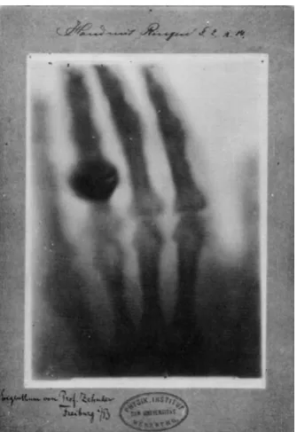
![Fig . 1 .4E a r lybe t a t r o n a t Univ e r s it yo f I llino is . K e r s t is a t r ig ht , e x a miningt hev a c uum c ha mbe r be t w e e n t he po le s o f t he 4 - t o n ma g ne t [1 5 ].](https://thumb-us.123doks.com/thumbv2/123dok_us/9304578.432012/38.595.196.361.70.273/fig-lybe-univ-llino-miningt-hev-uum-mbe.webp)
![Fig . 1 .6T he diff e r e nc e s be t w e e n c o nv e nt io na l r a dio t he r a pyt he r a py( t o p) , c o nf o r ma l r a dio -C FR T( c e nt r e ) a nd C FR Tw it h int e ns it ymo dula t io n I MR T( bo t t o m) [2 3 ].](https://thumb-us.123doks.com/thumbv2/123dok_us/9304578.432012/40.595.176.379.271.596/fig-diff-dio-dio-fr-fr-int-dula.webp)
![Fig . 1 .7I llus t r a t e s t he diff e r e nc e s be t w e e n pho t o n r a dio t he r a pyw he r e t he do s e e nds ha lf w a yde po s it e d a c r o s s t he e nt ir e c r o s s s e c t io n o f t he pa t ie nt a nd pr o t o n t he r a py( le f t ) w he r e do s e is( r ig ht )t hr o ug h, t he ba c ko f t he he a d, s pine a nd ba c ks e e nodo s e [2 7 ].](https://thumb-us.123doks.com/thumbv2/123dok_us/9304578.432012/41.595.211.421.69.285/fig-llus-diff-pho-pyw-nds-pine-nodo.webp)


![Fig . 1 .1 3T he P r o T o m R a dia nc e 3 3 0pr o t o n t he r a pys y s t e m [5 7 ].](https://thumb-us.123doks.com/thumbv2/123dok_us/9304578.432012/47.595.109.526.390.670/fig-t-r-dia-nc-pr-he-pys.webp)

![Fig . 1 .1 6T he I MP UL SEc y c lina c c o nc e pt pr o po s e d byP SI a nd T E R A [6 7 ].](https://thumb-us.123doks.com/thumbv2/123dok_us/9304578.432012/50.595.72.487.74.281/fig-mp-ul-sec-lina-pr-byp-si.webp)
