Reduction techniques for the prize collecting Steiner tree problem and the maximum‐weight connected subgraph problem

Reduction Techniques for the Prize-Collecting Steiner Tree

Problem and the Maximum-Weight Connected Subgraph

Problem

Daniel Rehfeldt

·

Thorsten Koch

·

Stephen J. Maher

Abstract

The concept of reduction has frequently distinguished itself as a pivotal ingredient of exact solving approaches for the Steiner tree problem in graphs. In this paper we broaden the focus and consider reduction techniques for three Steiner problem variants that have been extensively discussed in the literature and entail various practical applications: The prize-collecting Steiner tree problem, the rooted prize-collecting Steiner tree problem and the maximum-weight connected subgraph problem.

By introducing and subsequently deploying numerous new reduction methods, we are able to drastically decrease the size of a large number of benchmark instances, already solving more than 90 percent of them to optimality. Furthermore, we demonstrate the impact of these techniques on exact solving, using the example of the state-of-the-art Steiner problem solverSCIP-Jack.

1

Introduction

TheSteiner tree problem in graphs (SPG) is a classical N P-hard problem [22]: Given an undi-rected connected graphG= (V, E), costsc:E→Q+and a setT ⊆V ofterminals, the problem

is to find a minimum-cost treeS⊆Gthat spansT. Although commonly cited to entail a variety of practical applications [11, 18, 30, 31, 35], the SPG rarely arises in pristine shape when it comes to modeling real-world problems [17]. Instead, one predominantly encounters variations of the classical Steiner tree problem. Three of these variations will be discussed in this paper: The prize-collecting Steiner tree problem (PCSTP), the rooted prize-collecting Steiner tree problem (RPCSTP) and the maximum-weight connected subgraph problem (MWCSP). These problems have been frequently discussed in the literature and involve various practical applications.

For exact solving of the SPG, reduction techniques have distinguished themselves as a pivotal ingredient; indeed, within the empirically most successful exact solving approach for the SPG described in the literature [30] these methods constitute the central pillar. Likewise, state-of-the-art solvers for both the (R)PCSTP and MWCSP heavily rely on such techniques. However, even though there have been notable advances for the (R)PCSTP [7, 24, 27, 34], and also certain developments for the MWCSP [3, 13], reduction techniques for Steiner problem variants fall short of achieving the same scope and potency as their kinsmen for the SPG. Against this backdrop, this paper aims at narrowing the gap towards the SPG by introducing a variety of new reduction methods for the PCSTP, the RPCSTP and the MWCSP. Furthermore, we will show the strength of these new techniques on several benchmark sets. Finally, we will demonstrate the tremendous

influence they can exert on exact solving by incorporating them into the state-of-the-art Steiner problem solver_SCIP-Jack[17].

2

The Prize-Collecting Steiner Tree Problem

The prize-collecting Steiner tree problem (PCSTP) has been widely discussed in the literature [6, 21, 25], accompanied by several exact solving approaches [13, 25, 24, 27]. Besides _SCIP-Jack, an empirically strong solver can be found in [14]. Several publications [7, 24, 27, 34] have addressed reduction techniques for the PCSTP, with the computational results reported in [34] being the best by far. Practical applications of the PCSTP range from the design of fiber optic networks [25] to computational biology [19].

Formally, the prize-collecting Steiner tree problem can be defined as follows: Given an undi-rected graph G = (V, E), edge-weights c : E → Q+, and node-weights p : V → Q≥0, a tree

S= (VS, ES)⊆Gis required such that

C(S) := X

e∈ES

ce+ X

v∈V\VS

pv (1)

is minimized. For ease of presentation, we will henceforth refer to the setT :={v∈V |pv>0} as terminals.

The rooted prize-collecting Steiner tree problem (RPCSTP) can be regarded a variation of the prize-collecting Steiner tree problem, incorporating the additional condition that one distin-guished noder, called theroot, must be part of every feasible solution to the problem.

Although the reduction techniques presented in this section are formulated for the PCSTP, it should be noted that all of them can be easily applied to the RPCSTP. Consider an RPCSTP instance (V, E, c, p, r). By settingprto an sufficiently large value (e.g. top(V) + 1) this instance

can be transformed to an equivalent PCSTP.

For the remainder of this section it will be presupposed that a PCSTP instance PP C =

(V, E, c, p) is given and we further define n :=|V| and m := |E|. Thereupon, we set s:=|T| and for the sake of simplicity V :={v1, ..., vn} andT :={t1, ..., ts}. Additionally, the subpath

of a path Q between two vertices vr, vs ∈ V[Q] will be denoted by Q(vr, vs). The “interior” of a path Q that starts with vk and ends with vl is defined as Q◦ := (V[Q]\ {vk, vl}, E[Q]). Furthermore, we define the distance functiond(vi, vj) as the length of a shortest path between

vi andvj without intermediary terminals. In [11] an O(m+nlogn) algorithm was introduced to compute for each non-terminalvi a constant number ofd-nearest terminalsvi,1, vi,2, ..., vi,k(if

existent) along with the corresponding paths. We will refer to this procedure asDuin’s nearest terminals algorithm.

A somewhat less basic concept, which will frequently recur in the course of this section, is the following [28]: A Voronoi diagram to (G, T, c) is a partition {N(t) | t ∈ T} of V (i.e.

V =S

t∈TN(t) andN(t)∩N(t0) =∅fort, t0 ∈T,t6=t0) such that

v∈N(t)⇒d(v, t)≤d(v, t0) for allt0 ∈T. (2)

If vj ∈N(ti), ti is called thebase of vj, denoted by base(vj). The setN(ti) is called Voronoi

2.1

Basic Reductions

Several basic reduction techniques can be readily devised:

Non-terminal of degree 1(NTD1): A non-terminal of degree1and its incident edge can be

deleted.

Non-terminal of degree 2 (NTD2): A non-terminal vi of degree 2 and its incident edges

{vi, vj},{vi, vk}can be substituted by a single edge{vj, vk}with c{vj,vk}:=c{vi,vj}+c{vi,vk}. In

the case of two parallel edges, one of lowest cost is retained.

Terminal of degree 1 (TD1): Let ti ∈T be a terminal of degree 1 and set {el}:=δ(ti). If

there existstj ∈T such that pt_i≤pt_j and additionally it holds that

a) pt_i ≤ce_l, thenti andel can be discarded;

b) pt_i > ce_l, thenti andel={ti, vk}can be discarded, concurrently setting pv_k :=pv_k+pt_i−

ce_l.

In case a) pt_i and in case b) ce_l must be added to the objective value of each feasible solution to

PP C to obtain the value of the corresponding original solution.

Terminal of degree 2 (TD2): Let ti ∈ T such that δ(ti) = {{ti, vk},{ti, vl}} and pti ≤

min{c_{vk,ti},c{ti,vl}, ptj} for atj∈T\ {ti}. If a new edge{vk, vl}of cost c{ti,vk}+c{ti,vl}−pti

is added, then{vk, ti},{vl, ti}andtican be deleted. For a solutionS0to the transformed problem P_{P C}0 there is a corresponding solution S to the original problem such that the relation C0(S0) +

pti =C(S)holds.

Both NTD1and NTD2were already proposed in [27]. However, to the best of our knowledge,

the complete versions of the tests TD1 and TD2 have not been previously presented in the

literature. In [34] the tests TD1 b) and TD2 were suggested, but without the condition ∃tj :

pt_j ≥pt_i. The absence of the latter, or a comparable condition, renders both tests erroneous, since a unique optimal solution consisting only of a single terminal could then be discarded. We denote by Degree-Test (DT) the successive execution of those four tests. Since in each of them only vertices of degree at most 2 are checked, the worst-case complexity of DT is of Θ(n), assuming that deleting or inserting an edge can be realized inO(1).

Additionally, we suggest another simple test, which we perform prior to all other reduction methods:

Unconnected dominated vertex (UDV): Each vertexvi that satisfies pvi ≤pvj for a vj ∈

V \ {vi} and that is not connected to any vertex (except itself ) of positive prize can be deleted

along with all incident edges.

By using a modified breadth-first search with all vertices of positive weight in the initial queue, UDV can be realized with worst-case complexity of O(m+n). As shown in Section 4.1, the UDV test allows to eliminate a certain portion of vertices of edges in several benchmark instances. Perhaps surprisingly, these instances contain small connected components that do not include any vertices of positive prize.

2.2

Alternative-Based Reductions

any solution containing a certain part of the graph (e.g. an edge) there is a solution of smaller or equal cost that does not contain this part. The latter use the converse argumentation: For any solution not containing a specified part of the graph an additional solution can be found that contains this part and is of less or equal cost.

The arguably most potent alternative-based concept for the SPG is the bottleneck Steiner distance [12], paving the way for several powerful reduction methods [30]. The paramount achievement of [34] was a redefinition of this concept in the context of the PCSTP:

Letvi, vj∈V be two distinct vertices,Q(vi, vj) the set of all simple paths betweenvi andvj

andQ∈ Q(vi, vj). Thelocal prize-collecting Steiner distance of Q(vk, vl) for anyvk, vl ∈V[Q] is defined as

sdloc(Q(vk, vl)) = X

e∈E[Q(vk,vl)]

ce− X

v∈V[Q◦_(v

k,vl)]

pv. (3)

Built upon this definition, theprize-collecting Steiner distance of (the whole path)Qis:

sd(Q) = max

vk,vl∈V[Q]

sdloc(Q(vk, vl)). (4)

Finally, thebottleneck prize-collecting Steiner distance betweenvi andvj can be defined as

s(vi, vj) = min{sd(Q)|Q∈ Q(vi, vj)} (5)

and theexcluding bottleneck prize-collecting Steiner distancebetweenvi andvj as

s−(vi, vj) = min{sd(Q)|Q∈ Q(vi, vj),{vi, vj}∈/E[Q]}. (6)

The two most salient tests spawned by the Steiner bottleneck distance in the context of the SPG find their equivalent for the PCSTP:

Lemma 1. Every edgeek ={vi, vj} ∈E with ce_k> s(vi, vj) can be discarded.

Corollary 2. Every edge ek ={vi, vj} ∈E with cek≥s

−_(v

i, vj)can be discarded.

Lemma 3. A non-terminal vertex vi is of degree at most 2 in at least one minimum Steiner tree if for each set ∆, with |∆| ≥3, of vertices adjacent tovi it holds that: the (summed) cost of all edges δ(vi)∩δ(∆)is not less than the weight of a minimum spanning tree for the network (∆,∆×∆, s).

Corollary 2 and Lemma 3 were formulated and proved in [34], and Lemma 1 can be verified analogously. In the same publication it was demonstrated that computing the bottleneck prize-collecting Steiner distance is NP-hard and the application of heuristics was suggested. However, no information was provided on the actual design of these heuristics. Thereupon, we propose two novel tests to calculate an upper bound on the bottleneck prize-collecting Steiner distance.

Given an edge{vi, vj}, we first run a modified version of Dijkstra’s algorithm, terminating as soon as a predefined (constant) number of edges has been processed or the distance of a scanned vertex exceeds c{vi,vj}. The further modifications are as follows: Starting from vi, the edge

{vi, vj} is continually ignored and the algorithm does not proceed from terminals (other than vi). If vj has been labeled (or scanned) and the length of the corresponding path between vj

and vi is not higher than c{vi,vj}, the edge {vi, vj} can already be eliminated. Otherwise, we

run the analogous limited version of Dijkstra’s algorithm from vj, additionally stopping at all

denote each of these vertices by v(_ik) with k ∈ {1, ..., q}. If a v(_ik) has been labeled or scanned during the second run and further the corresponding path Q (from vi to v(_ik) to vk) satisfies

C(Q)−p_v(k)

i

≤c{vi,vj}, the edge{vi, vj}can be deleted due to Corollary 2. We will refer to this

procedure asBottleneck Steiner Distance Circuit (SDC)test.

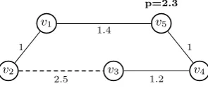
v5

p=2.3

v1

v2 v3 v4

1 1

2.5 1.4

1.2

Figure 1: Segment of a PCSTP instance; edge{v2, v3} (dashed) can be eliminated by the SDC

test.

For the second test some groundwork is necessary. We wish to obtain for a given α∈N to

each terminal itsα d-nearest terminals. Duin’s nearest terminals algorithm allows to compute a constant number ofd-nearest terminalsvi,1, vi,2, ...to each non-terminalvi, but not to terminals.

Remedy is provided by the following lemma. For ease of presentation, we subsequently assume for each{vj, vk} ∈δ N(ti)thatvj∈N(ti) holds.

Lemma 4. Let α ∈ N,1 ≤ α < |T|, ti ∈ T and assume that for each vj ∈ V \T the α+ 1 d-nearest terminalsvj,1, vj,2, ..., vj,α+1 exist and theird-distances toti are available. Thereupon,

settingt(0)_i :=ti, the remainder of theα+ 1d-nearest terminalst(1)_i , ..., t(_iα)totican be computed as follows:

Set t(1)_i :=vk,1 withk such that:

d(ti, vk,1) = min {vj,vk}∈δ(N(ti))

{d(ti, vj) +c{vj,vk}+d(vk, vk,1)}. (7)

Having computedt(1)_i , ..., t(_ir)(r < α), we set t(_ir+1):=vk,l withk, l such that:

d(ti, vk,l) = min

{vj,vk}∈δ(N(ti))

d(ti, vj) +c{vj,vk}

+ min{d(vk, vk,l)|l= 1, ..., r+ 2 :vk,l6=t(_iq), q= 0, ..., r} . (8)

Proof. First, note that both of the minima attained in (7) and (8) correspond to a path. Next, let t(1)_min ∈ T \ {ti} such that d(ti, t(1)_min) is minimal. The corresponding path between ti and

t(1)_min contains an edge{vj, vk} ∈δ(N(ti)) and since the path is of minimumd-length its cost is

d(ti, vj) +c{vj,vk}+d(vk, vk,1). Hence:

min

{vj,vk}∈δ(N(ti))

{d(ti, vj) +c{vj,vk}+d(vk, vk,1)} ≤d(ti, t

(1)

min).

Furthermore, for{vj, vk} ∈δ(N(ti)) letQbe a path consisting of a shortest path betweentiand vj, the edge {vj, vk} and a shortest path betweenvk and vk,1. Sincevj lies in N(ti) and vk,1 is

ad-nearest terminal tovk, the pathQcontains no intermediary terminal vertices. Consequently

it is of cost at leastd(ti, vk,1), so:

min

{vj,vk}∈δ(N(ti))

{d(ti, vj) +c{vj,vk}+d(vk, vk,1)} ≥d(ti, vk,1)≥d(ti, t

(1)

The validity of the claim for r > 1 can be demonstrated similarly: Denote by t(_minr) the

r’th d-nearest terminal to ti, if such a terminal exists. Let r ∈ N,1 < r < α and assume

that there is a t(_minr+1). Additionally, let Q be a path corresponding to d(ti, t(_minr+1)). This path contains an edge{vj, vk} ∈δ(N(ti)) and can therefore be dissected into the subpath Q(ti, vj), the edge {vj, vk} and the subpath Q(vk, t_min(r+1)). The first subpath is of length d(ti, vj), since otherwise it could be substituted by a shorter one. The second subpath is of length at least min{d(vk, vk,l) |l = 1, ..., r+ 2 : vk,l 6= t(_iq), q = 0, ..., r,}, because this is the minimum length betweenvk and a terminal other thant

(0)

i , t

(1)

i , ..., t

(r)

i and without intermediary terminals. Note

thatvk itself can be a terminal, so just scrutinizing allvk,lwithl∈ {1, ..., r+ 1}is not sufficient,

since theser+ 1 terminals could be identical tot(0)_i , t(1)_i , ..., t(_ir). This discussion implies:

min

{vj,vk}∈δ(N(ti))

d(ti, vj) +c{vj,vk}

+ min{d(vk, vk,l)|l= 1, ..., r+ 2 :vk,l6=t(_iq), q= 0,1, ..., r}

≤d(ti, t(_minr+1)).

To see the converse, note that each path Qassociated with the set in (8) is composed of the componentsQ(ti, vj),{vj, vk} andQ(vk, vk,l), for somel such that vk,l∈ {/ t(0)_i , t(1)_i , ..., t(_ir)}. By construction none of these components contain intermediary terminals, thus the same holds for

Q. Hence,C(Q)≥d(ti, vk,l) and therefore:

min

{vj,vk}∈δ(N(ti))

d(ti, vj) +c{vj,vk}

+ min{d(vk, vk,l)|l= 1, ..., r+ 2 :vk,l6=t(_iq), q= 0,1, ..., r}

≥d(ti, t(_minr+1)).

Consequently, the lemma is established.

Corollary 5. Let α ∈ _N, 0 < α < |T|. The α d-nearest terminals to each terminal can be computed with worst-case complexity ofO(m+nlogn)ifαis considered a constant.

Having established Lemma 4, we are in a position to propose a test that scrutinizes alternative paths with up to two intermediary terminals: We compute the four d-nearest terminals (or as many as exist) to each non-terminal vi. For each terminal ti we compute, three d-nearest terminalst(1)_i , t(2)_i , t(3)_i . Additionally, we determine a further terminalt(4)_i that is not necessarily fourthd-nearest toti, but reasonably close empirically. The reason behind this procedure is that for an exact computation the fifthd-nearest nearest terminalsvj,5 to all Steiner verticesvj are

necessary. We proceed by choosing to eachti a terminal vk,l such that:

d(ti, vk,l) = min

{vj,vk}∈δ(N(ti))

d(ti, vj) +c{vj,vk}

+ min{d(vk, vk,l)|l= 1, ...,4 :vk,l6=t(_iq), q= 0,1, ...,3} .

For all (both non-terminal and terminal) verticesvi we denote the set of the so obtained (up to four) close terminals byLi. Next, we scrutinize each edge{vi, vj} ∈E:

Mark each vertex tq ∈Li satisfyingd(vi, tq)< c{vi,vj}. Thereafter, proceed for eachtl∈Lj

such thatd(vj, tl)< c{vi,vj}as follows. Iftlhas been marked andd(vi, tl)+d(vj, tl)−ptl< c{vi,vj},

delete{vi, vj}. Otherwise, if at

(r)

vi andvj, containing exactly two intermediary terminals, namelytl andt(_lr). Next, we examine whether the prize-collecting Steiner distance of this path is smaller than the cost of the edge {vi, vj}. For this purpose, we need to check whether the four inequalities

1. d(tl, t(_lr))< c{vi,vj},

2. d(tl, t(_lr)) +d(vj, tl)−pt_l< c{vi,vj},

3. d(tl, t(_lr)) +d(vi, t(_lr))−p_t(r)

l

< c{vi,vj},

4. d(tl, t(_lr)) +d(vj, tl) +d(vi, t(_lr))−pt_l−p_t(r)

l

< c{vi,vj}

are satisfied. If this is the case, c_{vi,vj} > s(vi, vj) holds and we consequently remove {vi, vj}.

The above procedure is reiterated vice versa, starting from vj and marking all vertices in Lj

to detect additional vi−vj paths containing exactly two intermediary vertices. We name the

described testBottleneck Steiner Distance (SD) test. Since the up to four close terminals are readily available, the foregoing examination of an edge can be performed in constant time. Therefore, these examinations can be accomplished for all edges in a total of Θ(m). Consequently, the SD test can be realized with worst-case complexity ofO(m+nlogn). With upper bounds on the bottleneck Steiner distances being available, we can now also implement a test to Lemma 3: Whenever the test condition is satisfied for avi ∈V \T, this vertex and all incident edges can be discarded, while for each two vertices vk and vj adjacent to vi an edge {vk, vj} with cost

c{vi,vk} +c{vi,vj} is inserted. In the case of two parallel edges, only one of minimum cost is

retained. Analogously to the SPG [11], we call this testNon-Terminal of Degree 3(NTD3). Not only exclusion, but also inclusion tests are possible for the PCSTP: For both the Nearest Vertex (NV) and the Short Links (SL) test for the SPG [30] we propose an extension for the PCSTP, yielding a different but not less powerful result. A somewhat intricate theorem, which may at first glance appear too constraining to be of practical importance, sets the stage.

Initially, a simple procedure is defined that will in the remainder of this section be referred to ascycle-pruning: LetG0= (V0, E0) be a connected subgraph ofG. UntilG0is cycle-free (and therefore a tree), repeatedly select a cycleCG0 and remove an arbitrary edge ofC_G0. It should

be noted that the prize-collecting costC(G0) =P

e∈E0ce+P_v∈V\V0pvofG0is not increased by

this procedure, since only edges are removed, which are by definition of non-negative cost

Theorem 6. Let ti, tj ∈ T, W ⊂ V, with ti ∈ W, tj ∈/ W and |δ(W)| ≥ 2. Further let

e1 ={v1, v10}, e2 ={v2, v02}, withv1, v2 ∈W, be two distinct edges in δ(W) such thatce1 ≤ce2 andce₂ ≤ce˜for alle˜∈δ(W)\ {e1}. Assume that the following three conditions hold:

ce2≥d(ti, v1) +ce1+d(v

0

1, tj), (9)

pt_j ≥d(ti, v1) +ce1+d(v

0

1, tj), (10)

pti≥d(ti, v1) +ce1. (11)

Thereupon, for each feasible solution S toPP C containingti,v1, or v01 (or a combination of

them), there is a solutionS˜ of lesser or equal cost containingti and the edgee1={v1, v10}.

Proof. Let S = (VS, ES) be feasible solution to PP C. Furthermore, for this proof it will be

assumed that cycle-pruning does not remove the edgee1.

In the remainder of this proof three major cases will be differentiated, the first one being

ti∈VS, the secondv1∈VS and the thirdv10 ∈VS. It will be demonstrated that in each of these

three cases there is a solution ˜S that includes bothti and the edgee1={v1, v01} and moreover

i) Supposeti∈VS, but{v1, v10}∈/ ES. Iftj ∈VS, there is a unique path inSbetweentiandtj

that contains an edge{w, w},w∈W,w /∈W of cost at least ce₂. Removing{w, w}one obtains a treeS1 containingti and a treeS2 containingtj. By including a shortest pathQ1 betweenti

and v1 as well as a shortest pathQ2 betweenv10 andtj and including the edge {v1, v10}, a new

subgraph ˜S is obtained. However, ˜S is not necessarily a tree, sinceQ1◦ or Q2◦ may contain a

vertex ofS, resulting in a cycle. In this case, ˜S is modified by applying cycle-pruning. Thereby, ˜

S is rendered a tree and, containingVS, it is of cost:

C( ˜S)≤C(S)−ce2+d(ti, v1) +ce1+d(v

0 1, tj)

(9)

≤ C(S).

In the complementary casetj ∈/ VS, construct a tree ˜S by once again includingQ1 andQ2 and

inserting the edge{v1, v01}, followed by cycle-pruning. The tree ˜S is of cost:

C( ˜S)≤C(S) +d(ti, v1) +ce1+d(v

0

1, tj)−ptj

(10)

≤ C(S).

ii) Supposev1∈VS. Ifti∈/VS, then by adding a shortest path betweenti and S a tree ˜S of

cost:

C( ˜S)≤C(S)−pti+d(ti, v1)

(11)

≤ C(S)

is obtained. Since ti ∈ S˜, one can proceed as in case i) to find a tree ˜S0 with C( ˜S0) ≤ C( ˜S) that contains bothti and {v1, v10}. Finally, if ti∈VS holds in the first place, one can forthwith

procced as in case i).

iii) Supposev01∈VS. Ifti∈VS but{v1, v10}∈/ ES, there is a unique path inSbetweenv10 and

ti that contains an edge{w, w}, w∈W, w /∈W of cost at leastce2. The tree ˜S obtained from

S by removing {w, w} and inserting e1={v1, v10} as well as including a shortest path between

v1 andti (and if necessary performing cycle-pruning) is of cost:

C( ˜S)≤C(S) +ce1+d(v1, ti)−ce2

(9)

≤C(S).

On the other hand, consider the caseti∈/VS. The addition of a shortest path betweenv1andti

and the addition of the edgee1(if not already present) connectsti to S. After cycle-pruning, a

tree ˜S of cost:

C( ˜S)≤C(S) +ce₁+d(v1, tj)−pti

(11)

≤ C(S)

is obtained.

Contrary to the NV and SL tests for the SPG, in the case of the PCSTP one cannot assume that{v1, v01}is part of at least one minimum Steiner tree. However, the following corollary allows

us to contract the edge nevertheless. Initially, consider a PCSTPP_{P C}0 resulting from contracting an edge of a PCSTP PP C. Thereupon, a solution to P_{P C}0 may correspond to several solutions to PP C. In the following it is presupposed that in such a case among these solutions one of minimum cost is selected.

Corollary 7. Assume that the premises of Theorem 6 are fulfilled and furthermore that inequality (11) holds strictly or v1 =ti is satisfied. Let PP C0 = (V0, E0, c0, p0) be the PCSTP obtained by

contracting e1 ={v1, v01} in the following way. If bothv1 =ti andv10 =tj, contractv01 into vi

and setp0_t

i:=pti+ptj−ce1. Otherwise, definep

0

ti:=pti−ce1 and contractv1 intov

0

1 ifv01=tj

or contract v0₁ intov1 if v10 6=tj. In each case setp0v:=pv for allv∈V0\ {ti}.

Thereupon, for each optimal solution S0 toP_{P C}0 the corresponding solution S toPP C is also

Proof. LetS0 = (V_S00, E_S00) be a solution toP_{P C}0 and S = (VS, ES) the corresponding solution

to PP C. The cost of S0 (with respect to P_{P C}0 ) is denoted byC0(S0). Additionally, assume that

e1 = {v1, v10} is contracted into v1 (the opposite case is analogous). Initially, two cases are

discussed, namely i)v1, ti∈/VS00 and ii)v1, ti∈VS00.

i) Assumev1, ti ∈/ VS00. In this caseS0 andS consist of exactly the same edges and vertices,

which implies that P e∈E0

S0c

0

e = P

e∈ESce. Recall that if bothv1 =ti and v

0

1 =tj hold, then

p0_ti =pt_i+pt_j −ce₁ and otherwise p0_ti =pt_i−ce₁. Thereupon, it can be further inferred that

P v /∈V0

S0p

0

v = P

v /∈VSpv−ce1. These deliberations amount to the equation:

C0(S0) +ce₁=C(S). (12)

ii) Assume v1, ti ∈ VS00. Consequently, P

e∈E0

S0c

0

e +ce1 =

P

e∈ESce and

P v /∈V0

S0p

0

v = P

v /∈VSpv hold, so:

C0(S0) +ce₁=C(S). (13)

In the following assume that S0 is an optimal solution toP_{P C}0 . In this case, one can verify that only the two cases i) and ii) discussed above can occur. This assertion is certainly true if ti = v1, since in this case it can only hold that either v1, ti ∈/ VS00 or v1, ti ∈ VS00. In the

following it will therefore be assumed thatti6=v1. Consequently, according to the conditions of

this corollary, inequality (11) holds strictly, i.e. pti > d(ti, v1) +ce1 is satisfied. Once more, two cases need to be considered.

First, suppose ti ∈VS00 andv1∈/ VS00. This implies for the corresponding solution S to PP C

that ti ∈VS andv1∈/ VS. Consequently, it holds that Pe∈E0

S0

c0_e=P

e∈ESce and

P v /∈V0

S0

p0_v=

P

v /∈VSpv, soC

0_(S0_{) =C(S). Furthermore, according to Theorem 6 there would a solution ˜S to}

PP Cof cost C( ˜S)≤C(S) that containsti,v1, andv10. Due to case i) the corresponding solution

˜

S0 toP_{P C}0 would be of costC( ˜S)−ce, so one could infer that:

C0(S0) =C(S)≥C( ˜S) =C0( ˜S0) +ce> C0( ˜S0),

which contradicts the assumption thatS0 is optimal.

Conversely, supposeti ∈/ V_S00 andv1∈VS00. Sincept_i> d(ti, v1) +ce1 is satisfied,S

0 _{could be}

connected toti, in the graph (V0, E0), by a path of cost at most

d(v1, ti)< pti−ce1 =p

0

ti,

which would give rise to a solution of smaller cost.

Based on the above discussions, one can finally prove the corollary. To this end, letS0 be an optimal solution toP_{P C}0 . Thereupon, it needs to be demonstrated thatS is an optimal solution toPP C. Suppose this is not true, i.e. that there is a solution ˆSto PP C such thatC( ˆS)< C(S). According to Theorem 6, it may be assumed that ˆS contains either ti, v1, and v01 or none of

them. Due to (12) and (13), in both cases the corresponding solution ˆS0toP_{P C}0 would be of cost

C0( ˆS0) =C( ˆS)−ce< C(S)−ce=C0(S0),

contradicting the assumption thatS0 is optimal. Concludingly,S has to be an optimal solution toPP C.

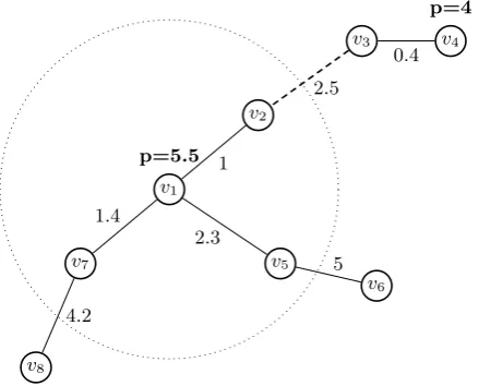
v1

p=5.5

v4

p=4

v7

v3

v2

v5

v6

v8

2.3

5 1

2.5

1.4

4.2

0.4

Figure 2: Segment of a PCSTP instance; settingW :={v1, v2, v5, v7}, one infers from Corollary 7

that edge{v2, v3} (dashed) can be contracted.

Lemma 8. Let W ⊂V andti∈W,tj ∈/ W. Ifδ(W) =∅,W∩T ={ti} andpt_j ≥pt_i, there is an optimal solutionS?_{= (VS?, ES?)withVS?∩W =∅. Ifδ(W) ={e}

1}, where ={e1}={v1, v01}

andv1∈W, and moreover the conditions (10)and (11)of Lemma 6 hold, then for each feasible

solution S toPP C containingti,v1, or v01 (or a combination of them), there is a solutionS0 of

lesser or equal cost containing bothti and the edge e1={v1, v01}.

With those rather general results at hand, we are now able to formulate extended forms of the NV and the SL test for the PCSTP.

Lemma 9. Let ti be a terminal of degree at least 2 and let e0i ={ti, vi0} and e00i ={ti, vi00} be a

shortest and a second shortest incident edge. Assume that there is a terminal tj6=ti such that:

ce00

i ≥ce0i+d(v

0

i, tj), (14) pt_j ≥ce0

i+d(v

0

i, tj), (15)

pti ≥ce0_i. (16)

Thereupon, for each feasible solutionStoPP C containingtiorvi0, there is a solutionS0 of lesser

or equal cost containing{ti, v0i}.

Proof. DefiningW :={ti}, one can identify the lemma as a special case of Theorem 6.

Condition (14) of Lemma 9 can be verified analogously to the NV test for the SPG [30] in

O(m+nlogn). Furthermore, withd(v0_i, tj) available, the additional conditions (15) and (16) can be verified trivially by checking all incident edges ofti. Since each edge is thereby checked at most twice, this can be rendered for the entire set of terminals in Θ(m). Additionally, the test can be extended based on the subsequent lemma.

a terminaltj 6=ti such that:

ce≥ce0

i+d(v

0

i, tj) for all e∈δ({ti, v00i})\ {e0i}, (17) pt_j ≥ce0

i+d(v

0

i, tj), (18)

pti≥ce0_i, (19)

then for each feasible solutionS toPP C containing ti or v_i0, there is a solution S0 of lesser or equal cost containing{ti, v0i}.

Proof. DefiningW :={ti, v_i00}, one can identify the lemma as a special case of Theorem 6.

In the context of the PCSTP, we call the test associated with Lemma 9 and Lemma 10 that contracts edges as described in Corollary 7 by Nearest Vertex (NV) test. Since Lemma 10 can be realized with additional costs ofO(m), NV is ofO(m+nlogn).

Theorem 6 can furthermore be used to verify the following two lemmata, which in turn set the stage for a Voronoi based inclusion test.

Lemma 11. Let ti be a terminal and let e01 = {v1, v10} ande02 ={v2, v02} be a shortest and a

second shortest Voronoi-boundary edge of N(ti) (satisfying v1, v2 ∈ N(ti) and v01, v20 ∈/ N(ti)).

Let tj :=base(v02)and assume:

ce0

2≥d(ti, v1) +ce

0

1+d(v

0

1, tj), (20)

pt_j ≥d(ti, v1) +ce0

1+d(v

0

1, tj), (21)

pti≥d(ti, v1) +ce01. (22)

Then for each feasible solutionS toPP C containingv1 orv10, there is a solutionS0 of lesser or

equal cost containing{v1, v10}.

Proof. DefiningW :=N(ti), one can identify the lemma as a special case of Theorem 6.

Lemma 12. Let ti be a terminal and let e01:={v1, v10} be a shortest Voronoi-boundary edge of

N(ti). Assume that there is a second Voronoi-boundary edge of N(ti), namely e02 = {v2, v20},

withv0

2∈/ T∪ {v01}. Further, lettj :=base(v20)and assume:

ce≥d(ti, v1) +ce0

1+d(v

0

1, tj), ∀ e∈δ({ti, v00i})\ {e01}, (23)

pt_j ≥d(ti, v1) +ce0

1+d(v

0

1, tj), (24)

pti≥d(ti, v1) +ce01. (25)

Then for each feasible solutionS toPP C containingv1 orv10, there is a solutionS0 of lesser or

equal cost containing{v1, v10}.

Proof. DefiningW :=N(ti)∪{v₂0}, one can identify the lemma as a special case of Theorem 6.

We denote the test associated with Lemma 11 and Lemma 12 that contracts edges as described in Corollary 7 by Short Links(SL). Additionally, this test checks whether the conditions of Lemma 8 are satisfied. SL can be realized inO(m+nlogn): The computation of the Voronoi diagram requiresO(m+nlogn) [28] and a shortest and second shortest Voronoi-boundary edge to all terminals can be computed by traversing all Voronoi region, in a total of Θ(m). The extension of the test affiliated with Lemma 12 is restricted to terminals ti such that |δ(ti)| ≥

2∗ |δ(v_i00)|, bounding the additional costs toO(m). Note that the distancesd(v1, ti) andd(v10, tj)

2.3

Bound-Based Reductions

This section describes a series of reduction methods that identify edges and vertices ofPP C for elimination by examining whether they induce a lower bound that exceeds a given upper bound. Two classed of tests will be discussed. The first type is based on the concept of the Voronoi diagram (2), the second one on a fast dual-ascent heuristic.

2.3.1 Voronoi Diagram Tests

For the SPG, bound-based methods can be built upon the radiusconcept that was introduced in [30]. Given a Voronoi diagramN and a terminalti∈T,radius(ti) is defined as the minimum cost of any path containingti and leavingN(ti) [30]. This concept can be generalized for the (R)PCSTP as follows:

pcradius(ti) := min{radius(ti), pti}, ti∈T. (26)

The adaptation of the radiusdefinition is necessary because a feasible solution to an SPG contains for each Voronoi region a path that leaves this region, whereas this assumption does not hold for the (R)PCSTP—since feasible solutions to the (R)PCSTP do not need to contain all ter-minals. Definition (26) sets the stage for a series of lemmata and corollaries presented hereinafter that allow to eliminate both vertices and edges. For ease of understanding, it is presupposed that all terminals are ordered such thatpcradius(t1)≤pcradius(t2)≤... ≤pcradius(ts). The

first lemma can be seen as an extension of a test already known for the SPG [30]. The reader is reminded that we have defineds:=|T|.

Lemma 13. Letvi∈V \T. If a minimum Steiner treeS= (VS, ES)with vi∈VS exists, then

d(vi, vi,1) +d(vi, vi,2) +P

s−2

q=1pcradius(tq)is a lower bound on the cost ofS.

Proof. Assume that there is a minimum Steiner tree S = (VS, ES) such that vi ∈VS. Denote

the (unique) path in S between vi and a terminal tj ∈VS byQj and the set of all such paths byQ. First, note that |Q| ≥2, because ifQjust contained one path, say Ql, the single-vertex tree{tl} would be of smaller cost thanS, contradicting the initial assumption that the latter is of minimum cost. Second, if a vertex vk is contained in two distinct paths inQ, the subpaths of these two paths between vi and vk coincide. Otherwise there would need to be a cycle inS. Additionally, there are at least two paths inQhaving only the vertexvi in common. Otherwise, due to the precedent observation, all paths would have one edge{vi, v_i0}in common which could be discarded, yielding a tree of smaller cost thanS.

Now, choose two distinct paths Qk ∈ Q and Ql ∈ Q such that their combined number of Voronoi-boundary edges is minimal and V[Qk]∩V[Ql] = {vi} holds. Further, define Q− _:=

Q \ {Qk, Ql}. For allQr∈ Q−, denote byQ0rthe subpath ofQr betweentrand the first vertex

not in N(tr). Suppose that Qk has an edge e ∈ ES in common with a Q0r: Consequently, Ql

cannot have any edge in common withQr, because this would require a cycle inS. Furthermore,

according to the preceding observations,QkandQrhave to contain a joint subpath includingvi

ande. But this would imply that Qk contained at least one additional Voronoi-boundary edge

(in order to be able to reachtk, which is by definition not inN(tr)). Therefore, and due toQl

andQrbeing edge disjoint,Qrwould have initially been selected instead ofQk.

combined cost, one can obtain a lower bound on the cost ofS by:

C(S) = X

e∈ES

ce+ X

v∈V\VS

pv

≥

X

Qr∈Q−

C(Q0r)

+C(Qk) +C(Ql) + X

v∈V\VS

pv

≥

s−2

X

q=1

pcradius(tq) +C(Qk) +C(Ql)

≥

s−2

X

q=1

pcradius(tq) +d(vi, vi,1) +d(vi, vi,2)

whereC(Q) :=P

e∈E[Q]ce. Ergo, the lemma is proven.

A Steiner vertex vi can be discarded if its associated lower bound, specified in Lemma 13, exceeds a known upper boundU of the underlying problem. If a solutionSof costU is available,

vi can eliminated in the case of equality of both bounds if additionally vi ∈/ V[S] is satisfied. Analogous tests are possible for all subsequent lemmata and corollaries in this subsection.

A similar approach can be applied to probe whether a terminal is part of any optimal solution. Recall that to each terminalti we denote byt(1)_i 6=ti a terminal of shortest distance toti.

Corollary 14. Let ti ∈ T and assume that a minimum Steiner tree S = (VS, ES) other than

{ti} exists such that ti ∈VS. Additionally, let φ:{1, .., s} → {1, .., s} be a bijection, such that φ(i) = 1 and all tφ(j) are ordered such that the pcradius(tφ(j)) values are non-decreasing in

j= 2, ..., s. In this case,d(ti, t(1)_i ) +Ps−1

q=2pcradius(tφ(q))is a lower bound on the cost of S.

If a terminal cannot be eliminated using the conditions of the antecedent corollary, another approach based on the following lemma can be attempted:

Lemma 15. Let ti ∈ T and assume that a minimum Steiner tree S = (VS, ES) exists such

that ti is of degree at least 2 in S. Additionally, letφ:{1, .., s} → {1, .., s} be a bijection, such

thatφ(i) = 1 and alltφ(j)are ordered such that the pcradius(tφ(j))values are non-decreasing in

j = 2, ..., s. In this case, d(ti, t(1)_i ) +d(ti, t(2)_i ) +Ps−2

q=2pcradius(tφ(q))is a lower bound on the

cost of S.

The last lemma can be utilized to show that in all optimal solutions the terminalti is either

not contained or of degree 1. To make use of this information, the following simple reduction test can be applied.

Lemma 16. Let ti∈T and assumept_i ≤ce for alle∈δ(ti). Ifti is not contained or of degree 1 in at least one minimum Steiner tree, there exists a minimum Steiner tree not containingti.

If the premises of Corollary 14 or Lemma 16 are fulfilled, ti and all incident edges can be deleted. To obtain the original solution value, pt_i needs to be added to the objective value of each feasible solution (analogously to the TD0 test).

Lemma 17. Let {vi, vj} ∈ E. If there is a minimum Steiner tree S = (VS, ES) such that

{vi, vj} ∈ES, thenL defined by

L:=c{vi,vj}+d(vi, vi,1) +d(vj, vj,1) +

s−2

X

q=1

ifbase(vi)6=base(vj)and

L:=c_{vi,vj}+ min

d(vi, vi,1) +d(vj, vj,2), d(vi, vi,2) +d(vj, vj,1)

+

s−2

X

q=1

pcradius(tq) (28)

otherwise, is a lower bound on the cost ofS.

Lemma 18. Let vi∈V \T, δ(vi)≥3. If there exists a minimum Steiner treeS such that vi is of degree at least3 in S, thend(vi, vi,1) +d(vi, vi,2) +d(vi, vi,3) +P

s−3

q=1pcradius(tq)is a lower

bound on the cost ofS.

Occasionally, an even stronger bond can be obtained by utilizing the following lemma, which can be seen as a generalization of a lemma introduced in [30].

Lemma 19. Let G0 = (T, E0) be graph in which two vertices ti and tj (which correspond to terminals in G) are adjacent if and only if there is an edge{v, w} ∈E such that v∈N(ti)and

w∈N(tj). Additionally, define a cost functionc0 on E0 by

c0_{ti,tj}:= min{min{pt_i, pt_j, d(ti, vi), d(tj, vj)}+c{vi,vj} |vi∈N(ti), vj ∈N(tj)}.

The weight, with respect toc0, of a minimum spanning tree forG0 is a lower bound on the weight of any Steiner tree for (V, E, c, p)

All antecedent bound-based tests can be easily modified to make use of the bound obtained from Lemma 19. For instance, one may adapt Lemma 17 by substituting the value L by the weight of a minimum spanning tree forG0 minus the weight of its longest edge (analogously to the procedure for the SPG described in [30]).

The test associated with the introduced bound-based reduction approaches is denoted by

Bound (BND) test. It works with an upper bound computed by a constructive heuristic that was introduced in [17]. The worst-case complexity, which would otherwise be ofO(m+nlogn), is dominated by the constructive heuristic, which exhibits a complexity ofO(s(m+nlogn)) but is empirically very fast.

2.3.2 Dual-Ascent Tests

For the final bound-based test we transfer a powerful reduction technique for the Steiner tree problem in graphs, thedual-ascent method[11, 30]. While this method is a bound-based reduction test, it is distinctively different from the bound-based methods previously introduced in this paper.

To set the stage, we first define the Steiner arborescence problem (SAP): Given a directed graphD= (V, A), costsc:A→Q≥0, a setT ⊆V of terminals and a rootr∈T, a directed tree

(arborescence)S = (VS, AS)⊆D of minimum costPa∈ASca is required such that for allt∈T

the treeS contains a directed path fromrto t.

Considering an SAP (V, A, c, r), we associate with each arc a ∈ A a variable ya indicating

whether ais contained in the Steiner arborescence (ya = 1) or not (ya = 0). Thereupon, an IP formulation can be stated as [36]:

Formulation 1. Directed Cut Formulation

min cTy (29)

y(δ−(W)) ≥ 1 for all W ⊂V, r /∈W, W ∩T 6=∅, (30)

In [36] a dual-ascent algorithm for the SAP was introduced that, empirically, both provides strong lower bounds and allows for fast computation, defying its worst-case time complexity ofO(|E|min{|V||T|,|E|}) [30]. Efficient implementations of the algorithm can be found in [11] and [29]. We use the latter implementation combined with the heuristic guiding-solution criterion suggested in [30]. At termination, dual-ascent provides a dual solution to the LP relaxation of Formulation 1, involving directed paths along arcs with a reduced cost of 0 from the root to each additional terminal. This information can be used for the SPG reduction method dual-ascent [11, 30], which is based on the possibility to transform the SPG to the SAP, see for instance [32].

In the following we demonstrate the dual-ascent approach for the RPCSTP, but it can be naturally extended to the PCSTP and MWCSP. The first step is to transform a given RPCSTP to an SAP, as we already described in [33]:

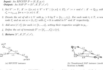
Transformation 1(RPCSTP to SAP).

Input: An RPCSTPP = (V, E, p, r) Output: An SAPP0= (V0, A0, T0, c0, r0)

1. Set V0 := V, A0 := {(v, w) ∈ V0 ×V0 | {v, w} ∈ E}, r0 := r and c0 : A0 → Q≥0 with

c0_a=c{v,w} fora= (v, w)∈A0.

2. Denote the set of allv ∈V with pv >0 by T ={t1, ..., ts}. For each node ti ∈T, a new

nodet0_i and an arc a= (ti, t0_i)with c0_a= 0 is added toV0 andA0 respectively.

3. Add arcs(r0, t0_i)for each i∈ {1, ..., s}, setting their respective weight topti.

4. Define the set of terminalsT0 :={t01, ..., t0s} ∪ {r}.

5. Return (V0, A0, T0, c0, r0).

r

p=2.5 p=7

1.2

2.3 1.6

1 1.3

1.5

(a) RPCSTP instance

r 1.2 2.3

1.6

1 1.3

1.5 2.5 7

0 0

(b) Transformed SAP instance (modi-fications inbold)

Figure 3: Illustration of an RPCSTP instance with rootr(left) and the equivalent SAP obtained by Transformation 1 (right). Terminals are drawn as squares and Steiner vertices as circles (with those of positive weight enlarged).

Lemma 20(RPCSTP to SAP). Let P0 = (V0, A0, T0, c0)be an SAP obtained from an RPCSTP

P = (V, E, c, p)by applying Transformation 1. Each solutionS0= (V_S00, A0_S0)toP0can be mapped

to a solutionS = (VS, ES)toP defined by:

VS:={v∈V |v∈V_S00} (32)

ES :={{v, w} ∈E|(v, w)∈A0S0 or(w, v)∈A0_S0} (33)

With this transformation at hand, let vi ∈V /T and S? _{be an optimal Steiner arborescence}

to a given SAP instance (V, A, c, r) and LDA the lower bound obtained by dual-ascent. If S?

containsvi, the weight ofS? _{can be bounded from below byLDAplus the length (with respect}

to the reduced costs provided by dual-ascent) of a shortest path from the root to vi and the length of a shortest path from vi to ad-nearest terminal (other than the root) tovi. Hence, vi

can be deleted if the just defined bound exceeds a known upper bound U. An analogous test can be stated for the elimination of arcs. Since each RPCSTP instance can be transformed to an SAP, the above deliberations forthwith set the stage for an RPCSTP reduction technique: Whenever a vertex can be deleted in the SAP, the same is true for its counterpart in the analogous RPCSTP. Similarly, if two anti-parallel arcs of the SAP have been shown to be removable, the corresponding edge of the RPCSTP can be discarded. Finally, a test to replace vertices by edges that is analogous to NTDk can be used.

In addition to these methods already known for the SPG, the graph transformation from RPCSTP to SAP sets the stage for two new tests. First, terminals of the RPCSTP can be deleted if the corresponding vertex ti in the SAP is shown to be removable. Second, if the

reduced cost of an arc (r0, t0_i) is higher thanU −LDA, we can deduce that the vertexti is part of an optimal solution toP. Consequently, we can set its prize to infinity, which possibly allows several tests (such as SDC) to perform additional reductions. Moreover, we can create a new SAP usingti as the root, which can pave the way for additional eliminations by the above procedure. In our reduction package the maximum number of root changes and subsequent dual-ascent runs is limited to 15.

As with the BND test, all dual-ascent based reduction methods can be extended to the case of equality if a Steiner tree corresponding to the upper bound U is given. We call the entire procedure of computing the reduced costs on the SAP, computing an upper bound to the original problem and eliminating vertices and edges as well as fixing terminalsDual-Ascent(DA) test. Obviously, one question remains, namely how to obtain an upper bound for the DA test. As will be shown in the following, the availability of the reduced costs provided by DA allows to transfer an heuristic approach already known for the SPG.

Ascend-and-Prune

Theascend-and-prune heuristic has been demonstrated to be a powerful device for the Steiner tree problem in graphs [30]. An extension of the heuristic to the (R)PCSTP (and the MWCSP) was essentially impeded by the lack of two techniques: Transformations of (R)PCSTP and MWCSP to SAP and powerful reduction methods. With both transformations and strong re-duction techniques at hand, the ascend-and-prune approach can be extended beyond the SPG.

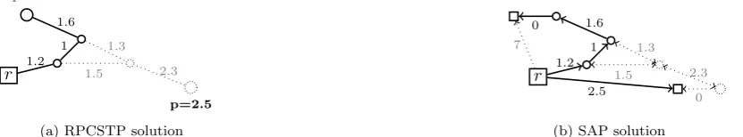
Let P be the original RPCSTP and P0 the SAP resulting from Transformation 1. The

r

p=2.5

p=7

1.2

2.3

1.6

1 1.3

1.5

(a) RPCSTP solution

r 1.2 2.3

1.6

1 1.3

1.5

2.5

7

0

0

(b) SAP solution

ascend-and-prune heuristic attempts to find a good solution on the subproblem ˜P constituted by the undirected edges of P corresponding to zero-reduced-cost paths in P0 from the root to all additional terminals. This approach is motivated by the assumption that notable similarities exist between an optimal (or nearly optimal) Steiner tree and the LP solution corresponding to the reduced costs provided by dual-ascent.

To find a solution to ˜P, the concept of the prune heuristic [30] for the SPG is transfered to the RPCSTP. This extension is possible by virtue of the new reduction tests, in particular BND, introduced in this paper. The heuristic works as follows: After applying all previously introduced reduction techniques on ˜P, we use an heuristic extension of the BND test to further reduce ˜P. While for the original BND test the upper bound is provided by a primal solution, in the prune heuristic the bound is decreased in such a way that in each iteration a constant amount of edges and vertices is eliminated. Thereupon, all (exact) reductions methods are executed on the reduced problem, motivated by the assumption that the (possibly inexact) eliminations performed by the bound-based method will allow for further reductions. This procedure is reiterated until not more than two terminals remain. To avoid infeasibility, we compute a Steiner tree by using the shortest path constructive heuristic described in [32] and forbid eliminations of any of its vertices or edges by the inexact BND test. In [33] we implicitly used the previously described reduction techniques to implement ascend-and-prune for the (R)PCSTP and MWCSP and demonstrated its ability to find strong, often optimal upper bounds within short time.

2.4

Reiteration and Ordering

Studying different combinations and orderings of reduction techniques, we have come to the conclusion that the tests are not overly sensitive to the order of their execution (as with the SPG [30]). However, this is not true for the total reduction time.

The underlying precept for the ordering of the reduction methods is to perform the faster ones first so that the more expensive tests are applied to, hopefully, substantially reduced graphs. Furthermore, it seems reasonable to perform the two SD test variants prior to the NTD3 test,

since the former reduces, if successful, the degrees of vertices. Additionally, first performing the SD test allows us to reuse the computed d-distances for the NTD3 test. Similarly, due to the

NTD3and SD variant tests deleting edges (and possibly replacing pairs of edges by a single one),

they are performed prior to the NV and SL tests.

All reduction tests are arrayed in a loop that is reiterated as long as a constant proportion (for our solver 0.5 percent) of edges were eliminated during the last run. Thereby, one obtains the same asymptotic time bound as the most expensive performed reduction test; due to DA this bound is of O(|E|min{|V||T|,|E|}). This bound implies in particular that the reduction package is of polynomial worst-case complexity. Furthermore, during a succeeding loop each test is performed only if it could eliminate a constant proportion (0.1 percent) of edges during the previous run. Moreover, the BND test is executed only if at most three percent of all vertices are terminals; we have observed that the test is otherwise of very little effect.

Additionally, we have implemented an exhaustive version of the reduction package, in which the loop as well as all tests are reiterated until no more reductions can be performed. This loop is not supposed to be used a preprocessing step for exact solving (unless the instance to be solved is known to be hard), but rather for demonstrating the capacity of the reduction tests.

3

The Maximum-Weight Connected Subgraph Problem

the objective is to find a connected subgraph S = (VS, ES) ⊆G such that P

v∈VSpv is

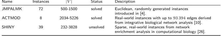
maxi-mized. The problem has been discussed in various publications [4, 10, 20]. Practical applications of the MWCSP can be found in diverse areas such as wildlife conservation [9], computational biology [10] and computer vision [8].

Several publications about the MWCSP have addressed exact solving approaches [4, 5, 13, 14]. However, compared to the SPG very little research has been performed regarding reduction techniques for the MWCSP [3, 13]. This provided an incentive for us to develop various novel techniques, which will be subsequently introduced along with several others known from the literature.

In the following it is assumed that at least one vertex is assigned a negative and one a positive weight. In the case of only non-negative vertex-weights, the problem reduces to finding a connected component of maximum vertex weight; in the case of only non-positive vertex-weights, the empty set constitutes an optimal solution. For a given solutionS= (VS, ES) to an

MWCSP we denote its weight by C(S) :=P

v∈VSpv. Note that to each feasible solution there

is a solution of the same weight that additionally is a tree—such a solution can for example be obtained by the cycle-pruning procedure introduced in Section 2. For simplicity, in the following lemmata it will be assumed that each solution to an MWCSP is a tree.

Furthermore, throughout this section it will be presupposed that an MWCSP instancePM W = (V, E, p) is given. The remainder of the notation is analogous to the one introduced in Section 2.

3.1

Basic Reductions

Analogous to the PCSTP, reductions for vertices of low degree are readily conceived. The first of the following two simple tests was already suggested in a less general form in [13] (namely only for negative vertices of degree 0):

Vertex of degree 0 (VD0): A vertex vi of degree zero can be discarded if there is a vertex

vmax such that bothpv_max≥pv_i and vmax6=vi.

Vertex of degree 1 (VD1): If there is vertex vi of degree 1 with incident edge ek ={vi, vj},

a vertexvmax satisfying bothpv_max≥pv_i andvmax6=vi and it moreover holds that

a) pv_i≤0, thenvi andek can be discarded;

b) pv_i>0, thenvi andek can be discarded while adding pv_i to the weight ofvj.

The next two reduction tests can be found in both [3] and [13].

Non-negative incident vertices (NNIV): An edge {vi, vj} such that pvi ≥0,pvj ≥0 can

be contracted if the weight of the remaining vertex is set topvi+pvj.

Non-positive chain (NPC): A path Q between two vertices vi, vj, containing only

non-positive interior vertices of degree 2 and fulfilling |V[Q]| >3 can be replaced by a node v0 with

pv0 :=P

v∈V[Q◦_]pv and the two edges {v0, vi},{v0, vj}.

The joint execution of the four forgoing tests, in the specified order, will be hereinafter referred to asBasic Test(BT).

Recalling that connectivity is not postulated for the MWCSP, one readily devises the following test:

3.2

Alternative-Based Reductions

Alternative-based reductions for the MWCSP have not been comprehensively researched in the literature yet. This section aims for a more extensive study by introducing many novel reduction techniques, which, to the best of the authors’ knowledge, have not been previously published.

The subsequent reduction test was tentatively suggested in [13], to be later generalized in [3]. Only the latter version is stated here:

Adjacent Neighbourhood Subset (ANS)1 _{Letvi andvj be two distinct vertices. Ifpv}

i≤0,

pv_i ≤pv_j and

v∈V \ {vj} | {vi, v} ∈E ⊆

v∈V | {vj, v} ∈E ,

thenvi and all incident edges can be removed.

However, even this revised version can be notably generalized:

Lemma 21. Let vi ∈ V and W ⊆ V \ {vi}, W 6= ∅ such that (W, E[W]) is connected and P

w∈W:pw<0pw≥pvi holds. If

v∈V \W | {vi, v} ∈E ⊆

v∈V \W | {w, v} ∈E, w∈W (34)

is satisfied, then there is at least one optimal solution that does not containvi.

Proof. Suppose that there is an optimal solutionS= (VS, ES) containingvi. Since

X

w∈W:pw<0

pw≥pvi

it can be inferred thatpv_i≤0. Therefore, it can be assumed thatviis of degree at least 2 in

S(ifviis of degree 1 inS, it can be simply discarded without deteriorating the objective value). Let ∆S ⊂VS be the vertices adjacent to vi in S. Removing vi and all incident edges from S

and inserting all vertices in W\S as well as all edges between W and ∆S∪W, one obtains a

connected subgraphS0= (VS0, ES0) such that:

C(S0) = X

v∈V_S0

pv≥ X

w∈W

pw<0

pw+C(S)−pvi ≥C(S). (35)

Due to (35) it holds thatS0 is optimal. Furthermore, by constructionS0 does not containvi, so the statement of the lemma is established.

Affiliated to Lemma 21 we suggest the subsequent reduction test. For each vertex vj ∈ V

proceed as follows: Define Wj as the union of vj and all non-negative adjacent vertices of vj.

Next, we mark all neighboring vertices ofWj. Finally, we check for all non-positive neighboring vertices vi of Wj such that pv_i ≤ pv_j whether condition (34) holds. If this is the case, vi can be deleted. In the following, this test is referred to as Connected Neighborhood Subset (CNS).

Furthermore, we suggest an extension of CNS for which not only all vi adjacent to Wj but allvi∈V\Wjsuch thatpv_i ≤pv_j are scrutinized. We call this variantAdvanced Connected Neighborhood Subset(ACNS) test.

The perhaps most intuitive, but nonetheless effective, of the reduction tests introduced here-inafter is based on the following lemma:

v5

1.5

v6

-2

v1

-2

v2

-1

v3

4

v4

-1.9

Figure 5: Segment of an MWCSP instance. Lemma 21 guarantees that vertexv1and its incident

edges (dashed) can be eliminated, since each neighbor ofv1 is a neighbor of eitherv5or v6

Lemma 22. Let ek={vi, vj} ∈E. If there is a pathQbetween vi andvj such that ek ∈/ E[Q]

andpv_l≥0 for allvl∈V[Q◦], then there is at least one optimal solution that does not contain

ek.

Proof. Let S be a solution to PM W containing ek. By removing ek from S one obtains two

connected subgraphs S1,S2 such thatvi ∈S1, vj ∈S2. Since Qconnectsvi and vj, there are

vertices vr ∈ V[S1]∩V[Q], vs ∈ V[S2]∩V[Q] such that for the induced subpath Q(vr, vs) it

holds that V[S1]∩V[Q(vr, vs)] ={vr} and V[S2]∩V[Q(vr, vs)] ={vs}. Reconnecting S1 and

S2 byQ(vr, vs) one yields a new connected subgraph ˜S of weight at leastC(S).

These discussions prove the lemma, since they imply that to each solution that contains ek, a solution of greater or equal weight not containingek can be constructed.

We suggest a reduction test based on Lemma 22, designed as follows: By first executing the NNIV test, each path containing only interior vertices of non-negative weight is reduced to a path consisting of three vertices (with an interior vertex of non-negative weight). Thereafter, to probe an edge{vi, vj}it suffices to check all adjacent vertices of bothviandvj. By bounding the

number of adjacent vertices to be visited fromviandvjby a constant, the test can be performed

for all edges in a total of Θ(m). We call this testNon-Negative Paths (NNP).

The development of the next reduction strategy originated from the observation that after the NPC test has been performed each non-positive chain is reduced to a single non-positive vertex of degree 2. Naturally, one aspires to dispose of those as well. To set the stage for such a reduction method we define a function on two vertices, similar to that of the bottleneck Steiner distance: Letvi, vj ∈V be two distinct vertices andQ(vi, vj) the set of all simple paths between

vi andvj. In the context of the MWCSP we define theinterior cost of such a subpath as:

C◦(Q(x, y)) := X

v∈V[Q(x,y)]\{x,y}

pv. (36)

Furthermore, we define thevertex weight bottleneck length ofQas:

ˆ

l(Q) := min

x,y∈V[Q]C

Given two disjoint connected subgraphs that can be connected by a subpath of a given pathQ, by ˆl(Q) a lower bound on the additional vertex weights is provided.

The two preceding definitions pave the way for thevertex weight bottleneck distancebetween

vi andvj that we define as

ˆ

d(vi, vj) := max{ˆl(Q)|Q∈ Q(vi, vj)}. (38)

With this new definition at hand, a lemma bearing some similarities with the Steiner distance based exclusion tests can be formulated.

Lemma 23. Let vi ∈ V such that pvi ≤ 0 and |δ(vi)| = 2 with incident edges {vi, vj} and

{vi, vk}. If

ˆ

d(vj, vk)> pvi (39)

holds, then there is at least one optimal solution not containingvi.

Proof. Suppose that there is an optimal solution S that contains vi. In this case, due to vi

being of non-positive weight, we can assume that both incident edges of vi are likewise part of

the solution. Otherwise, vi could simply be removed, yielding another optimal solution (or a

solution greater weight, which would forthwith contradict the assumption of S being optimal). Removingvias well as its incident edges fromS, we obtain two connected subgraphsS1andS2.

LetQbe a path betweenvj andvk such that ˆl(Q) = ˆd(vj, vk). Additionally, letQ(v₁0, v0₂) be a subpath ofQbetweenv0₁∈V[S1] andv02∈V[S2], such that no additional vertices of eitherS1or

S2 are contained. By includingQ(v10, v02) a connected subgraphS0 is obtained, which is of cost:

C(S0) =C(S) +C◦(Q(v0₁, v₂0))−pvi

≥C(S) + ˆl(Q)−pv_i

=C(S) + ˆd(vj, vk)−pv_i

(39)

> C(S).

This proves the lemma.

We suggest the following reduction test to utilize Lemma 23: First substitute each edge by two anti-parallel arcs such that for each arca= (v, w):

c0_a =

−pw, ifpw<0 0, otherwise

This procedure results in a directed graphD0= (V0, A0) with non-negative arc costsc0. Following, a modified version of the SDC test can be used on D0 to find alternative paths containing at most one interior vertex of positive weight: Let vi ∈ V be non-positive and of degree 2 with

adjacent vertices vj and vk. Similar to the original SDC test, a limited execution of Dijkstra’s algorithm is performed first from vj and then from vk, ignoring vi and its incident edges. For each vertex being processed during Dijkstra’s algorithm, only outgoing arcs are considered and the computation does not proceed from vertices of positive weights. If directed pathsQ~0_kandQ~0_j

fromvkandvjrespectively to a vertexvl∈V have been found, denote byQjkthe corresponding undirected path inGbetweenvjandvk (overvl) and distinguish two cases (note that we denote bypthe vertex weights in the original graphG):

1. ifpvl >0, then ˆl(Qjk) = min{−C

0_(Q~0

2. ifpv_l ≤0, then ˆl(Qjk) =−C0(Q~0_j)−C0(Q~0_k)−pv_l.

In the first case we consider the interior costs of the two subpaths between each endpoint of

Qjkand the intermediary vertex of positive weight, and the interior cost of the whole path. The minimum among those three is equal to the vertex weight bottleneck length ofQjk. In the second caseQjkdoes not contain any intermediary vertex of positive weight, so ˆl(Qjk) =C◦(Qjk) holds. If ˆl(Qjk)≥pv_i, the vertexviand its incident edges are deleted. We denote this procedure by

Non-Positive Vertex of Degree 2(NPV2) test.

The concept of the vertex weight distance not only gives rise to Lemma 23 and the affiliated NPV2test, but furthermore leads the way to a far more general and powerful result:

Lemma 24. Letvi∈V such thatpvi≤0 and denote by∆ the set of all vertices adjacent tovi.

Furthermore, for∆0⊆∆denote byK∆0 := (∆0,∆0×∆0,dˆ)the complete graph on ∆0, with edge

weightdˆ(vj, vk)for an edge{vj, vk} ∈∆0×∆0. If for each∆0⊆∆ of cardinality at least two it holds that the weight of a maximum spanning tree on K∆0 is greater than pv

i, then there is at

least one optimal solution that does not containvi.

Proof. It can be readily verified that in the cases |∆| = 0,1,2 the claim has already been established by the proofs to VDO, VD1 and Lemma 23 respectively. So suppose|∆| >2 and

letS = (VS, ES) be a connected subgraph such that vi is of degree k > 0 inS. If k < 2, the

claim can be established analogously to the hereinbefore referred to proofs. Otherwise, denote by ∆0 ={v0₁, ..., v_k0} ⊂VS the vertices incident to vi in S. Due to the premises of the lemma, there is a maximum spanning treeT∆0 onK_∆0 of weight greater thanpv

i. The solutionS can be

segmented intok connected subgraphsS1, .., Sk such thatvj ∈Sj forj = 1, ..., k, by removing

vi andδ(vi). In the following, we will iteratively rejoin thesekconnected subgraphs to obtain a new connected subgraph not containingvi and being of no lesser weight thanS.

First, one observes that each edge ofT∆0 corresponds to a path inGbetween two vertices of

∆0. LetQrs withr, s∈ {1, ..., k}be such a path connectingv0r andvs0. Since the edge between v_r0 and v_s0 is a spanning tree for the subset {v0_r, v_s0} ⊆∆, it holds that ˆd(v_r0, v0_s)> pvi (due to

the premises of the lemma). Consequently,vi is not contained in Qrs. Analogously to the proof

of Lemma 23, Sr and Ss can be linked to a connected subgraph S₁0 by a subset of Qrs that is of weight at least ˆd(v0r, vs0). Thereupon, S10 can be linked in the same way to a connected

subgraph Sl, k ∈ {1, ..., k} \ {r, s}, bringing forth a connected subgraph S20 that once more

does not contain vi. Reiterating in this manner,S20 can be joined with all not yet incorporated

connected subgraphsSq, finally yielding a connected subgraph Sk0−1. This connected subgraph

does not containvi and is of weight:

C(S_k0₋₁)≥ X

l={1,...,k}

C(Sl) +

X

{vq,vl}∈E[T∆0] ˆ

d(vq, vl)

−pvi≥C(S)

Consequently, the claim is established.

Corollary 25. Let vi ∈ V such that pv_i ≤ 0 and denote by ∆ the set of all vertices adjacent tovi. Denote the vertex weight bottleneck distances on the graphG− := (V−, E−) with V− :=

V \ {vi}, E− :=E[V−] by d−vw. Further, for ∆0 ⊆ ∆ define K∆0 := (∆0,∆0 ×∆0, d−_vw). If for

each ∆0 ⊆∆ of cardinality at least two it holds that the weight of a maximum spanning tree on

K∆0 is not less thanpv_i, there is at least one optimal solution that does not contain vi.

Proof. The proposition can be verified largely in line with the proof to Lemma (24). As the sole amendment, to demonstrate that for joining the connected subgraphsS1, ..., Skthe vertexvi can

be disregarded one simply uses the fact that all paths corresponding tod−_vw do not includeviby

We use reduction tests based on the antecedent corollary only for non-positive vertices of degree 3, 4 and 5 and refer to the corresponding methods asNon-Positive Vertex of Degree k (NPVk) test (k ∈ {3,4,5}). In line with the proceeding for the bottleneck based tests to both the SPG [30] and the PCSTP, the vertex weight distances are not pre-computed and are furthermore substituted by ad-hoc calculated lower bounds to each pair of vertices in ∆. To this end, the procedure deployed in the NPV2 test is utilized. If a vertex has been verified to satisfy

the premises of Corollary 25, it is removed along with all incident edges.

Finally, the DA test introduced in Section 2 for the RPCSTP is also used for the MWCSP, based on the transformation of MWCSP to SAP that we introduced in [33].

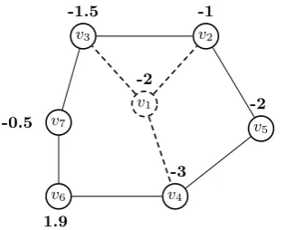
v1

-2

v2

-1

v3

-1.5

v4

-3

v5

-2

v6

1.9

v7

-0.5

Figure 6: Segment of an MWCSP instance. The NPV3test shows that vertexv1and its incident

edges (dashed) can be eliminated.

3.3

Reiteration and Ordering

The settings for the reiteration of the reduction methods within the overall loop as well as for the truncation of the latter are identical to the settings for the PCSTP, see Section 2.4.

Naturally, empirically less expensive tests are performed first. In this way, the DA test, which is both theoretically and empirically the most expensive reduction method, is performed at the end of the loop. Moreover, all other tests are performed prior to the execution of the NPVk test,

in order to reduce the degree of vertices. For the extensive reduction package we execute the advanced CNS test once the reduction loop has terminated and run the entire reduction loop again if eliminations can be performed by the advanced CNS test.

4

Computational Results

This section evaluates the various reduction methods introduced in this paper on several bench-mark test sets for the MWCSP, the PCSTP, and the RPCSTP. To this end, computationally experiments are performed on problems collected for the 11th DIMACS Challenge [1]. In ad-dition, a number of MWCSP instances collected from a computational biology application are considered.

The computational experiments were performed on a cluster of Intel Xeon X5672 CPUs with 3.20 GHz and 48 GB RAM, running Kubuntu 14.04 and using _SCIP 3.2 [16]. For the computations with_SCIP-Jack, CPLEX 12.6.22_{was employed as the underlying LP solver. For}

all computations a time limit of two hours was set.

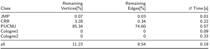
When providing average values we will proceed in two ways: First, for the remaining vertices (edges) of a test set the percentage of remaining vertices (edges) for each instance is computed and the arithmetic mean of these percentages is provided. Second, the solving time of both the reduction package and _SCIP-Jackare computed by taking theshifted geometric mean [2]: Given valuest1, ..., tk∈R≥0, and ashift s∈R≥0, the shifted geometric mean is defined as

k

v u u t

k Y

i=1

(ti+s)−s. (40)

Compared to the arithmetic average, the use of a geometric mean brings the benefit of reducing the influence of very hard instances. On the other hand, the use of a shift is motivated by the endeavor to reduce the effect of very easy instances on the mean value. In the subsequent computations, a shift ofs= 1 is used.

Finally, if an instance has been solved to optimality by the reduction techniques, in the statistics the number of remaining edges and vertices is assumed to be 0.

4.1

(Rooted) Prize-Collecting Steiner Tree Problem

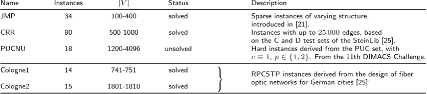
Table 1 provides a brief description of the five benchmark test sets that are used for the com-putational evaluation of the (R)PCSTP reduction techniques. In each line the name of the test set is given in the first column. The next column lists the number of instances within the test set, thereafter the range of the number of vertices for the individual instances within the class is given. Furthermore, the Status indicates whether all instances of a class have been solved in the literature. Conclusively, some elementary characteristics including the origins of the test set are provided.

Name Instances |V| Status Description

JMP 34 100-400 solved Sparse instances of varying structure, introduced in [21].

CRR 80 500-1000 solved Instances with up to25 000edges, based on the C and D test sets of the SteinLib [25]. PUCNU 18 1200-4096 unsolved Hard instances derived from the PUC set, with

c≡1,p∈ {1,2}. From the 11th DIMACS Challenge. Cologne1 14 741-751 solved 

 

RPCSTP instances derived from the design of fiber optic networks for German cities [25].

Cologne2 15 1801-1810 solved

Table 1: Classes of (R)PCSTP instances.