The efficiency of production processes has been the focus of attention of economists since the middle of 20th century. in case of agricultural production,
the evaluation of efficiency is especially complicated not only because of the instability of meteorological conditions, but also due to the large variability of farms with respect to their sizes and production profiles. on the other hand, in the European Union (EU) since the beginning it has been attempted to eliminate the differences between regions, either by supporting the economically weaker regions or by strengthening the specific sectors of economy. in particular, the objec-tive of the common Agricultural Policy in the initial period was to assure food security, and in the course of its further reforms, to increase the professional activity of rural communities, as well as to improve the efficiency of agricultural production.
in 2004, the EU was enlarged to incorporate ten new states. This extension has had an impact on agriculture in the new member states, which were characterized by a high share of this sector of
econ-omy in the generation of gDP and at the same time, a high employment level as well as a considerable diversity of organizational structures. A review and synthesis of several papers analyzing different factors determining the efficiency of agricultural production in the central and Eastern European countries in the 1990’s was presented by gorton and Davidova (2004). Following 2004, agriculture in the new EU member countries faced a new economic situation. Subsidies, new potential sale markets for goods and new possibilities to purchase means of production were found, but at the same time, the pressure of competition increased, leading as a result to the ne-cessity to improve efficiency, and as a consequence to improve profitability.
The main aim of this study is to consider the question whether a higher specialization and a bigger economic size class of farms determine a higher technical ef-ficiency at the same scale for farms from the new and old countries of the EU. This hypothesis is analyzed at the regional level in reference to only two types of
Productivity and efficiency of large and small field crop
farms and mixed farms of the old and new EU regions
Lucyna Błażejczyk-Majka
1, Radosław Kala
2, Krzysztof Maciejewski
31
Adam Mickiewicz University in Poznan, Poznan, Poland
2
Department of Mathematical and Statistical Methods, Poznan University of Life
Sciences, Poznan, Poland
3
Department of Product Ecology, Poznan University of Economics, Poznan,
Poland
Abstract:The main aim of the paper is to consider the question whether a higher specialization and a bigger economic size class of farms determine a higher technical efficiency at the same scale for the farms from the new and old countries of the EU. This study is based on the data contained in the Farm Accounting Data network and covers the first four years following the extension of the European Union in 2004. The adopted units comprised average farms representing 80 re-gions belonging to eleven countries of the EU-15 and four new EU member states. The estimation of technical efficiency was conducted using the data envelopment analysis, separately for each of the two types of farms taking into account their economic size. The main findings indicate that the highest efficiency is achieved by the biggest farms, but those from the regions belonging to the new EU members at the same time had a low efficiency of scale, while those belonging to the coun-tries of the EU-15 were operating at a scale close to the optimal. Moreover, it is confirmed that a longer period of farming under relatively stable conditions promotes a higher efficiency independently of the type of farm production. on the other hand, contrary to the relatively common opinion that a higher specialization promotes a higher efficiency, it was found that field crop farms in average are less efficient than mixed farms, although the difference between efficiencies decreases with an increase of their economic size.
farms, i.e. those specializing in field crops and having multi-directional production. investigations covered the first four years following the enlargement of the EU in 2004. The economic and statistical data were gathered from the Farm Accounting Data network (FADn).
METHODOLOGY
The concepts of efficiency and productivity growth have focused the attention of the economic com-munity since the early papers by Koopmans (1951) and Debreu (1951). in the course of years, several analytical methods have been developed to evaluate technical efficiency. Many details on the early history of the efficiency analysis may be found in an interest-ing study by Førsund and Sarafoglou (2002). These methods represent two fundamentally different ap-proaches. The first one, i.e. the parametric approach, initiated by the studies of Aigner and chu (1968), Timmer (1971) and Afriat (1972), uses the concept of the frontier production function and is based on a respectively modified regression analysis.
The other approach was initiated by Farrell (1957) and it is related with the envelopment of all data points with a non-parametric frontier function. This idea, fully elaborated by charnes et al. (1978), is accomplished by solving a series of linear programming problems, in which the frontiers, i.e. the most efficient farms, are identified by comparing the observed vectors of outputs and inputs characterizing all farms under investigation. This method, known as the data envelopment analysis (DEA), is employed in this investigation. contrary to the parametric approach, it does not require many model assumptions concerning the form of the pro-duction function and the distribution of probability of random components. The only assumptions of the DEA concern the type of technology, which can be constant return to scale (crS) or variable return to scale (VrS), and the type of orientation, which can be focused on outputs maximization given the values of inputs, or on inputs minimization given the values of outputs. Many other formulations of the DEA were reviewed by Thanassoulis et al. (2008) (see also coelli et al. 2005).
in the case of constant return to scale and output oriented DEA, an estimate of technical efficiency is obtained by solving a linear program of the form:
Minθ,λ θ subject: Yλ≥βyi, xi≥Xλ, λ≥0
where xi and yi represent vectors of inputs and out-puts, respectively, of the ith farm, while X and Y are
matrices of input and output vectors of all farms in the sample. The estimated technical efficiency of the ith farm, TE
c(i), is the inverse of optimal value
of β solving the above linear program. When TEc(i) is equal to one, the ith farm is the most efficient in
the whole sample under consideration and will be called a frontier or peer farm. For a more detailed discussion of productivity and efficiency measures, their interpretation and properties, see a monograph edited by Fried et al. (2008).
replacement of the crS technology by the VrS technology results in supplementing the above linear program by an additional condition that all λ’s sum to one. This convexity constraint envelops the data set more tightly, which now is covered by the convex hull rather than the convex cone only, as in the case of the constant return to scale. The corresponding estimate of technical efficiency, TEV(i), called also pure technical efficiency, is not less than TEc(i), and their ratio, SE(i) = TEc(i)/TEV(i), is known as the scale efficiency index. if this index is equal to one, then the farm operates at the optimal scale.
DATA
in this study, we used statistical data published annually by the FADn. The system supplies data with different levels of aggregation focusing on the biggest commercial farms, which jointly in the given region or member state generate at least 90% of the standard gross margin (SgM). The total value of the SgM for each farm makes it possible to determine its economical size, which is expressed in the European size units (ESU). The system distinguishes six classes of farm size, i.e. very small farms (0–4 ESU), small farms (4–8), medium-sized farms (8–16), large farms (16–40), very large farms (40–100) and the biggest farms (over 100 ESU). on the other hand, the share of the individual types of production in the total value of the ESU makes it possible to arrange farms into eight types. As a result, the FADn system dis-tinguishes 24 combinations of types and economic sizes of farms. however, due to the specific agro-technical and climatic conditions, usually only certain types and sizes of farms are found in the individual regions. As a result, in the FADn system, each region is represented by a certain set of average farms, of which each is determined on the basis of a set of farms classified to a specific combination of type and economic size.
the Union in 2004, these regions are divided into two groups, i.e. the old and the new EU countries. Average farms in the individual classes of economic size and representing two economic types, i.e. special-izing in field crops and those with multiple direction production (the mixed type), were assumed as the basic research units in each region. The former of the above mentioned types includes farms where cereals, oil crops and legumes are grown, as well as those with other field and horticultural crops. in contrast, the mixed type comprises farms running simultaneously plant and animal production. Such a selection of units resulted from the decision to possibly confirm or refute the conjecture that mixed farms, considered less economically risky that specialist farms, are at the same time less technically efficient or that it is more difficult to increase their productivity. it is also of some importance that both analyzed types of farms are most popular, particularly in the regions of the new EU member states. in the following part of the paper, the basic units of analysis, i.e. the average farms representing the individual regions, will simply be referred to as farms.
indexes of efficiency were evaluated separately for each of the two types of farms and separately in relation to each year of the analyzed period, us-ing the output-oriented, the sus-ingle-output, and the multi-input DEA. The sum of values of plant and animal production as well as those resulting from the other types of agricultural production activi-ties, except for income from any type of subsidies, were assumed as the output variable. This variable in the FADn nomenclature is referred to as the total output and is denoted as SE131. Production factors (inputs) were assumed to include labour (SE011) ex-pressed in the number of man-hours, i.e. work units (AWU), the total utilized agricultural area (UAA) (SE025), expressed in hectares, the consumption of fixed assets (SE360), referred to as depreciation, expressed by the depreciation deductions in relation to each accounting year as well as working capital, determined as the difference between the total value of inputs (SE270) and the total wages paid (SE370) and depreciation (SE360). The reason why the fixed capital consumption was expressed in values is the fact that the FADn system lacks detailed statistical data on machines and other equipment constituting the components of fixed capital (cf. Larsen 2010). in other studies (see Davidova and Latruffe 2007), the annual consumption of fixed capital apart from depreciation includes also other components, such as e.g. machinery maintenance and fuel costs. in the applied approach, these additional components were incorporated into working capital.
Due to the value-oriented character of variables referring to the volume of production and the values of involved fixed and working capitals, values of these variables were corrected by the price index, i.e. they were expressed in fixed prices from the year 2000, taking into consideration the annual national inflation indexes in relation to the individual inputs. These indexes were taken from the Eurostat report ( http:// epp.eurostat ...). This conversion makes it possible to treat the above mentioned variables as synthetic ag-gregates for the volume of production and the amount of fixed and working capitals, respectively.
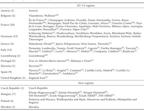
The European Union after its enlargement in 2004 included a total of 122 regions, of which only 96, or 46, respectively, were represented by the average farms classified to at least one of the classes of economic size and specializing in field crops or running mixed-type production. Among these two groups of regions, only 74 and 45 regions, respectively, were represented throughout the entire period of 2004–2007 by the same average farms in terms of economic size. State affiliation of the analyzed regions with the division into the “old Union” (EU-15) and its new members is presented in Table 1.
As it may be easily observed, among the regions mentioned in Table 1, there are regions varying in area. For example Poland is divided into 4 regions, whereas France, being almost two times bigger, is divided into 22 regions. This means that the numbers of farms, on the basis of which average farms were identified, were not uniform. This does not change the fact that averaging, leading to the experimental units assumed in this study, limits the effect of erroneous observa-tions and outliers. Moreover, regions vary in terms of their geographical location, which significantly affects climatic and agronomic conditions. We may mention here regions of Southern Spain or greece and at the same time regions of Belgium or northern germany. As a consequence, we may expect a high variation in values of the analyzed economic indexes. This variation, in view of the above mentioned variables, is reflected in the basic characteristics averaged in relation to years and economic size of the analyzed units, which are presented in Table 2.
better, resulting in a higher productivity of labour and land.
in case of mixed farms, the disproportions between farms from the “old” and “new” regions are much big-ger. The biggest differences were related to the level of fixed and current production factors. in farms from the “old” regions, such a ratio of capital to labour, as well as that of working capital to labour, were six times higher than for the farms from the “new” regions. in view of the above, it is not surprising that the productivity of land in farms from the “old” regions was two times higher and the productivity of labour was even five times higher than in the farms from the “new” regions.
it is also of interest to compare farms in terms of the type of production they run. in the EU-15 regions, productivity of labour and the provision of fixed and working capital for labour in mixed farms was almost two-fold compared to that in field crop farms. in turn, productivity of land and the ratio of working capital to land in mixed farms were higher than in field crop farms by as little as approx. 1/4 and 1/3, respectively. That means that productivity of labour
and land in farms running mixed production were higher than in the farms specializing in field crops at a markedly higher provision of fixed and working capital in the former farms.
in turn, in the mixed farms from the “new” regions, productivity of labour and the provision of fixed and working capital to labour were lower than in the field crop farms by approx. 1/3, but productivity of land and the ratio of working capital to land in the mixed farms were by 1/2 higher than in the field crop farms. This confirms a rather obvious statement that in modern agriculture, high productivity of labour is not possible without an adequate supply of fixed and current production factors.
[image:4.595.64.531.76.435.2]Since the class of the smallest economic units turned out to be represented by very limited numbers of farms both in the case of field crop and mixed farms, in further considerations the class of the smallest farms was included into the class of small farms, thus forming the class of 0–8 ESU. As it turned out, these economically smallest farms are represented, except for one greek region, by Polish regions. in view of the earlier investigations, presented in particular in Table 1. regions represented by field crop and mixed farms
EU-15 regions Austria (1) Austria
Belgium (2) Vlaanderen, Wallonie(M)
France (20)
Île de France(F), champagne-Ardenne, Picardie, haute-normandie, centre,
Basse-normandie(M), Bourgogne, nord-Pas-de-calais, Lorraine, Alsace(F), Franche-comté(M), Pays de la Loire, Bretagne, Poitou-charentes, Aquitaine, Midi-Pyrénées, rhônes-Alpes, Auvergne, Languedoc-roussillon(F), Provence-Alpes-côte(F)
germany (12) Schleswig-holstein
(F), niedersachsen, nordrhein-Westfalen, Essen, rheinland-Pfalz, Baden-Württemberg, Bayern, Brandenburg, Mecklenburg-Vorpommern, Sachsen, Sachsen-Anhalt, Thueringen
greece (3) Makedonia-Thraki(F), ipiros-Peloponissos-nissi loniou, Thessalia(F)
italy (15) MarchePiemonte, Lombardia, Veneto, Friuli-Venezia(F), Umbria(F), Lazio(F), Abruzzo(F), Molise(F), Liguria(M), campania, calabria(F), Emilia-romagna(F), Basilicata(F), Toscana(F)(F), Luxembourg (1) Luxembourg(M)
Portugal (2) Tras-os-Montes/Beira interior(M), ribatejo e oeste(F) Slovenia (1) Slovenia(M)
Spain (9) navarraMancha(F)(F), La rioja, Extremadura(F), Aragón(F), Andalucia(F), cataluna(F) (F), castilla-León, Madrid(F), castilla-La United Kingdom (1) England-East(F)
new regions czech republic (1) czech republic
hungary (7) Közép-MagyarországDél-Dunántúl(F), Észak-Magyarország(F), Közép-Dunántúl(F), Észak-Alföld(F), nyugat-Dunántúl(F), Dél-Alföld(F), (F)
Poland (4) Pomorze and Mazury, Wielkopolska and Sląsk, Mazowsze and Podlasie, Malopolska and Pogórze Slovakia (1) Slovakia
a study by Latruffe et al. (2005) it is not surprising, since small and very small farms in terms of their area predominate in Polish agriculture.
We need to mention here remarks presented in the study by Lund (1983) concerning problems with the identification of a commonly acceptable measure of
[image:5.595.64.533.83.522.2]the farm size and the development of their clear-cut classification. however, between the classification of farm size based on the ESU and their average land area, there is a relatively close interdependence, which is confirmed by the average utilized agricultural areas, given in Table 3, for the field crop and mixed farms Table 2. Basic descriptive statistics of farms
Variables
EU-15 regions new regions
mean deviationstandard min max mean deviationstandard min max
Field crop farms
Total output (€ 1000) 125.19 169.35 4.45 1 142.29 178.32 320.90 6.36 1 715.08
Labour (100 AWU) 42.67 38.73 9.42 289.27 117.88 191.26 5.70 867.48
Land (ha) 96.15 141.25 2.31 924.19 241.14 376.37 6.84 1 482.90
Working capital (€ 1000) 83.75 127.72 2.25 861.32 120.63 225.19 3.06 1 187.63
capital (€ 1000) 17.21 21.87 0.02 155.28 20.11 34.32 0.68 249.84
output/Labour 2.47 1.82 0.24 8.68 1.25 0.58 0.21 2.72
output/Land 1,49 0.96 0.25 12.11 0.72 0.23 0.36 1.59
Land/Labour 2.07 1.69 0.09 7.98 1.99 1.08 0.20 4.49
Working capital/Labour 1.62 1.36 0.07 6.38 0.81 0.42 0.09 1.80
capital/Labour 0.37 0.31 0.00 1.43 0.17 0.10 0.04 0.50
Working capital/Land 0.84 0.43 0.14 2.99 0.42 0.10 0.23 0.85
Mixed farms
Total output (€ 1000) 290.80 445.64 12.61 2 842.40 211.37 461.65 4.26 1 744.87 Labour (100 AWU) 72.45 123.55 17.71 774.24 168.84 350.54 23.81 1 639.37
Land (ha) 167.56 270.21 11.51 1 523.51 206.93 465.58 5.35 1 856.07
Working capital (€ 1000) 209.89 323.83 6.08 2 044.30 142.35 324.02 2.51 1 259.76
capital (€ 1000) 40.13 56.16 0.66 369.95 28.21 79.71 0.83 483.66
output/Labour 4.17 1.93 0.41 8.26 0.83 0.55 0.16 2.00
output/Land 2.02 1.05 0.29 6.78 1.05 0.25 0.65 1.97
Land/Labour 2.41 1.42 0.39 6.63 0.79 0.52 0.18 1.94
Working capital/Labour 3.03 1.45 0.20 5.85 0.50 0.35 0.09 1.25
capital/Labour 0.64 0.37 0.02 1.62 0.11 0.07 0.03 0.41
Working capital/Land 1.40 0.68 0.16 4.45 0.61 0.16 0.38 1.15
Table 3. Average utilized agricultural area of crop and mixed farms Size
(ESU)
Field crop farms Mixed farms
means (ha) standard deviation sample size means (ha) standard deviation sample size
0–8 9.77 19.08 96 8.58 57.99 24
8–16 24.11 15.58 144 19.58 50.22 32
16–40 50.49 13.49 192 32.59 35.51 64
40–100 109.50 12.38 228 82.17 28.99 96
[image:5.595.62.535.650.767.2]in the individual classes of economic size (cf. Lund and Price 1998). in this list, we need to stress the high values of standard deviations, particularly for smaller classes of economic size in mixed farms. however, it does not change the fact that with an increase in the utilized agricultural area of farms, their economic size increases, being the basis for the classification of units in terms of their size applied in this study. As it was expressed by gorton and Davidova (2004) in their review of studies on productivity and efficiency of farms in central and East European countries, this method of determination of size in the analysis of efficiency has been relatively rarely used to date.
MAIN FINDINGS
Technical, pure technical and scale efficiency
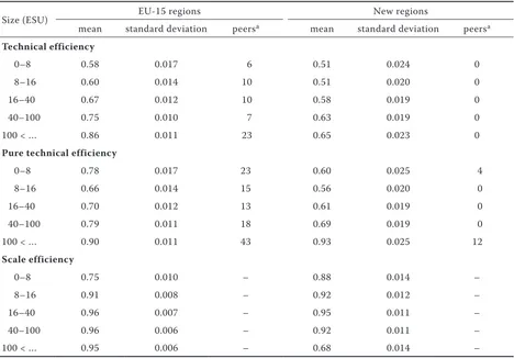
The average values of technical efficiency, TEc, pure technical efficiency, TEV, and scale efficiency, SE, for field crop farms, recorded throughout the entire analyzed period taking into consideration their economic size and the regions of the EU-15 and “new” member states of the EU, are presented in
Table 4. Additionally, standard deviations were given together with the number of peers, showing how many reference units there were, which during at least one year in the analyzed four-year period reached the full 100% technical efficiency or pure technical ef-ficiency. As it may be clearly seen, at the assumption of the crS, the peers are found solely among farms from the “old” EU regions. At the assumption of the VrS, associated with the best practice technology, a vast majority of peer farms was also found in the “old” regions, but such farms appeared also among the economically biggest and smallest farms from the “new” regions.
[image:6.595.65.533.424.750.2]indexes of technical efficiency for the average farms from the “old” regions are markedly higher than those of the farms from the “new” regions, with the differ-ences increasing with an increase in the economic size of farms. A similar relationship was observed for the pure technical efficiency, but this time the differences were the biggest for the smallest farms and decreased with an increase in the economic size of farms. in turn, indexes of the scale efficiency are high in all cases, except for the smallest farms from the “old” regions and the biggest from the “new” regions. As a result, medium-sized, large and very
Table 4. Average efficiency of field crop farms
Size (ESU) EU-15 regions new regions
mean standard deviation peersa mean standard deviation peersa
Technical efficiency
0–8 0.58 0.017 6 0.51 0.024 0
8–16 0.60 0.014 10 0.51 0.020 0
16–40 0.67 0.012 10 0.58 0.019 0
40–100 0.75 0.010 7 0.63 0.019 0
100 < … 0.86 0.011 23 0.65 0.023 0
Pure technical efficiency
0–8 0.78 0.017 23 0.60 0.025 4
8–16 0.66 0.014 15 0.56 0.020 0
16–40 0.70 0.012 13 0.61 0.019 0
40–100 0.79 0.011 18 0.69 0.019 0
100 < … 0.90 0.011 43 0.93 0.025 12
Scale efficiency
0–8 0.75 0.010 – 0.88 0.014 –
8–16 0.91 0.008 – 0.92 0.012 –
16–40 0.96 0.007 – 0.95 0.011 –
40–100 0.96 0.006 – 0.92 0.011 –
100 < … 0.95 0.006 – 0.68 0.014 –
large farms from the “old” and “new” regions are characterized by a relatively low pure technical ef-ficiency and high scale efef-ficiency. it means that in those farms, inefficiency results from the problems connected with an appropriate management or utili-zation of resources. in farms from the “new” regions, these problems are much bigger and may additionally result from the excessive labour force and a lower productivity of labour and land (cf. Buckwell and Davidova 1993). it needs to be stressed here that efficiency and productivity of agricultural activity are to a considerably degree determined also by the factors hardly definable in quantitative studies, i.e. environmental conditions including such factors as soil quality, climate, precipitation, etc. (cf. Benjamin 1995; Bhalla and roy 1988; Davidova et al. 2002). For example, environmental conditions in the regions of northern Spain or central France are obviously more advantageous than e.g. in the regions of Poland or hungary.
From the evaluations contained in Table 4, it fol-lows also that efficiency determined in reference to the best practice for the economically smallest farms (0–8 ESU) is higher than for bigger farms (8–40 ESU) in the regions of the EU-15. Such dependence, although
to a lesser degree, is also found for farms from the “new” EU regions. This observation corresponds with a finding reported in the study by Latruffe et al. (2005), who presented among other things the inves-tigations on the efficiency of crop farms in Poland. however, the direct consistency of these remarks is limited, since in the above mentioned publication, farms represented only Polish agriculture, the size of farms was expressed by the cropped area and the number of size intervals was bigger, and they included first of all smaller farms, which in the classification according to the ESU from Table 3 would be classi-fied to the first three categories. Still the smallest and small farms, typically based on labour of family members, create better conditions for an enhanced control of technology and more economical utiliza-tion of inputs.
[image:7.595.65.534.425.751.2]According to the pure technical and scale effi-ciency indexes from Table 4, the biggest farms from the “new” EU regions are usually very efficient, but they exhibit a low productivity, while the smallest farms are much less efficient and more productive. it needs to be stressed here that the biggest farms in the “new” regions were founded mainly through the transformation of the former state-owned or
Table 5. Average efficiency of mixed farms
Size (ESU) EU-15 regions new regions
mean standard deviation peersa mean standard deviation peersa
Technical efficiency
0–8 – 0.63 0.022 0
8–16 0.76 0.027 1 10 0.66 0.027 0
16–40 0.77 0.016 12 3 0.74 0.024 0
40–100 0.75 0.012 0 –3 0.78 0.027 0
100 < … 0.87 0.011 19 18 0.69 0.031 0
Pure technical efficiency
0–8 – 0.87 0.019 11
8–16 0.90 0.024 4 21 0.69 0.024 0
16–40 0.88 0.014 19 11 0.77 0.021 0
40–100 0.87 0.011 16 5 0.82 0.024 1
100 < … 0.93 0.009 30 –5 0.98 0.027 7
Scale efficiency
0–8 – 0.73 0.019 –
8–16 0.85 0.023 – 0.97 0.023 –
16–40 0.87 0.014 – 0.97 0.020 –
40–100 0.87 0.010 – 0.95 0.023 –
100 < … 0.94 0.009 – 0.71 0.026 –
cooperative farms, which may have problems with the rational utilization of resources. in fact, a more in-depth analysis makes it possible to determine that throughout the entire period of analysis, these farms were operating at a decreasing return to scale (DrS). in turn, the smallest farms were operating at an increasing return to scale (irS). This means that in an attempt to improve productivity in the former case, while maintaining a high efficiency, the scale of farms should be reduced, whereas in the latter case, it should be the opposite, i.e. the scale should be increased. The biggest farms from the EU-15 regions are closest to the optimal scale, being at the same time characterized by both high technical ef-ficiency and high pure technical efef-ficiency, and as a consequence, also a high scale efficiency.
Table 5 presents averages (together with standard deviations) from the four years of the 2004–2007 period for the efficiency of farms running mixed pro-duction. in this case, among the farms representing the EU-15 regions, there were no economically small-est farms. Thus, the potential comparisons pertain only to the other size classes. Similarly as in case of the field crop farms, the numbers of peers under the assumption of the crS are found only in the group of farms representing the “old” regions, with the biggest number of peers being found among the economi-cally biggest farms. Also taking into consideration the best practice technology (VrS), peers are found first of all among the farms from the “old” regions, but among the smallest and biggest farms from the “new” EU regions peers were also recorded.
Values of technical and pure technical efficiency for farms from the EU-15 regions are bigger than for the other group of regions, except for the very big and biggest farms. At the same time, the indexes of pure technical and scale efficiency for farms from the EU-15 regions were relatively high, which in-dicates a relatively efficient technology with only slight corrections in scale. in this group, the eco-nomically biggest farms are exceptional, running technically efficient production at a scale closest to the optimal scale.
in turn, indexes of pure technical efficiency for the medium-sized and large farms from the “new” regions were low, and those of scale efficiency were high, which may indicate that inefficiencies are caused by the inappropriate management or erroneous uti-lization of resources. in the economically biggest farms, the indexes of pure technical and scale effi-ciency were opposite – the former being very high, while the latter – is very low. This means that at the maintenance of high efficiency and at a change in the scale of production, and in fact by its reduction, a
higher productivity could be obtained in those units. in the case of farms from the “new” regions, it also turned out that in relation to the best practice, the economically smaller farms are more efficient than the medium-sized farms. however, the scale efficiency index of the smallest farms is low, which also indicates a potential for an improvement of productivity, but this time by increasing the scale of production.
Slacks
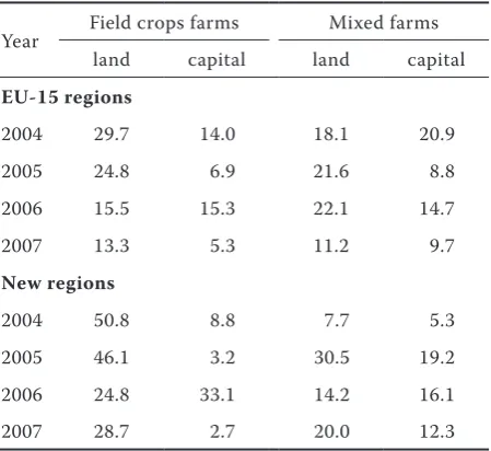
The DEA revealed also excess inputs. Percentage values of slacks for the most excessive inputs are presented in Table 6. in case of the analyzed farms, considerable values of slacks were recorded only for land and capital. For field crop farms represent-ing the “old” regions, the average percentage land consumption in relation to all farm sizes was 23%, which means that at a reduction of the cropped area in average by 23% it would be possible to obtain the same economic results. however, it needs to be re-membered that as a result of a considerable variation of the analyzed regions in terms of their climatic and agricultural conditions, the values determined here need to be considered with caution. As a result, slacks indicate only the directions in which improvements of technology may be searched for.
[image:8.595.307.532.561.767.2]First of all, it needs to be remembered that average excessive land consumption in farms from the “old” regions, specializing in field crops, was here much smaller than in the analogical farms from the “new” regions. Moreover, over the period of four year, the excessive land consumption in farms from the “old” EU regions decreased from approx. 30% in 2004 to
Table 6. input slacks for technical efficiency (in %)
Year Field crops farms Mixed farms
land capital land capital
EU-15 regions
2004 29.7 14.0 18.1 20.9
2005 24.8 6.9 21.6 8.8
2006 15.5 15.3 22.1 14.7
2007 13.3 5.3 11.2 9.7
New regions
2004 50.8 8.8 7.7 5.3
2005 46.1 3.2 30.5 19.2
2006 24.8 33.1 14.2 16.1
13% in 2007, and in the farms from the “new” regions, it decreased from 51% to 29%. This shows a progress-ing rationalization of the land use, connected with its improved productivity.
in mixed farms, the changes related to the excessive land use were not as marked or clear-cut. in farms from the “old” and “new” regions, the average excess land utilization was observed at a similar level and in comparison to the field crop farms, it was markedly lower. however, no definite trend results issued from the presented statistics, which may confirm that at the mixed-type production the risk of the deteriorated utilization of this resource is higher.
in case of fixed capital, the situation is also far from clear. The average values of the excessive capital con-sumption for the field crop farms amounted to 10% in the “old” regions and 12% in the “new” regions, and they were slightly lower than in the case of mixed farms. in the successive years, these indexes changed rather irregularly, which may be related with the volume of production in the individual years. Values determined here may hardly be compared with those recorded by other authors, but e.g. Latruffe et al. (2005) in their investigations conducted in 1996 and 2000 reported that in the Polish field crop farms, the exces-sive capital consumption in both years was around 10%, while that of land – approx. 4%, whereas in the livestock farms, the excessive capital consumption was as high as 21% in 1996 and only 4% in 2000.
CONCLUSIONS
in this study, an analysis was conducted regard-ing the agricultural production of average farms representing the individual regions of the European Union in the years 2004–2007. The analysis was made based on the data available in the FADn system and concerned farms of different economic sizes and two economic types, i.e. those specializing in the field crops and running mixed production. in these investigations, four basic inputs were included, i.e. labour (AWU), utilized agricultural area (UAA) and the consumption of both fixed and working capital. in view of the enlargement of the European Union in 2004, the regions were divided into two groups. one group, the EU-15, comprised the regions, which were parts of the EU before 2004, referred to as the “old” regions, while the other group included the “new” regions, incorporated in the EU in 2004.
The main objective of the analysis was to find an answer to the question whether the efficiency increases with an increase in the economic size of farms inde-pendently of their level of specialization and at the
same rate for the farms from the “new” and “old” EU member states. This question was referred to field crop farms and mixed farms, the latter considered as less economically risky and at the same time less technically efficient than the former ones.
Efficiency was evaluated using the output oriented DEA separately in relation to each year and separately for field crop farms and mixed farms, in both cases for farms of all economic sizes. At the assumption of the crS, the estimates of technical efficiency were produced, while at the assumption of the VrS, the estimates of pure technical efficiency associated with the best practice technology were established.
Field crop farms
The performed analysis leads to a conclusion that in average, for the field crop farms the lowest pure technical efficiency was found for the units classi-fied to intermediate classes of economic size, while the farms from the “old” regions are characterized by the efficiency higher by approx. 10 percentage points than the farms from the “new” regions. The main reason for such a low efficiency may result from an inappropriate management or poor utilization of resources, while in the “new” regions; it was addition-ally related with a lower productivity of labour and the necessity to adapt to the “new” market economy conditions.
The smallest farms were distinguished by a higher efficiency that the economically bigger farms, but in farms from the “new” regions, it was much lower (by 18 percentage points) than in the “old” regions. At the same time, the index of the scale efficiency in farms from the “new” regions was markedly higher than for the farms in the “old” regions. These facts are, on one hand, consistent with the inverse hypoth-esis that smaller farms are more productive (see e.g. Barrett 1996; gorton and Davidova 2004), but on the other hand, they show that a further improvement of efficiency in the farms from the “old” regions is possible first of all through an increase in scale, while maintaining or improving technology, whereas in the farms from the “new” regions, it is first of all through an improvement of technology.
big-gest farms from the “old” regions were closest to the optimal scale, being at the same time distinguished by both a high technical efficiency and a high pure technical efficiency. Thus, the relatively obvious fact is confirmed that a longer period of farming under relatively stable conditions makes it possible to develop better organizational and technological solutions and as a result, it promotes a higher ef-ficiency and productivity. This conclusion finds an indirect confirmation in the land management, which for the field crop farms is a key resource. For farms from the “old” regions, the excessive use of this input was much lower than in the farms from the “new” regions. Moreover, in the analyzed period, the rate of the decrease in the excessive land use in the farms from the “old” regions was bigger than in the farms from the “new” regions.
Mixed farms
results recorded for mixed farms in relation to the pure technical efficiency also indicate a bigger efficien-cy of the farms from the “old” regions in comparison to the farms from the “new” regions, except for the biggest farms. Moreover, the differences decrease with an increase in the economic size. if for smaller farms the difference was approx. 20 percentage points, then for very big farms it was only 5 percentage points. in turn, the indexes of scale efficiency for medium-sized farms from the “new” regions are higher than for the farms of a similar size from the “old” regions. This means that the scale of the former farms was close to optimal, and their inefficiency was caused by an inappropriate management or an inadequate utilization of resources. in turn, in farms from the EU-15 regions, better economic effects of farming may be obtained through the corrections of scale, which should still be accompanied by an improve-ment of technology.
in the case of mixed farms from the “new” regions, it also turned out that the pure technical efficiency in the smallest farms was bigger than in the economi-cally bigger farms, which also seems to confirm the above mentioned inverse hypothesis.
Finally, let us focus on the economically biggest farms. results recorded for this group of farms are almost exactly the same as for the biggest field crop farms. Thus we may repeat here the remark made earlier that a longer farming under stable conditions makes it possible to develop better organizational and technological solutions, resulting in an increase of efficiency, and as we can see, it is not connected with the type of farm production.
Field crop farms vs. mixed farms
A comparison of field crop farms with mixed farms leads to a conclusion that in the “old” regions, the former farms are in average less efficient than the latter, with the differences between efficiencies de-creasing with an increase in the economic size of farms. This conclusion, pertaining to units operating over a long period under stable conditions, does not confirm the relatively common opinion that a higher specialization promotes a higher efficiency. in turn, the indexes of scale efficiency for field crop farms were higher than for mixed farms, which may mean that at the mixed-type production, it is more difficult to determine an appropriate level of inputs.
in the “new” regions, the relationships between effi-ciencies are similar, i.e. the average field crop farms were less efficient than the mixed farms, with the differences between them decreasing with an increase in the farm size. The indexes of scale efficiency for the field crop farms in the case of medium-sized, big and very big farms were high, but lower than for the mixed farms, which mean that the scale of production in the latter was very close to the optimal scale. These indexes mean that mixed farms of these three intermediate economic size classes were better managed than the field crop farms. A justification for this rather unexpected conclu-sion may be found in the fact of a bigger dependence on the agro-meteorological conditions for the results of field crop farms than mixed farms.
Acknowledgments
This paper was supported by the Funds for Sciences 2008–2011 under the grant no. 111 114034.
REFERENCES
Aigner D.J., chu S.F. (1968): on estimating the industry production function. American Economic review, 58: 226–239.
Afriat S. (1972): Efficiency estimation of production func-tion. international Economic review, 13: 568–598. Bhalla S., roy P. (1988): Mis-specification in farm
produc-tivity analysis: role of land quality. oxford Economic Papers, 40: 55–73.
Barrett c.B. (1996): on price risk and the inverse farm size-productivity relationships. Journal of Development Economics, 51: 193–215.
Buckwell A., Davidova S. (1993): Potential implications of land reform in Bulgaria. Food Policy, 18: 493–506. charnes A., cooper W.W., rhodes E. (1978): Measuring the
efficiency of decision making units. European Journal of operational research, 2: 429–444.
coelli T.J., rao D.S.P., o’Donnell c.J., Battese g.E. (2005): An introduction to Efficiency and Productivity Analysis. 2nd ed. Springer Science + Business Media, new York. Davidova S., gorton M., ratinger T., zawalinska K., iraizoz
B., Kovacs B., Mizik T. (2002): An Analysis of competi-tiveness at Farm Level in cEEcs. EU FP5iDArA Project. Working Paper Series. Working paper 2/11, imperial college at Wye, London.
Davidova D., Latruffe L. (2007): relationships between technical efficiency and financial management for czech republic farms. Journal of Agricultural Economics, 58: 269–288.
Debreu g. (1951): The coefficient of resource utilization. Econometrica, 19: 14–22.
Farrell M.J. (1957): The measurement of productive ef-ficiency of production. Journal of the royal Statistical Society, Series A, 120: 253-281.
Fried h., Lovell K., Schmidt S. (2008): Efficiency and pro-ductivity. in: Fried h., Lovell K., Schmidt S. (eds.): The Measurement of Productive Efficiency and Productive growth. oxford University Press, oxford, new York. Førsund F.r., Sarafoglou n. (2002): on the origins of data
envelopment analysis. Journal of Productivity Analysis, 17: 23–40.
gorton M., Davidova S. (2004): Farm productivity and ef-ficiency in the cEE applicant countries: a synthesis of result? Agricultural Economics, 30: 1–16.
Koopmans T.c. (1951): An analysis of production as an efficient combination of activities. in: Koopmans T.c. (eds.): Activity Analysis of Production and Allocation. cowles commission for research in Economics, Mono-graph no. 13. Wiley, new York.
Larsen K. (2010): Effects of machinery-sharing arrange-ments on farm efficiency: evidence from Sweden. Ag-ricultural Economics, 41: 497–506.
Latruffe L., Balcombe K., Davidova S., zawalinska K. (2005): Technical and scale efficiency of crop and livestock farms in Poland: does specialization matter? Agricultural Economics, 32: 281–296.
Lund P. (1983): The use of alternative measure of farm size in analysis of size and efficiency relationships. Journal of Agricultural Economics, 34: 189–197.
Lund P., Price r. (1998): The measurement of average farm size. Journal of Agricultural Economics, 49: 100–110. Thanassoulis E., Portela M., Despić o. (2008): Data
en-velopment analysis: the mathematical programming approach to efficiency analysis. in: Fried h., Lovell K., Schmidt S. (eds.): The Measurement of Productive Efficiency and Productive growth. oxford University Press, oxford, new York.
Timmer P. (1971): Using a probabilistic frontier produc-tion funcproduc-tion to measure technical efficiency. Journal of Political Economy, 79: 776–794.
Eurostat. Available at http://epp.eurostat.ec.europa.eu/ portal/page/portal/eurostat/home
Arrived on 9th March 2011
Contact address: