A fixed count sampling estimator of stem density based on a survival function

JOURNAL OF FOREST SCIENCE, 61, 2015 (11): 485–495

doi: 10.17221/46/2015-JFS

A fixed count sampling estimator of stem density

based on a survival function

S. Magnussen

Natural Resources Canada, Canadian Forest Service, Victoria BC, Canada

ABSTRACT: In fixed count sampling (FCS) a fixed number (k) of observations is made at n randomly selected sam-ple locations. For estimation of stem density, the distance from a random samsam-ple location to the k nearest trees was measured. It is known that practical FCS estimators of stem density are biased. With the objective of reducing bias in FCS estimators of stem density, a new estimator derived from a survival function with distance acting as time was presented. To allow for spatial heterogeneity in stem density, the survival function includes shared frailty. Encouraging results with k = 6 in terms of bias, root mean squared error (RMSE), and coverage of nominal 95% confidence intervals were obtained in an extensive testing with simulated random sampling from 54 actual and four simulated spatial point patterns of tree locations. Sample sizes were 9, 15, and 30, with 1200 replications per setting. The performance across sites of the new FCS estimator was variable but almost paralleled that of a design-based estimator with fixed area plots. Users of the new FCS estimator can expect an absolute relative bias and a root mean squared error that are 1% greater than for sampling with fixed area plots holding an average of k trees. The chance of a smaller RMSE with the proposed estimator was estimated at 0.44.

Keywords: bias; coverage; forest inventory; spatial point pattern; standard error; root mean squared error

In forestry application of fixed count sampling (FCS) a fixed number (k) of trees closest to each of

n randomly selected sample locations is observed and recorded for attributes (Y) of interest (Morisita 1954; Shanks 1954; Persson 1964; Payandeh, Ek 1986). Density estimators derived from FCS are biased because the inclusion area of the k trees depends on the sample location (Moore 1954; Eberhardt 1967; Ohtomo 1971; Pollard 1971; Cox 1976). The bias can be estimated analytically if and only if the spa-tial point pattern is consistent with a realization from Poisson process (Moore 1954; Pollard 1971) or a negative binomial distribution (Eberhardt 1967).

In difficult terrain and in populations with a high and variable local density of elements, the FCS can be faster and more expedient than sampling with fixed area plots (Cox 1976; McNeill et al. 1977; Chen, Tsai 1980; Patil et al. 1982; Roser et al. 1984; Delince 1986; Jianrang 1988; Lessard et al. 1994; Barbour, Gerritsen 1996; Lynch, Rusydi 1999; Doberstein et al. 2000; Lessard et al. 2002; Picard et al. 2005; Kleinn, Vilčko 2006b; Haxtema et al. 2012).

Efforts to address the bias problem in FCS have been considerable, especially in the context of for-est management inventories, and they reflect a general interest in this sampling scheme (Persson 1964; Cox 1976; Kleinn, Vilčko 2006a, b; Mag-nussen et al. 2008a; Kronenfeld 2009; Noth-durft et al. 2010; Magnussen et al. 2011, 2012a, b, 2014). Design-unbiased FCS density estimators are possible (Kleinn, Vilčko 2006a; Fehrmann et al. 2011) but remain impractical.

Kronenfeld 2009) illustrates the complexity and difficulty of reducing the bias problem in general.

Five recently proposed and broadly applicable FCS stem density estimators (Nothdurft et al. 2010; Magnussen et al. 2011; Magnussen 2012a, b; Magnussen 2014) appear to have reduced the bias to a range (–6 to +6%) where it is likely to be of lim-ited practical concern in FCS with k-values of 4, 5, or 6, and a relatively small sample size (n ≤ 50). However, two of the five estimators are of limited practical utility as they incur a non-trivial compu-tational burden (Nothdurft et al. 2010; Mag-nussen 2012b). Although the bias problem was effectively addressed in the remaining three FCS density estimators (Magnussen et al. 2011; Mag-nussen 2012a, 2014), their performance in terms of root mean squared error (RMSE) and coverage rates of nominal 95% confidence intervals (cCI95) still lags behind the performance with a compara-ble fixed-area plot design.

In a quest to further reduce bias and improve RMSE and cCI95 of FCS density estimators, this study proposes a new estimator of stem density derived from a parametric survival function (Hos-mer, Lemeshow 1999) whereby the distance (d_ij) from the ith _{sample location (i = 1, …, n) to the j} nearest tree (j = 1, …, k) serves as ‘survival time’. Estimation of a parametric survival function pro-vides a model for the probability of observing a dis-tance to the 1st_,2nd_{,…., k}th _{nearest tree equal to or} less than some user-specified distance. To compute an expected ‘survival’ distance and subsequently a stem density, one also needs an estimate of the probability distribution function of distances in the sampled population. A complicating factor, howev-er, is the common phenomenon of local variation in stem density (Clayton, Cox 1986; Picard et al. 2005; Kronenfeld 2009; Nothdurft et al. 2010). In the context of FCS, a local variation in stem den-sity becomes apparent when the variance in the distance to the kth _{nearest tree is larger than in a} forest with a Poisson distribution of stem locations (Thompson 1956). If the k-nearest trees are con-sidered as a cluster, a local variation in stem densi-ty will generate a positive intra-cluster correlation among the k distances observed at a single sample location. The local variation in stem density can be captured in a survival function by adding a random ''cluster'' effect called frailty (Wienke 2010). Since the effect is viewed as shared among the k trees, it is called a shared frailty.

The proposed FCS estimator of stem density is tested on a set of 54 actual and four simulated spatial point patterns of forest tree locations. The

same point patterns have been used in previous assessments of novel FCS estimators of stem den-sity (Magnussen et al. 2011, 2012a; Magnussen 2014). A wide variation in the test patterns allows a generalization of the performance assessment be-yond a forest management inventory.

MATERIAL AND METHODS

The proposed FCS estimator of stem density

( )

( )k S

λ _{is designed for simple random sampling} (SRS) of n sample locations in a finite-area popu-lation with a countable finite number of trees. At each of the n sample locations, the distances from the sample location to the k nearest trees are mea-sured. The proposed estimator takes the same form as a maximum likelihood estimator (MLE) of stem density in a Poisson point pattern (Pollard 1971). However, model-dependent predictions are used in place of observed distances. The proposed estima-tor is given in Equation 1:

( )

(

)

( )

2 2

ˆk S

n k _{n k k}

k c k c

E d _{E d V d}

λ

π _π

− −

= =

  _{  +}

  _{ }

 

 _{ } (1)

where:

k – fixed number of trees to include in the sample at a random sample point,

c – model-dependent bias correction term,

n

E – expectation over the sample, ik

d

– model-dependent prediction of the expected distance from a random sample location (i) to the k-nearest element,

( )

k

V d _{– model-dependent prediction of the variance in} distancesdk to the kth nearest tree.

The rationale for using model-dependent predic-tions in Eq. (1) as opposed to the observed distance data rests with an expectation that a modelling of distances by a parametric survival function with a shared frailty will reduce an otherwise expected bias in the MLE estimator for a Poisson forest.

The model-dependent predictions and bias-correc-tion terms in Eq. (1) were obtained by assuming that one minus the cumulative distribution function of distances F_ij (d) from a random sample location i, to the jth _{nearest tree follows a parametric survival} func-tion with a shared frailty term (Gutierrez 2002).

dis-tribution function for distances (F (d) = 1 – exp [–τdφ_{]), and a gamma distribution for the shared} frailty term (α). This choice was based on prom-ising results from simulated sampling in four test patterns (see the section on test sites) and choices available in the streg procedure of the STATA®_-13

software (Stata LP, College Station, Texas) (Guti-errez 2002). With these choices and the assump-tion that the Weibull parameter τ is an exponential function of the distance order (i.e. j) we have (Eq. 2):

F_ij (d*) = Pr (d_ij≤ d*) = (1 – exp [–τ_j (d*)φ_]i_{) (2)}

with τ_j = exp [β₀ + β₁log(j)] and α₁~ Gamma(θ–1_,θ)

where d* _{is a user specified distance. Note how the} random frailty term is specific to a location (i) and therefore shared among the distances to the 1, …, kth tree at this location. The parameters Ψ = {_{φ, β0, β1, θ}}

in Eq. (2) were estimated via the method of maximum likelihood (ML) (Cleves et al. 2004) using all n × k

observed distances d_ij in the likelihood under the as-sumption of conditional independence of distances

d_ij, j = 1, …, k given Ψ and θ. It is important to note that the survival function is fitted to all observed dis-tances. Hence, the expected distance to the kth near-est tree cannot be derived directly from the survival function, it has to be weighted by a probability density function of distances to the kth _{nearest tree.}

Alternative models for τ_j in Eq. (2) with squared and inverse transforms of j within the exponent were also explored but without success. A simpler approach using a hazard function in place of a sur-vivor function in Eq. (2) that was also tried, gave a much more variable performance.

As mentioned above, the estimated distribution function of distances is estimated jointly for all n × k

distances. A model-dependent prediction of the ex-pected distance dk appearing in the estimatorλˆS( )k

(see Eq. 1) must therefore be calibrated to the distri-bution of d_k. For the spatial point patterns used in this study, a gamma distribution with parameters {γ ηk, k

}

provides (consistently) a good fit to the distribution of d_k (Magnussen 2012a). As k increases, the bution approaches that of a standard gamma distri-bution

(

ie.γ →k 1,fork→ ∞

)

. With these choices the expected distance was computed as (Eq. 3):

(

)

(

)

(

)

(

)

max

min max

min

d

d d

d

ˆ _{ˆ ˆ} | | ,

ˆ _{ˆ ˆ}

1 | | ,

k k k k k k

k

k k k k k

d F d g d dd

d

F d g d dd

γ η

γ η

′ =

′ −

∫

∫

Ø

Ø

 (3)

where F'(d_k Ψ) is the probability distribution func-tion of d_k, viz. the derivative of the survival func-tion F. In the integrations, the lower 1% and upper

99% quantiles of the gamma distribution were used as integral limits (d_min, d_max) in an effort to reflect a finite domain of tree sizes. The same integration procedure was used to compute the expected vari-ance of dk, viz. V d

( )

k . Specifically, the variance

was computed as the expected value of

(

dk −dk

)

2

over the distributions of d_k using the same integra-tion limits as in Eq. (3).

The bias correction term c_{in Eq. (4) reflects a}

long-standing recognition of the need, in FCS es-timators of density, to correct the count (k) of ele-ments within the circle with a radius d_k (Moore 1954; Morisita 1954; Persson 1964; Pollard 1971; Patil et al. 1982; Delince 1986). Pollard (1971) derived a bias correction factor of 1/n for the Poisson forest. Moore (1954) suggested a mul-tiplicative bias correction of (k-1)/k. Kleinn and Vilčko (2006b) suggested a bias reduction by us-ing the geometric mean of the distances to the kth and (k–1)th _{tree. However, these corrections are} in-efficient beyond a few select types of point patterns (Kleinn, Vilčko 2006b; Magnussen et al. 2008). Instead, the proposed model-dependent bias cor-rection term c _{is the binomial variance of the}

‘sur-vival’ probability of the predicted distancedk. That

is Equation (4):

(

)

(

)

(

)

Pr( ) 1 Pr( )

ˆ _ˆ

with Pr( ) 1 log 1 exp

ik k ik k

ik k j k

c d d d d

d d _{θ τ} dφ

= ≤ − ≤

≤ = − − −

 



  (4)

The bias correction in (4) is similar to a bias cor-rection of the expectation of a log-transformed vari-able (Baskerville 1972; Snowdon 1991). The ran-dom location effect (α_i) acts akin to a cluster effect (Banerjee et al. 2003). If the local density varies at random across a surveyed population, distances to the 1st_{, …, k}th _{element at a single sample location will} be less variable than if the k ordered distances came from k randomly selected locations. Both clustered and over-dispersed point patterns are likely to ex-hibit significant location effects (θ > 1). Converse-ly, a quasi-regular point pattern would exhibit less variation than in a random point pattern (θ < 1). As θ increases, the variance in distances to the jth near-est element also increases, and the distribution of d_ij

becomes increasingly right-skewed. During the computations of ( )k

S

λ

for the four sim-ulated spatial test patterns (see the section on test sites) it became clear that very small and very large estimates of θ led to extreme and implausible esti-mates of point density. It was therefore decided to trim ^θ to the interval [0.01, 6.0]. Less than 1.5% of 208, 800 computed density estimates were affected by the trimming.

Ψ

Ψ

A variance estimator for ( )k S

λ

was derived via the del-ta technique (Kotz, Johnson 1988; Oehlert 1992) applied to the estimator in Eq. (1) with 2

( )

k k

d +V d replaced by the expectation

( )

2

k

E d _{computed over} the gamma distribution g d

(

k| ,γ ηˆ ˆk k

)

. With the

delta technique the variance of ( )k S

λ

is estimated as

( )

(

_{( ) 2}

)

2

( )

₂

variance k

S E dk E dk

λ  

∂ ∂  × _  _{. Although good} results were obtained with this estimator – in terms of matching the empirical variance and coverage of 95% confidence intervals – it did fail on six sites with a relatively low stem density and a visible clustering of tree locations. The reason for the failure was the exponential increase in higher moments in a right-skewed distribution of distances. Instead, we modi-fied the variance estimator obtained from the delta technique and propose the following more robust and conservative estimator of variance

( )

( )

(

(

( )

)

2

)

( )

2 6

4 ˆ

1

k k

S

k

k c V d V

k E d λ

π

− =

−

  

 (5)

The term

( )

6

k

E d in Eq. (5) was computed using the same integration employed for computing an expectation in (3).

The computations behind

λ

S( )k and V

( )

λˆS( )k may

seem daunting; yet attempts at simplifications (e.g. dropping the gamma distribution of distances, or dispensing with the random location effects) led to a significant drop in performance (bias, RMSE, and cCI95). For a single sample with n = 15, the time required to estimate the MLE of ^Ψ, and the gamma distribution parameters with the software pack-age STATA®_{-13 (Cleves et al. 2004) and a typical}

desktop computer is 30–50 s. Generally, computing times were proportional to the estimate of θ.

Assessment of performance. The performance of the proposed FCS estimator in Eq. (1) was as-sessed in simulated random sampling in 58 spatial point patterns (viz. sites). Performance criteria were: bias; root mean squared error (RMSE); how well the replication average of the analytical esti-mator of variance in Eq. (5) tracks (across patterns) the corresponding empirical variance in replicated estimates of density; and the achieved coverage of nominal 95% confidence intervals (cCI95) for the true point density. Bias, for a given test pattern and sample size n, was estimated as the difference be-tween the mean of 1,200 estimates of density

( )

λˆS

and the known densityλsite. Estimates of bias are

given in percent of λsitein order to facilitate

parisons across sites (patterns). A RMSE was com-puted as √(1,200 – 1)–11 1200

(

)

2

, 1 ˆ

(1200 1) rep λS rep λsite

− =

− ∑ − . To facilitate

an among-site comparison, the relative root mean squared error (RRMSE) – computed as RMSE

di-vided by

λ

_site– is reported. Linear regression analy-sis was employed to assess how well the mean of replicated analytical estimates of variance obtained from (5) tracked the corresponding empirical esti-mate of variance across the 58 test patterns (sites). The achieved coverage rate of a nominal 95% con-fidence interval was computed as the proportion of computed normal theory confidence intervals (Ca-sella, Berger 2002) which included

λ

site.

Results obtained with

λ

ˆS were compared to results

with a design-unbiased fixed-area density estimator

FIX

λ

as well as to results with two FCS estimators of density previously proposed by the author. The fixed-area plots used with

λ

FIXwere circular with a

radius r_k that, on a given test pattern (site), included an average of k elements. Hence the expected den-sity is 1 2

k

k r

π

− − _{. Because}

FIX

λ

is only nearly asymp-totically

(

n

→ ∞

)

unbiased (Gregoire, Valentine 2008; Mandallaz 2008), we computed estimates of bias and RMSE as done for

λ

ˆS. This ensures a fair

comparison, since our sampling protocol and num-ber of replications (1,200) did not attest a zero bias in

λ

ˆFIX. The two alternative FCS estimators used in

the comparison are called

λ

ˆV1,

λ

ˆV2 where the sub-script V stands for ''virtual fixed area plot'' (Mag-nussen 2012a); the estimator

λ

ˆV2was intended as a robust version of

λ

ˆV1(Magnussen 2014). Based on results from an intensive testing of both

λ

ˆV1 and

λ

ˆV2 it does not seem presumptuous to con-sider them as two well performing – in terms of bias and RMSE – FCS estimators of density. Al-though the FCS reconstruction density estimator

RDE

λ

by Nothdurft et al. (2010) is asymptotically unbiased, and therefore a natural choice as the cur-rently best FCS estimator of density; computation-al complexities deter use in practice and especicomputation-ally for this study with a large number of Monte Carlo simulations of simple random sampling. In terms of RMSE the estimator

λ

ˆ

V2holds an edge over

λ

RDE

(Magnussen 2014). Computational complexities equally excluded an otherwise attractive FCS esti-mator with evidence-based (Akaike’s Information Criterion) averaging of maximum-likelihood based estimators of density based on 16 different models for the spatial distribution of distances to the kth nearest element (Magnussen 2012b).

The

λ

ˆV1estimator computes density on the basis of a virtual fixed area circular plot with a radius

r_v to be computed from the observed distances. A generic recursive algorithm is used to predict the distance to the k+m nearest element from distances to the k+m–1 and k+m–2 nearest elements (k > 2,

dis-tance to the kth _{element less than r}

v is obtained with a minimum of computational effort (Magnussen 2012a). In

λ

ˆ

V2predictions of distances to the (k+1)th, (k+2)th_{, …, (k+m)}th _{nearest element are based on} a nonlinear model of distance ratios 1

1

k m k m

d

d

−

+

×

+ −

(k > 2, m = 1, …, M) derived from a mixture of ob-served distances and distances predicted with the recursive algorithm used in

λ

ˆ

V1. The use of actual

and predicted distances to fit the nonlinear (Pare-to-type) model of distance ratios was assumed to bestow ‘robustness’ to

λ

ˆ

V2. The performance profile of

λ

ˆ

V1 and

λ

ˆ

V2– across the same 58 spatial point patterns used in this study – was, from a practical perspective, however, quite similar.

Simulated fixed count sampling. Fixed count sampling from a finite area of spatial point locations was simulated with a simple random sampling with-out replacement (SRS) of n out of N possible loca-tions on a regular 1 m × 1 m grid suspended over the area of interest. At each sample location, the distance (d in m) to the nearest k points (elements) is mea-sured. From a sample of n k× distances the density

ˆ

_S

λ

(elements·m–2_{) was estimated as per (1)} subse-quent to a MLE of the parameters ^Ψ in the survival function, and the two parameters

(

γ η

ˆ ˆ_k, _k

)

for the as-sumed gamma distribution of distances. A model-de-pendent estimate of variance in λˆS was obtained via

Eq. (5), and a normal-theory 95% confidence interval was computed by standard techniques (Casella, Berger 2002). The process of sampling and estima-tion was repeated 1,200 times for each sample design and test site (1, …, 58).

Sampling designs were limited to sample sizes

n = 9, 15, and 30. The value of k was fixed at 6. Studies with spatial point patterns of tree locations (Lynch, Rusydi 1999; Lessard et al. 2002; Lynch,

Wittwer 2003; Kleinn, Vilčko 2006b; Magnus-sen 2012b) confirm that FCS designs with k < 6 and

n < 9 frequently generate unacceptable levels of bias (>10%) and unattractive estimates of errors.

To mitigate edge effects in sampling from a finite area (Gregoire, Valentine 2008), a selected sam-ple location within a distance of r_k from the border of a test site was replaced by a randomly selected location from the available N – n choices (Mag-nussen et al. 2011). This ensures a fixed sample size of n. In practice edge effects are mitigated by the ‘mirage boundary’ technique (Lynch 2012).

Test point patterns. Testing of

λ

Swas done with

simulated random sampling from 54 actual and four simulated point patterns. The four simulated point patterns (''random, Matérn, quasi-regular, and Strauss'') served the model development. The remain-ing 54 represent locations of trees (elements) in for-est sites (stands). Point densities in the tfor-est set varied from 0.0046 to 0.7361 elements·m–2_{, and the patterns} ranged from quasi-regular (plantations) over random (Poisson) to strongly clustered. A total of 35 patterns were not statistically different from complete spatial randomness (csr, Illian et al. 2008), and 23 indicated a significant departure from csr (Kolmogorov-Smirnov test applied to the distribution of the distances to the

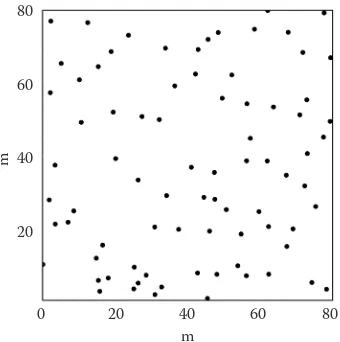
k nearest element, Conover 1980). Further details are provided in (Magnussen 2012b). Nine contrast-ing point patterns have been displayed in Magnus-sen et al. (2011). Six additional patterns were dis-played in (Nothdurft et al. 2010). Additional four of the 24 non-random patterns can be found in Mag-nussen (2014 ). Here the four patterns that gave rise to the largest absolute bias with

λ

ˆ

Sin sampling with

n = 15 are shown in Figs 1 to 4. It is immediately ap-parent why sample-based density estimation is a

[image:5.595.110.239.54.246.2]

chal-Fig. 1. Stem locations in a 6.4 ha old spruce stand in Stand 17 (Schöpfer 1967), stem density 370 ha (site 28)

Fig. 2. Stem map of oak in a stand with a mixture of oak and beech (Manderscheid-198, Rheinland-Pfalz (Ger.),

Pommerening 2002), stem density 125 ha(site 15)

Stand 17

0 20 40 60 80

m 80

60

40

20

[image:5.595.330.500.534.705.2]

lenge in these examples. A test of first-order station-arity in density (Zhang, Zhou 2014) was rejected (P < 0.05) in each of the four examples.

RESULTS

We report results from all 58 point patterns sites without a distinction between the four simulated pat-terns used for model building and the 54 actual test patterns. There was no evidence to suggest a material difference between results from the two groups. Sam-pling with n = 15 is in focus, whereas results for n = 9, and n = 30 are summarily related to the former.

Bias

Over all test patterns and n = 15, the average esti-mate of bias in λˆS was –1.0%. Sampling with fixed

area plots achieved, as expected, the lowest

esti-mate of average bias (–0.5%). Comparable results for

λ

ˆV1and

λ

ˆV2were estimated at –1.0 and 0.4%. As seen in Fig. 5, the range in site-specific estimates of bias is wide for all four density estimators. To wit: a range from –17 to 11% in

λ

ˆFIX; from –12 to 12% in

ˆ

S

λ

; from –18 to 9% in

λ

ˆ

V1; and from –14 to 15% in 2

ˆ

_V

λ

. Centred intervals including 52 of the 58 point patterns (90%) were approximately 25% shorter. In terms of site-specific estimates of absolute bias,

λ

ˆFIX

was again the best (mean 3.3%) followed by nearly equal estimates (3.9–4.1%) for

λ

ˆ

S,

λ

ˆV1 and

λ

ˆV2. Den-sity estimates with

λ

ˆ

FIXwere the least biased in

23 cases but also the most biased in 7 cases. Cor-responding figures were 6 and 17 for

λ

ˆ

S, 13 and 13

for

λ

ˆV1 and 16 and 21 for

λ

ˆV2. Estimates of absolute bias were strongly correlated among the four es-timators (0.92 ≤ _ρ ≤ 0.95_{) indicating a great deal}

of parallelism in relative performance. The strong correlation is also indicated in Fig. 5, where the four estimator-specific scatter in site estimates of bias displays a considerable degree of resemblance. The four patterns with the highest levels of esti-mated bias with

λ

ˆ

S (Figs 1–4) were also included in

the five patterns with the highest estimate of bias in

ˆ

_FIX

λ

,

λ

ˆ ,V1 and

λ

ˆ

V2.

Estimates of bias in sampling with n = 30 were vir-tually identical to those for n = 15. Differences were less than ± 0.3% and within the range of Monte-Carlo errors. Sampling with n = 9, however, resulted in a mi-nor (2.4%) increase in the average estimate of absolute bias in the three FCS density estimators, and a slight (1%) increase in the range of estimates of relative bias in

λ

ˆ

FIX. No other result of practical relevance

emerged from lowering the sample size from 15 to 9. The estimates of bias in

λ

ˆ ,FIX,

λ

ˆ ,V1 and

λ

ˆV2are high-er than those previously reported by Magnussen (2012a, 2014). Previous studies considered the aver-age replicate value of

λ

ˆFIX as the actual true density

(bias = 0). In this study we recognize that in pat-terns with a spatially varying density, the required number of replications needed to ascertain that the bias in

λ

ˆ

FIXis zero, would be impractically large

(> 8,000). A practically relevant comparison of per-formance should therefore recognize, as done here, that the estimated bias in

λ

ˆ

FIXin simulated

sam-pling with a relative small number of replications may not be zero.

Root mean squared errors

The performance with respect to RMSE and

n = 15 indicated a consistent ranking of the four es-timators across the 58 patterns (Spearman rank

[image:6.595.82.271.60.187.2]

cor-Fig. 4. Stem locations of maple in a natural stand of maple and hickory in East Lansing, MI, USA (Hatch et al. 1975), stem density 514 ha (site 11)

Fig. 3. Stem locations in a 3.1 ha stand with beech and shade tolerant hardwoods in Germany in stand 84(Schöpfer 1967), stem density 441 ha (site 51)

Stand 84

0 20 40 60 80 100 m

100

80

60

40

20

[image:6.595.85.266.526.706.2]

relations of 0.97–0.98). This is also apparent in Fig. 5, where the four estimator specific-scatter plots show a great degree of resemblance. The overall average estimate of relative RMSE was 13% for

λ

ˆ ,

FIX14% for

ˆ

_S

λ

and

λ

ˆ

V1 and 16% for

λ

ˆ

V2. In 54 patterns the low-est RMSE was obtained with

λ

ˆ ,FIX and the largest

was obtained with

λ

ˆ

V2. In 39 cases

λ

ˆ

S ranked the

second and

λ

ˆ

V1 _{the third; in 15 cases their}

rank-ing was reversed. As for bias, the site-specific es-timates of relative RMSE varied considerably; from 5 to 33% with

λ

ˆ .

FIX. Wider and right-shifted ranges

were obtained with

λ

ˆ

S (5–40%),

λ

ˆ

V1 (6–37%), and 2

ˆ

_V

λ

(8–42%). The interquartile range of site-specific estimates of relative RMSE was 4% for

λ

ˆ

FIX and 5%

for the FCS estimators.

With the exception of

λ

ˆ

V1 _{increasing the sample} size from 15 to 30 achieved approximately (±2%) the expected (average) reduction in RMSE of (1–2–0.5_{) × 100% ≅ 29% for an unbiased estimator.} The reduction for

λ

ˆ

V1was only 21%. The reduction in RMSE was equally reflected in the range of esti-mates. Results in terms of rankings were not mate-rially affected by the increase in sample size.

Lowering the sample size from 15 to 9 increased, as expected, the RMSE: least (15%) in

λ

ˆ

FIX, and most

(30%) in the FCS estimators. The larger increase in FCS estimators reflects a combination of a small in-crease in bias and a poorer model fit. Apart from the increase in RMSE, all trends across sites and ranking of estimators were very similar to results with n = 15.

The relative frequency with which an estimate of RMSE for

ˆ

λ

ˆ

S was less than the RMSE estimated for

FIX

λ

was 0.44 in this study. Corresponding results for

λ

ˆ

V1 and

λ

ˆ

V2 were 0.43 and 0.42.

Empirical and analytical estimates of variance

A linear regression, with the empirical vari-ance in 1,200 replications of

λ

ˆ

Sas the dependent

variable (n = 15), and the average analytical site-specific estimate of variance as the explanatory variable, achieved an adjusted R-squared value of 0.91, a slope of 1.01 (± 0.04), and a non-significant (P = 0.53) intercept of 0.00. Comparable results for

ˆ

FIX

λ

were: a slope of 0.97 (± 0.004); a non-signif-icant (P = 0.83) intercept of 0.00; and an adjusted R-squared value of 0.99. Regression models for

λ

ˆV1 and

λ

ˆ

V2 had estimated slopes of 1.18 (± 0.01) and 1.19 (± 0.03), both significantly (P < 0.002) greater than 1.0. A graphical display of these results is in Fig. 6. [image:7.595.64.294.54.307.2]

The above regression results were virtually re-peated with n = 30. However, with n = 9 the aver-age of the analytical variance tracked the observed variance less well than with n = 15. The explained

Fig. 5. Bubblechart summaries of estimates of BIAS, RMSE, and cCI95 with λˆFIX(a), λˆS(b), λˆV1(c) and λˆV2(d)

es-timates (grey-tone area of a pie chart indicates cCI95 with the black sliver indicating 1-cCI95, overall (sites) means of the estimates of BIAS and RMSE are indicated by a black dot, horizontal and vertical lines cover an interval from the 0.05 to the 0.95 quantile of the site-specific estimates of BIAS and RMSE)

Fig. 6. Observed variance ofλˆ viz. viz. VVreprep(

( )

λλˆˆ) plotted against viz. Vrep

( )

λˆ

the expected value of the analytical estimator of variance (E_rep[^V

( )

(

(

E Vˆ λˆ 

)

 )]), dashed one-to-one line is added as a visual aide

–20 –15 –10 –5 0 5 10 ^

Bias (%)

–15 –10 –5 0 5 10 15 ^

Bias (%)

1 ˆ_V

λ λˆV₂

35 25 15 5 RM SE (%)^ 35 25 15 5 RM SE (%)^

–10 –5 0 5 10 ^

Bias (%) –15 –10 –5 0 5 10Bias (%)^ ˆ_FIX

λ λˆS

35 25 15 5 35 25 15 5

(a) (b)

(c) (d)

E_rep[^V

( )

(

(

E_repVˆ λˆ 

)

 V1)]

(

ErepErep_V[^ˆV

( )

(λˆV2_)]

)

Vrep

[^ V (

(

)

(

)

ˆ ˆ re p EV λ   V1 )]

Vrep

[^ V (

(

)

(

)

ˆ ˆ re p EV λ   V2 )]

E_rep[^V

( )

(

(

_Erep_Vˆ λˆ 

)

 FIX)]

(

ErepErep_V[^Vˆ

( )

(λˆS)]_

)

Vrep

[^ V (

(

)

(

)

ˆ ˆ re p EV λ   FIX )]

Vrep

[^ V (

(

)

(

)

ˆ ˆ re p EV λ   S )]

(a) (b)

[image:7.595.304.533.467.705.2]

variance dropped by approximately 3%, and es-timates of slopes were either slightly (4%) lower (

(

λ λ

ˆ ˆ_{S, FIX) or slightly (5%) higher (}

)

(

λ λ

ˆ ˆ_{V1, V2). As for}

)

n =15 and n = 30, no intercept was significantly dif-ferent from zero.

Achieved coverage rate of 95% confidence intervals

Normal theory 95% confidence intervals computed on the basis of

λ

ˆ

S and

V

ˆ

( )

λ

ˆ

S achieved an average

cov-erage of 0.93 (site range: 0.46–1.00). With fixed area sampling the average coverage matched the intended coverage to within 0.03% but site-specific results var-ied from 0.57 to 1.00. Computed CI95s from sam-pling with virtual fixed area plots were in most cases too short with an average coverage less than intended (88% forλˆV1, and 90% for

λ

ˆV2). Again, these averages cover a wide range (0.54–0.96) of site-specific results.

Increasing the sample size from 15 to 30 increased the average coverage of CI95s in all four density es-timators by approximately 2%. More importantly the minimum site-specific coverage improved by 12%. When dropping the sample size from 15 to 9, the achieved coverage decreased by approximately 4% in all four density estimators. Otherwise trends and rankings across sites with n = 30 or n = 9 were similar to those with n =15.

DISCUSSION

To consider a distance from a randomly selected point to the jth _{nearest trees as a survival time may} have intuitive appeal but does not, in and by itself,

offer any advantages in the current context of con-structing an FCS estimator of stem density. The key to the relative success of the new proposed estimator rests with the joint estimation of the distribution of the j = 1, …, k distances as a function of log(j) and in-clusion of a random location effect (in density) called a shared frailty. A random location effect cannot be estimated from just the distances to the kth _nearest tree. Replications are needed, and here they are in the form of all k distances. There are two disadvan-tages: (i) the location effect is estimated for an en-semble of ordered distances and not specifically for the distance to the kth _{nearest tree; and (ii) the} esti-mated parametric distribution function of distances is conditional on the order (j) of the distance, hence estimates of means and variances require a calibra-tion to the distribucalibra-tion of the kth nearest trees.

Adopting a survival function modelling frame-work for an FCS estimator of stem density offers an analyst a wide spectrum of flexible survival functions and options to exploit auxiliary vari-ables (Gutierrez 2002; Li, Ryan 2002, 2004; Ba-nerjee et al. 2003; Wienke 2010). It is known that distinct spatial processes generate distinct dis-tributions of distances to the nearest lth _element (l = 1, …, k) (Illian et al. 2008; Oedekoven et al. 2014). For a first-order stationary spatial process generating a point pattern, the ensuing point den-sity is closely linked to the distribution of distanc-es from a randomly selected location to its k near-est neighbours. Identifying the link is a complex challenge, unless the point process is compatible with complete spatial randomness (Thompson 1956; Isham 2010). In this study, a functional link between the four parameters in the survival func-tion, and the point density of a site was not appar-ent. Therefore the benefit of a survival function was limited to the estimation of the parameter in the assumed gamma distribution of the shared frailty viz. heterogeneity in local point density. A benefit that made the performance of

λ

ˆ

S run

al-most parallel to that of

λ

ˆFIX. A consistent relative [image:8.595.68.293.538.690.2]

performance against a benchmark is important from a practical perspective. It allows an analyst a better informed decision when pros and cons of fixed area versus fixed count sampling are consid-ered. A widely fluctuating performance of simpler FSC estimators (Moore 1954; Morisita 1954, 1957; Persson 1964; Eberhardt 1967; Pollard 1971; Cox 1976; Delince 1986; Kleinn, Vilčko 2006b) is an important deterrent except in a few cases when an analyst knows what to expect from a chosen FSC estimator (Lynch, Rusydi 1999; Kleinn et al. 2009).

Fig. 7. Within-site distribution of the estimated variance ^θ

in shared random effect frailty. The sites are listed in order (1 to 58) of processing. The first four are simulated point patterns used for the model development

0 2 4 6 8 10 ^

θ 56

52 48 44 40 36 32 28 24 20 16 12 8 4

Sit

The use of a survival function in an FCS estima-tor of stem density may offer some additional tan-gible advantages, including but not limited to: use of density-dependent explanatory variables (Niel-son et al. 2004); ease of handling censored distanc-es along borders of a finite area population (Lynch 2012); including conditional probabilities of obser-vation (Barbour, Gerritsen 1996; Doberstein et al. 2000; Farnsworth et al. 2002).

The variance of the random and shared frailty ef-fects (θ) was statistically significant in all individual estimates, suggesting either a significant over-dis-persion in local point density (θ < 1) or a significant under-dispersion (θ > 1) relative to that of the com-plete random point pattern. As expected, ^θ was re-lated to the among-plot variance of

λ

ˆFIX. For the 58

sites, a second-degree polynomial with λˆ ( )FIX site as

the dependent and log(–θ^(site)) as the explanatory variable achieved an R-squared value of 0.97 with all polynomial terms highly significantly different from 0 (tˆ≥ 15.7, P < 0.00). Larger values of –θ ^(site) were indicative of a larger within-site variation in local point density. Fig. 7 illustrates, for each site, the distribution of estimated values of θ. Sites with a quasi-regular point pattern are characterized by low values of θ _{with a mean in the interval [0.25;} 0.5] and an interquartile range of approximately 0.2. Strongly clustered sites (e.g. 2, 8, 11, and 17) display not only a large average value of θ, but equally a large among-sample variation in esti-mates of θ. Presumably θ is also related to Ripley’s

K-function (Illian et al. 2008) and could therefore serve as quantitative indicator of the variance in lo-cal density.

Using a survival function facilitated the construc-tion of a bias-correcconstruc-tion term (

( )

c



_{) intended to} coun-teract the effect of using the predicted area of the smallest circle including, on average, the k nearest elements at a randomly chosen sample location (Pollard 1971; Cox 1976; Delince 1986; Picard et al. 2005; Kleinn, Vilčko 2006b). A risk-based approach to constructing a bias-correction term was adopted (Casella, Berger 2002): The risk of using the expected distance as the radius in an as-sumed fixed area circular plot for the calculation of an FCS density estimator was equated to the likelihood that the distance is less than expected, times the likelihood that it is greater. Attempts to replace this risk-based correction term with the more familiar 0.5 (Kleinn 1996) only resulted in an increase in estimates of bias.

From a modelling perspective, this study suggests that improvements in FCS estimators must come from not only in modelling the distribution of

dis-tances but also the within-site variance in local den-sity. A direct modelling of the latter in the form of a marginal distribution of density has met with mixed results (Magnussen et al. 2008b; Magnussen 2012b). Estimating the distribution of frailty appears more promising. A side-effect of estimating a model for frailty and a model for distances is the increase in the number of parameters to be estimated. This puts upward pressure on the required minimum sample size for obtaining results with an acceptable preci-sion. Results from this study suggest a minimum sample size of 12 for the proposed estimator.

The proposed FCS estimator of density appears to hold a small but important advantage over existing practical FCS alternatives, at least in terms of RMSE and cCI95, which are important to both an analyst as well as to users of FCS results. While the marginal advantages across 58 point patterns may seem slim, the correlation among results with

λ

ˆ

FIX and

λ

ˆ

S was

considerably stronger than with the alternatives. The reported performance of

λ

ˆ

Shas been

quanti-fied in terms of averages across sites. However, a strong correlation among site-specific results with

ˆ_FIX

λ _and

λ

ˆ

_Ssupports the expectation of stability in relative performance. Nevertheless, the wide range in performances of the four estimators across sites is an area of concern. The poor performance of all four estimators on a handful of sites – with either a large amount of within-site variation in local point density or a patchy mosaic of areas with distinct differences in point density – reflects that a precise and an accurate estimate of density from such sites is only possible with large samples (e.g. n > 100).

The large variation in the 58 spatial point patterns used in this study vouches for a robust assessment of the proposed FCS estimator of density and allows a generalization of the results to practice, not only in forestry, but also to surveys in biology and ecology where FCS can be attractive (Doberstein et al. 2000; Picard et al. 2005; Steinke, Hennenberg 2006; White et al. 2008).

References

Banerjee S., Wall M.M., Carlin B.P. (2003): Frailty modeling for spatially correlated survival data, with application to infant mortality in Minnesota. Biostatistics, 4: 123–142. Barbour M.T., Gerritsen J. (1996): Subsampling of benthic

samples: a defense of the fixed-count method. Journal of the North American Benthological Society, 15: 386–391. Baskerville G.L. (1972): Use of logarithmic regression in the

Casella G., Berger R.L. (2002): Statistical Inference. 2nd _Ed. Pacific Grove, Duxbury Press: 660.

Chen M.Y., Tsai J.L. (1980): Plotless sampling methods for investigating the arboreal stratum of vegetation. Quarterly Journal of Chinese Forestry, 13: 29–38.

Clayton G., Cox T.F. (1986): Some robust density estimators for spatial point processes. Biometrics, 42: 753–767. Cleves M.A., Gould W.W., Gutierrez R.G. (2004): An

Intro-duction to Survival Analysis Using STATA. College Station, STATA Press: 308.

Conover W.J. (1980): Practical Nonparametric Statistics. New York, Wiley: 592.

Cox T.F. (1976): The robust estimation of the density of a forest stand using a new conditioned distance method. Biometrika, 63: 493–499.

Delince J. (1986): Robust density estimation through distance measurements. Ecology, 67: 1576–1581.

Doberstein C.P., Karr J.R., Conquest L.L. (2000): The effect of fixed-count subsampling on macroinvertebrate biomonitor-ing in small streams. Freshwater Biology, 44: 355–371. Eberhardt L.L. (1967): Some developments in 'distance

sam-pling'. Biometrics, 27: 207–216.

Farnsworth G.L., Pollock K.H., Nichols J.D., Simons T.R., Hines J.E., Sauer J.R., Brawn J. (2002): A removal model for estimat-ing detection probabilities from point-count surveys. The Auk, 119: 414–425.

Fehrmann L., Gregoire T., Kleinn C. (2011): Triangulation based inclusion probabilities: a design-unbiased sampling approach. Environmental and Ecological Statistics, 19: 107–123. Gregoire T.G., Valentine H.T. (2008): Sampling Strategies for

Natural Resources and the Environment. Boca Raton, Chap-man & Hall/CRC: 465.

Gutierrez R.G. (2002): Parametric frailty and shared frailty survival models. The Stata Journal, 2: 22–44.

Hatch C.R., Gerrard D.J., Tappeiner J.C. II (1975): Exposed crown surface area: A mathematical index of individual tree growth potential. Canadian Journal of Forest Research, 5: 224–228.

Haxtema Z., Temesgen H., Marquardt T. (2012): Evaluation of n-tree distance sampling for inventory of Headwater Ripar-ian Forests of Western Oregon. Western Journal of Applied Forestry, 27: 109–117.

Hosmer D.W.Jr., Lemeshow S. (1999): Applied Survival Analysis. Regression Modeling of Time to Event Data. New York, John Wiley & Sons: 386.

Illian J., Penttinen A., Stoyan H., Stoyan D. (2008): Statistical Analysis and Modelling of Spatial Point Patterns. Chichester, Wiley: 534.

Isham V. (2010): Spatial point process models. In: Gelfand A.E., Diggle P.J., Fuentes M., Guttorp P. (eds): Handbook of Spatial Statistics. Boca Raton, CRC Press /Taylor&Francis: 283–298. Jianrang W. (1988): Application of plotless sampling method

to the warm-temperate deciduous broad-leaved forests. Acta Botanica Boreali-occidentalia Sinica, 1: 7.

Kleinn C. (1996): Ein Vergleich der Effizienz von ver-schiedenen Clusterformen in forstlichen Grossrauminven-turen. Forstwissenschaftliches Centralblatt, 115: 378–390. Kleinn C., Vilčko F. (2006a): Design-unbiased estimation for

point-to-tree distance sampling. Canadian Journal of Forest Research, 36: 1407–1414.

Kleinn C., Vilčko F. (2006b): A new empirical approach for estimation in k-tree sampling. Forest Ecology and Manage-ment, 237: 522–533.

Kleinn C., Vilčko F., Fehrmann L., Hradetzky J. (2009): Zur auswertung der k-baum-probe. Allgemeine Forst und Jagdzeitung, 180: 228–237.

Kotz S., Johnson N.L. (1988): Taylor-series linearization. In: Kotz S., Johnson N.L. (eds): Encyclopedia of Statistical Sciences. New York, Wiley: 646–647.

Kronenfeld B.J. (2009): A plotless density estimator based on the asymptotic limit of ordered distance estimation values. Forest Science, 55: 283–292.

Lessard V.C., Drummer T.D., Reed D.D.A. (2002): Precision of density estimates from fixed-radius plots compared to n-tree distance sampling. Forest Science, 48: 1–6. Lessard V.C., Reed D., Monkevich N. (1994): Comparing

n-tree distance sampling with point and plot sampling in northern Michigan forest types. Northern Journal of Ap-plied Forestry, 11: 12–16.

Li Y., Ryan L. (2002): Modeling spatial survival data using semiparametric frailty models. Biometrics, 58: 287–297. Li Y., Ryan L. (2004): Survival analysis with heterogeneous

covariate measurement error. Journal of the American Statistical Association, 99: 724–735.

Lynch T.B. (2012): A mirage boundary correction method for distance sampling. Canadian Journal of Forest Research, 42: 272–278.

Lynch T.B., Rusydi R. (1999): Distance sampling for forest inventory in Indonesian teak plantations. Forest Ecology and Management, 113: 215–221.

Lynch T.B., Wittwer R.F. (2003): n-Tree distance sampling for per-tree estimates with application to unequal-sized cluster sampling of increment core data. Canadian Journal of Forest Research, 33: 1189–1195.

Magnussen S. (2012a): Fixed-count density estimation with virtual plots. Spatial Statistics, 2: 33–46.

Magnussen S. (2012b): A new composite k-tree estimator of stem density. European Journal of Forest Research, 131: 1513–1527.

Magnussen S. (2014): Robust fixed-count density estimation with virtual plots. Canadian Journal of Forest Resarch, 44: 377–382.

Magnussen S., Fehrman L., Platt W. (2011): An adaptive com-posite density estimator for distance sampling. European Journal of Forest Research, 131: 307–320.

Magnussen S., Picard N., Kleinn C. (2008): A Gamma-Poisson distribution of point to k nearest event distance. Forest Science, 54: 429–441.

Mandallaz D. (2008): Sampling Techniques for Forest Inven-tories. Boca Raton, Chapman and Hall: 251.

McNeill L., Kelly R.D., Barnes D.L. (1977): The use of quadrat and plotless methods in the analysis of the tree and shrub component of woodland vegetation. African Journal of Range and Forage Science, 12: 109–113.

Moore P.G. (1954): Spacing in plant populations. Ecology, 35: 222–227.

Morisita M. (1954): Estimation of Population Density by Spacing Method. Kyushu, University of Kyushu: 187–197. Morisita M. (1957): A new method for the estimation of

density by the spacing method applicable to non-randomly distributed populations. Physiological Ecology, 7: 134–144. Nielson R.M., Sugihara R.T., Boardman T.J., Engeman R.M.

(2004): Optimization of ordered distance sampling. Envi-ronmetrics, 15: 119–128.

Nothdurft A., Saborowski J., Nuske R.S., Stoyan D. (2010): Density estimation based on k-tree sampling and point pat-tern reconstruction. Canadian Journal of Forest Research, 40: 953–967.

Oedekoven C.S., Buckland S.T., Mackenzie M.L., King R., Evans K.O., Burger L.W.J. (2014): Bayesian methods for hierarchical distance sampling models. Journal of Agricul-tural Biological and Environmental Statistics, 19: 219–239. Oehlert G.W. (1992): A Note on the delta method. The

American Statistician, 46: 27–29.

Ohtomo E. (1971): Theoretical research on plotless sampling methods in forest survey. Bulletin of the Government For-est Experiment Station, 241: 31–164. (in Japanese with English sumary)

Patil S.A., Kovner J.L., Burnham K.P. (1982): Optimum nonparametric estimation of population density based on ordered distances. Biometrics, 35: 597–604.

Payandeh B., Ek A.R. (1986): Distance methods and den-sity estimators. Canadian Journal of Forest Research, 16: 918–924.

Persson O. (1964): Distance methods: The use of distance measurements in the estimation of seedling density and open space frequency. Studia Forestalia Suecica, 15: 1–68. Picard N., Kouyaté A.M., Dessard H. (2005): Tree density

estimations using a distance method in Mali Savanna. Forest Science, 51: 7–18.

Pollard J.H. (1971): On distance estimators of density in randomly distributed forests. Biometrics, 27: 991–1002. Pommerening A. (2002): Approaches to quantifying forest

structures. Forestry, 75: 305–324.

Roser D., Nedwell D.B., Gordon A. (1984): A note on 'plotless' methods for estimating bacterial cell densities. Journal of Applied Bacteriology, 56: 343–347.

Schöpfer W. (1967): Ein Stichprobensimulator für Forschung und Lehre. Allgemeine Forst- und Jagdzeitung, 138: 267–273.

Shanks R.E. (1954): Plotless sampling trials in Appalachian forest types. Ecology, 35: 237–244.

Snowdon P. (1991): A ratio estimator for bias correction in logarithmic regressions. Canadian Journal of Forest Research, 21: 720–724.

Steinke I., Hennenberg K.J. (2006): On the power of plotless density estimators for statistical comparisons of plant populations. Canadian Journal of Botany, 84: 421–433. Thompson H.R. (1956): Distribution of distance to the n-th

neighbour in a population of randomly distributed indi-viduals. Ecology, 37: 394.

White N.A., Engeman R.M., Sugihara R.T., Krupa H.W. (2008): A comparison of plotless density estimators using Monte Carlo simulation on totally enumerated field data sets. BMC Ecology, 8: 6.

Wienke A. (2010): Frailty Models in Survival Analysis. Boca Raton, Chapman and Hall/CRC Press: 312.

Zhang T., Zhou B. (2014): Test for the first-order stationar-ity for spatial point processes in arbitrary regions. Journal of Agricultural, Biological, and Environmental Statistics, 19: 387–404.

Received for publication May 11, 2015 Accepted after corrections October 20, 2015

Corresponding author: