Prediction of finite population totals based on the sample distribution

P

REDICTION OF FINITE POPULATION TOTALS BASED ON THE SAMPLE DISTRIBUTION

M

ICHAIL

S

VERCHKOV

,

D

ANNY

P

FEFFERMANN

A

BSTRACT

In this article we study the use of the sample distribution for the prediction of finite

population totals under single-stage sampling. The proposed predictors condition on the

sample values of the target outcome variable, the sampling weights of the sample units

and possibly on known population values of auxiliary variables.

The prediction problem is solved by estimating the expectation of the outcome values for

units outside the sample as a function of the corresponding expectation under the sample

distribution and the sampling weights. The prediction variance is estimated by a

combination of an inverse sampling procedure and the bootstrap method. An important

outcome of the present analysis is that several familiar estimators in common use are

shown to be special cases of the proposed approach, thus providing them a new

interpretation. The performance of the new and some old predictors in common use is

evaluated and compared by a Monte Carlo simulation study using a real data set.

79

Vol. 30, No. 1, pp. 79-92 Statistics Canada

Prediction of Finite Population Totals Based on the Sample Distribution

MICHAIL SVERCHKOV and DANNY PFEFFERMANN1

ABSTRACT

This article studies the use of the sample distribution for the prediction of finite population totals under single-stage sampling. The proposed predictors employ the sample values of the target study variable, the sampling weights of the sample units and possibly known population values of auxiliary variables. The prediction problem is solved by estimating the expectation of the study values for units outside the sample as a function of the corresponding expectation under the sample distribution and the sampling weights. The prediction mean square error is estimated by a combination of an inverse sampling procedure and a re-sampling method. An interesting outcome of the present analysis is that several familiar estimators in common use are shown to be special cases of the proposed approach, thus providing them a new interpretation. The performance of the new and some old predictors in common use is evaluated and compared by a Monte Carlo simulation study using a real data set.

1

Michail Sverchkov, The Bureau of Labor Statistics, Washington D.C. 20212, U.S.A.; Danny Pfeffermann, Hebrew University, Israël and University of Southampton, U.K.

KEY WORDS: Bootstrap; Design consistency; Informative sampling; Sample-complement distribution.

1. INTRODUCTION

The sample distribution is the parametric distribution of the outcome values for units included in the sample. This distribution is different from the population distribution if the sample selection probabilities are correlated with the values of the study variable even when conditioning on the values of concomitant variables included in the population model. It is also different from the randomization (design) distribution that accounts for all the possible sample selections with the population values held fixed. The sample distribution is defined and discussed with examples in Pfeffermann, Krieger and Rinott (1998), and is further investigated in Pfeffermann and Sverchkov (1999) who use it for the estimation of linear regression models. Krieger and Pfeffermann (1997) use the sample distribution for testing population distribution functions and Pfeffermann and Sverchkov (2003a) discuss its use for fitting Generalized Linear Models. Chambers, Dorfman and Sverchkov (2003) utilize the sample distribution for nonparametric estimation of regression models, and Kim (2002) and Pfeffermann and Sverchkov (2003b) apply it for small area estimation problems.

In this article we study the use of the sample distribution for the prediction of finite population totals under single-stage sampling. It is assumed that the population outcome values (the y-values) are random realizations from some distribution that conditions on known values of auxiliary variables (the x-values). The problem considered is the prediction of the population total Y based on the sample y-values, the sampling weights for units in the sample and the population x-values. The use of the sample distribution

permits conditioning on all these values, which is not possible under the randomization (design) distribution, and the prediction of Y is equivalent therefore to the prediction of the y-values for units outside the sample.

The prediction problem is solved by estimating the conditional expectation of the y-values (given the x-values) for units outside the sample as a function of the conditional sample expectation (the expectation under the sample distribution) and the sampling weights. The prediction mean square error is estimated by a combination of an inverse sampling procedure and a re-sampling method. As it turns out, several familiar estimators in common use and in particular, classical design based estimators are special cases of the proposed procedure, thus providing them a new interpretation. The performance of the new and old predictors is evaluated and compared by mean of a Monte Carlo simulation study using a real data set.

2. THE SAMPLE AND SAMPLE-COMPLEMENT DISTRIBUTIONS

2.1 The Sample Distribution

Suppose that the population values {y,X}= }

] ... [ , ) ...

{(y₁ y_N ′ x₁ x_N ′ are random realizations with con-ditional probability density function (pdf) f_p(y_i|x_i) that may be discrete or continuous. The y-values are assumed to be scalars but the x-values can be vectors. We consider single stage sampling with sample inclusion probabilities

) , , , ( ) ( Pr

g-values are random as well. Let I_i =1 if i∈s and I_i =0, if i∉s. The conditional marginal sample pdf is defined as,

) 1 Pr( ) ( ) , 1 ( Pr ) 1 , ( ) ( def i i i i p i i i i i i i i s I y f y Ι Ι y f y f x x x x x = = = = = (2.1)

with the second equality obtained by application of Bayes theorem. Note that Pr(I_i =1|y_i,x_i) is not necessarily the same as the actual sample selection probability π_i =

) , , , ( X Z i

g y (see Remark 1 below). It follows from (2.1) that the population and sample pdfs are different, unless

) | 1 ( Pr ) , | 1 (

Pr I_i = y_i x_i = I_i = x_i for all y_i. When the sample distribution differs from the population distribution it becomes informative, and the sampling scheme can not be ignored at the inference process.

Remark 1. It is important to emphasize that the definition

and use of the sample distribution does not assume that the sample selection probabilities are function of only (y x_i, _i). As mentioned earlier and highlighted by expressing the selection probabilities as π_i =g(y,X,Z,i), the actual selection probabilities may depend on all the population values (y,X,Z). However, as shown in Pfeffermann and Sverchkov (1999), E_p(π_i| y_i,x_i)= Pr(I_i =1|y_i,x_i). Thus, although the selection probabilities may depend on all the population values (y,X,Z), for given values (y x_i, _i) they equal Pr(I_i =1| y_i,x_i) ‘on average’. In fact, π_i may not depend directly on y at all and only be a function of

), ,

(X Z and still the expectation E_p(π_i| y_i,x_i) equals ).

, | 1 (

Pr I_i = y_i x_i The reason why the expectation may depend on y_i in this case is that Z may be correlated with y. For example, the 1999 Canadian Workplace and Employee Survey uses a disproportionate stratified sample with the strata defined by region, activity, and the size of the workplace. The size information is obtained from tax records from 1998; see, Patak, Hidiroglou and Lavallée (2000) for details. When modeling the payrolls in 1999 against the number of employees, the sampling design is found to be informative, which is explained by the fact that the stratification is based in part on the size obtained from the tax records in the previous year, which are correlated with the payroll the year after. See Fuller (2003) for details of the analysis.

The discussion above should not be understood to mean that π_i is never a function of (y x_i, _i) only. A classical example for the latter case is retrospective sampling. Thus, in a case control study, the selection probabilities of the cases and controls usually only depend on the respective y and x values (and often just on the y values). In the empirical study of this paper we use a real data set where the sample was drawn by a disproportionate stratified sample

with the strata boundaries defined by the values of the dependent variable.

In what follows we regard the probabilities π_i as random realizations of the random variable g y( ,X,Z,i). Let

i i

w =1/π define the sampling weight of unit .i The following relationships, established in Pfeffermann and Sverchkov (1999) hold for general pairs of vector random variables (u_i,v_i), with E_p and E_s defining expectations under the population and sample pdfs respectively. (As a special case, u_i =y_i, v_i =x_i).

) π ( ) ( ) , π ( ) ( i i p i i p i i i p i i s E f E f v v u v u v

u = (2.2)

) ( ) ( ) , ( ) ( i i s i i s i i i s i i p w E f w E f v v u v u v

u = (2.3)

. ) ( ) ( ) ( i i s i i i s i i p w E w E E v v u v

u = (2.4)

It follows from (2.4) that a) ) π ( 1 ) ( i i p i i s E w E v

v = ;

b) ) ( ) ( ) ( i s i i s i p w E w E

E u = u ;

c) .

) π ( 1 ) ( i p i s E w

E = (2.5)

For a detailed discussion of the sample distribution with illustrations, see Pfeffermann et al. (1998).

2.2 The Sample-Complement Distribution

Similar to (2.1), we define the conditional pdf for units outside the sample as,

. ) 0 Pr( ) ( ) , 0 ( Pr ) 0 , ( ) ( def i i i i p i i i i i i p i i c I y f y I I y f y f x x x x x = = = = = (2.6)

The relationships (2.2) – (2.5) and the equality = =

− =

= 0 , ) 1 Pr ( 1 )

(

Pr Ι_i |u_i v_i Ι_i |u_i,v_i )

|

π

(

1−E_{p i} u_i,v_i imply the following representations of the sample-complement distribution for general pairs of vector random variables (u_i,v_i).

. ] ) 1 [( ) ( ] , ) 1 [( ) ( i i s i i s i i i s i i c w E f w E f v v u v u v u − −

= (2.8)

(Equation (2.8) follows by application of (2.5a) to the second expression in (2.7)). Also, by (2.8) and the first equation in (2.7),

] ) π 1 [( ] ) π 1 [( ) ( i i p i i i p i i c E E E v v u v u − − = . ] ) 1 [( ] ) 1 [( i i s i i i s w E w E v v u − −

= (2.9)

Remark 2. In practical applications the sampling fraction is

often very small and hence the sample selection proba-bilities are small for at least most of the population units. If

δ

πi < with probability 1,

) 1 )( | ( ] ) π 1 [( ) ( } , ] π ) π ( {[ ) ( ] ) π 1 [( ) ( ] , ) π 1 [( ) ( ∆ + = − − + = − − = i i p i i p i i p i i i i i p p i i p i i p i i p i i i p i i c f E f E E f E f E f v u v v u v u v v u v v u v u v u (2.10)

where −δ<∆<δ/(1−δ). It follows from (2.10) that for δ sufficiently small, the difference between the population pdf and the sample-complement pdf is accordingly small, which is not surprising.

3. OPTIMAL PREDICTION OF FINITE POPULATION TOTALS

Let =∑N₌ i yi

Y ₁ define the population total. The problem considered is how to predict Y based on the sample data and possibly population values of auxiliary variables. Denote the ‘design information’ available for prediction by D_s =

} ... 1 ), , ( ; ), ,

{(y_i w_i i∈s x_j I_j j = N and let Yˆ =Yˆ(D_s) define the predictor. The MSE of

Yˆ

with respect to the population pdf given

D

_s is,

) ( )] ( ˆ [ ) ( } )] ( ˆ {[ ] ) ˆ ( [ ) ˆ MSE( s p 2 s p s p s 2 s p p s 2 p s D Y V D Y E Y D | Y V D D Y E Y E D Y Y E D | Y + − = + − = − = (3.1)

since [Yˆ−E_p(Y|D_s)] is fixed given D_s. It follows from (3.1) that MSE(Yˆ|D_s) is minimized when Yˆ=E_p(Y|D_s). The latter expectation can be decomposed as,

∑

∑

∑

∑

∑

∑

∑

∈ ∉ ∉ ∈ ∉ ∈ = + = + = = + = = = s

i j s

j j c i s j s j c s i i s j j s j p i s i s i p N

i p i s

s p y E y D y E y I , D y E I , D y E D y E D Y E ) ( ) ( ) 0 ( 1) ( ) ( ) ( ₁ x _(3.2)

where in the last equality we assume that y_j for j∉s and

s

D are uncorrelated given

x

_j

.

The prediction problem reduces therefore to the estimation of the expectations

).

|

(

_{j j}

c

y

E

x

In section 4 we consider semi-parametric estimation of these expectations.

4. SEMI-PARAMETRIC PREDICTION OF FINITE POPULATION TOTALS

Suppose that the sample-complement model takes the form, j k E v E E C y j k j k c j j j c j j c j j j ≠ = = = + = , 0 ) , ε ε ( ), ( σ ) ε ( , 0 ) ε ( , ε ) ( 2 2 β x x x x x x (4.1) where C_β(x) is a known (possibly nonlinear) function of x that depends on an unknown vector parameter β. The variances σ2

v

(

x

_j

)

are assumed known except for σ2.

Remark 3. In actual applications the model (4.1) can be

identified by a two-step procedure, utilizing the equality )

( )

( _{i i s i i i}

c y| E ry|

E x = x with r_i=(w_i−1)/E_s[(w_i−1)|x_i] (follows from Equation 2.9). First, estimate E_s(w_i|x_i) and hence r_i by regressing w_i against x_i using the sample data. Let rˆ_i =(w_i −1)/[Eˆ_s(w_i|x_i)−1] and transform * ˆ .

i i

i ry

y = Second, study the relationship in the sample between y_i* and x_i for identifying the form of C_β(x_i). See Pfeffermann and Sverchkov (1999, 2003a) for examples of estimating E_s(w_i|x_i). A similar procedure can be applied for identifying the variance function v(x_i), using the empirical residuals εˆ_i =y_i−Eˆ_s(rˆ_iy_i|x_i).

The function C_β(x_j) in (4.1) with the true vector parameter β satisfies for all j∉s,

. ) ( )] ( [ min arg ) ( )] ( [ min arg ) ( 2 β ~ ) ( 2 β ~ ) ( β β ~ β ~         − =         ₋ = j j j i s C j j j j c C j v C y r E v C y E C j j x x x x x x x x (4.2)

of the method of moments) and estimating r_i by rˆ_i (see Remark 3), the vector β can be estimated as,

. ) ( )] ( [ ˆ min arg βˆ 2 β ~ β ~ 1

∑

∈         ₋ = s i i i i i v C y r x x (4.3)

The predictor of the population total takes then the form,

. ) ( ˆ 1 βˆ 1 j s j s i i C y

Y

∑

∑

x

∉

∈ +

= (4.4)

Alternatively, it follows from (4.1) that,

        ₋         − − =         ₋ =         − ) ( )] ( [ 1 ) ( 1 ) ( )] ( [ ) ( )] ( [ 2 β 2 β 2 β j j j j s j s j j j c j j j j c v C y w E w E v C y E v C y E x x x x x x x (4.5)

where the right hand side expectation is with respect to the joint distribution of (y_i,x_j). Thus, β can be estimated as,

∑

∈ − − = s i i i i i v C y w ) ( )] ( [ ) 1 ( min arg βˆ 2 β ~ β ~ 2 x x (4.6)

since E_s(w_i)=constant. The predictor of Y with β estimated by βˆ is therefore, ₂

. ) ( ˆ 2 βˆ 2

∑

∑

∉ ∈ + = s j j s i i C y

Y x (4.7)

Remark 4. A notable advantage of the use of the predictor

2

ˆ

Y over the use of the predictor Yˆ₁ is that it does not require the identification and estimation of the expectation

). ( )

(x E w|x

w = _s On the other hand, in situations where this expectation can be estimated properly, the predictor Yˆ₁ is likely to be more accurate since the weights r_i =

] 1 ) ( [ ) 1

(w_i − E_s w_i|x_i − will often be less variable than the weights (w_i−1). This is because the weights r_i only account for the net effect of the sampling process on the target conditional distribution f_c(y_i|x_i), whereas the weights (w_i −1) account for the effect of the sampling process on the joint distribution f_c(y_i,x_i). In particular, when w_i is a deterministic function of x_i such that

), ( _i

i w

w = x the sampling process is noninformative and ).

( ) ( )

( _{i i s i i p i i}

c y| f y| f y|

f x = x = x In this case the esti-mator βˆ (but not ₁ βˆ ) coincides with the optimal ₂ generalized least square (GLS) estimator of β since r_i =1 and the model (4.1) holds for the sample data. (For the data analysed in section 7, the empirical variance of the weights

i

r is 1.36, whereas the empirical variance of the weights w_i is 2.66). In contrast to this, when the sampling weights w_i are independent of x_i, the estimates βˆ and ,₁ βˆ₂ and hence the predictors Yˆ₁ and Yˆ₂ are equal since w x( _i)=constant.

An interesting special case of the predictor Yˆ₂ arises when the working model postulated for the sample-complement is linear with an intercept term and constant variance. Let x′_i =(1,~x_i′). As easily verified, the estimator in this case takes the form,

[

C

]

c C s i

i Y B X c X

y

Yˆ_2,Reg =

∑

+ ˆ +~′ ~( )− ˆ

∈

(4.8)

where X~(c)=∑_i∉sx~_i,(Yˆ_C,Xˆ_C)=[(N−n)/∑_i∈s(w_i −1)] ] ) ~ , )( 1 (

[∑i_∈s wi− yi xi and Bc

~

is the probability weighted estimator of the vector coefficient of ~ but with the x_i

weights (w_i−1) instead of w_i.

Remark 5. The predictor Yˆ_2,Reg can be obtained as a special case of the Cosmetic predictors proposed by Brewer (1999). It should be emphasized, however, that the development of the cosmetic predictors and the derivation of their MSE assumes explicitly noninformative sampling.

An important property of Yˆ_2,Reg is that under general conditions it is design consistent for Y, irrespective of the true sample-complement model (see Lemma 1 below). Many analysts view ‘design consistency’ as an essential requirement from any predictor; see the discussion in Hansen, Madow and Tepping (1983) and Särndal (1980). The following Lemma 1 defines conditions under which the more general predictor Yˆ₂ of (4.7) is design consistent for Y.

Lemma 1. The predictor Yˆ₂ is design consistent for Y if the working model used for the computation of βˆ satisfies the ₂ conditions, i-C_β(x) has an intercept term, ii-C_β(x) is differentiable with respect to β in the neighborhood of βˆ ₂ and iii-v(x)=constant.

Proof : By (4.6) and condition iii,βˆ₂ =argmin_β~

∑i∈s wi − yi−C i

2

β

~( )]

)[ 1

( x and by condition i,C_β(x)= ),

~ ( β_{0 β β}

... 1 p x

C

+ so that by condition ii,∂ ∂β₀ , 0 } ] ) ( [ ) 1 ( { 2 βˆ β 2 β ~ = − − ₌ ∈

∑i s wi yi C xi which implies

0 )] ( )[ 1 ( 2

βˆ =

− −

∑i_∈s wi yi C xi or,

. ) ( ) ( 2

2 βˆ

βˆ

∑

∑

∑

∑

∈ ∈ ∈ ∈ − + = s

i i s i s

i i i i s i i

iy y wC C

w x x (4.9)

The proof is completed by noting that under mild regularity conditions ∑i_∈swiyi is design consistent for Y,

and ( )

2

βˆ i

s

i wiC x

∑_∈ is design consistent for ∑N₌

j1C_βˆ ( i). 2

x Thus, the right hand side of (4.9) converges in probability to

2

ˆ

The use of the predictors Yˆ₁ and Yˆ₂ requires a specification of the sample-complement model. Next we develop another predictor that only requires the iden-tification and estimation of the sample model. The approach leading to this predictor is a sample-complement analogue of the ‘bias correction method’ proposed by Chambers et al. (2003). The proposed predictor is based on the following relationship,

[

]

{

}

[

]

      − − − + ≅       − − − + =

∑

∑

∑

∑

∑

∉ ∉ ∉ ∉ ∉ s j j j s j c j j s j s s j j j j s j c j j s j s j j s j c y E y E n N n N y E y E y E n N n N y E y E ) ( 1 ) ( ) ( ) ( 1 ) ( ) ( ) ( x x x x x x (4.10)

where in the second row we replaced the sample-complement average of the conditional expectations

) ( _{j j}

c y |

E x by its expectation over the sample-complement distribution of the x-values (n denotes the sample size). By (2.9),

[

]

        − − − = − ) ( ] 1 ) ( [ 1 )] ( [ j j s j j s j s j j s j c y E y w E w E y E y E x x (4.11)

implying that the sample-complement mean in the second row of (4.10) can be estimated as Mˆ_c =1/n

, )]} ( ˆ )][ 1 /( ) 1 {[(

∑i_∈s wi− ws− yi −Es yi|xi where ws=

. /

∑i_∈swi n The proposed predictor therefore takes the form,

c s j j j s s i

i E y N n M

y

Yˆ₃=

∑

+

∑

ˆ ( x )+( − ) ˆ

∉ ∈

(4.12)

with Eˆ_s(y_j|x_j) estimated from the sample data. The use of Yˆ₃ only requires the identification and estimation of the sample regression E_s(y_j|x_j), which can be carried out using conventional regression techniques. Moreover, under mild conditions Yˆ₃ is design consistent for Y even if the expectation E_s(y_j|x_j) is misspecified. This property follows from the fact that ∑_j∉sEˆ_s(y_j|x_j) is design consistent for ∑j_∉sEs(yj|xj) and (N−n)Mˆc is design

consistent for M_c =∑_j∉s[y_j −E_s(y_j|x_j)].

Remark 6. If the model fitted to the sample data is linear

regression with an intercept and constant residual variance, the difference between the predictor Yˆ_2,Reg defined by (4.8) and the predictor Yˆ₃ is that Yˆ_2,Reg uses a consistent estimator for the regression coefficients defining the linear

approximation to the model holding for the sample-complement, whereas in Yˆ₃ the regression coefficients are estimated by ordinary least squares (OLS), thus estimating the linear approximation to the sample model.

Finally, rather than only predicting the sample-complement values as with the previous predictors, one could instead predict all the population values by their estimated expectations under the population model. Assum-ing that the latter model is linear regression with an intercept term and constant residual variance, application of (2.5b) yields, . ) ( ] ) β ~ ( [ min arg ) β ~ ( min arg β 2 β ~ 2 β ~ k s k k k s k k p w E y w E y E x x ′ − = ′ − = (4.13)

Estimating the sample expectation in the numerator of (4.13) by the corresponding sample mean (application of the method of moments) and minimizing the sample mean with respect to β yields the familiar probability weighted estimator Bˆ_pw = (X_[′_s]W_s X_[s])−1(X_[′_s]W_sY_s), where

} ) ... ( , ] ... {[ ) ,

(X_[s] Y_s = x₁ x_n ′ y₁ y_n ′ and W_s=Diag[w₁...w_n]. Let x′_i =(1, ~x′_i). Estimating Eˆ_p(y_k|x_k)=x′_kBˆ_pw =

pw kB

Bˆ₀+~x′~ and summing over all the population values yields the familiar generalized regression (GREG) estimator (Särndal 1980), . ~ ) ( ~ ; ) ( ~ ~ ˆ 1 GREG

∑

∑

∑

∑

∑

= ∈ ∈ ∈ ∈ =         − ′ + = N k k s i i s

i i i

pw s

i i

s

i i i

p X w w N p X B w y w N Y x x (4.14)

Remark 7. By considering the estimation of Y as a

prediction problem, the use of the predictor Yˆ_2,Reg in (4.8) requires the prediction of (N - n) values whereas the use of the GREG requires the prediction of N values. Hence, in situations where both the sample-complement model and the population model can be approximated fairly well by linear regression models with intercept terms (but possibly with different vectors of coefficients for the two models), one expects that for sufficiently large sampling fractions

N

n / the predictor Yˆ_2,Reg will be superior (see the empir-ical results in section 7).

5. EXAMPLES

5.1 Prediction with No Concomitant Variables

. 1 ) ( ˆ 1 ˆ ) ( ) ( ˆ ˆ         − − − + = + =

∑

∑

∑

∈ ∉ ∈ j j s j s s i i s j j c s i i y w E w E n N y y E y Y (5.1)

Estimating the two sample expectations in the right hand side of (5.1) by the respective sample means yields the estimator, . ) 1 ( ) 1 ( ) ( 1 1 1 ) ( ˆ i s i i s i i s i i i s i s i s i i E y w w n N y y w w n n N y Y

∑

∑

∑

∑

∑

∈ ∈ ∈ ∈ ∈ Ι − − − + = − − − + = (5.2)

In (5.2), ∑_i∈s(w_i−1)y_i is a ‘Horvitz-Thompson estimator’ of ∑j_∉syj. The multiplier (N−n)/∑i∈s(wi −1)

is a ‘Hajek type correction’ for controlling the variability of the sampling weights. Notice that Yˆ_EI is a special case of the predictor Yˆ_2,Reg defined in (4.8), obtained by setting

1

=

i

x for all i. It is also a special case of the predictor Yˆ₃ if one estimates Eˆ_s(y_j)= y=∑_i∈sy_i n. For sampling designs such that ∑i_∈swi =N for all s, or if one estimates

, ) (

ˆ _{w N n}

E_{s i} = the predictor Yˆ_EΙ reduces to the familiar Horvitz-Thompson estimator of the population total,

. ˆ

T

H− =∑i∈swiyi

Y

As with the GREG estimator considered in section 4, rather than predicting the sample-complement total Y_c =

∑j∉syj and using the predictor YˆEΙ, one could predict all

the population y-values by estimating their expectations under the population model. By (2.5b), E_p(y_i)=

). ( / ) ( _{i i s i}

s w y E w

E Estimating the two sample expectations by the corresponding sample means yields the familiar Hajek estimator, . ) ( ˆ ˆ ) ( ˆ ˆ 1 Hajek

∑

∑

∑

∈ ∈ = =         = = s i i i s i i i s i i s N

k p k

y w w N w E y w E N y E Y (5.3)

Here again, we anticipate Yˆ_EΙ to be more precise than

Hajek

ˆ

Y as the sampling fraction increases (see also the empirical results in section 7). Note that Yˆ_EΙ and Yˆ_Hajek are the same and coincide with the Horvitz-Thompson estimator for sampling designs satisfying ∑_i∈sw_i =N.

5.2 Optimal Prediction with Concomitant Variables, Comparison with Optimal Predictors Under Noninformative Sampling

Let the population model be,

j i E v E E H y j i j i p i i i p i i p i i i ≠ = = = + = , 0 ) , ε ε ( ), ( ) ε ( , 0 ) ε ( , ε ) ( 2 β x x x x x x (5.4)

and suppose that the sample inclusion probabilities can be modeled as,

[

( ) δ

]

,

(

δ ,

)

0

πi =K× yi g xi + i Ep i xi yi = (5.5)

where H_β(x v), (x) and g(x) are positive functions and K is a normalizing constant. (Below we consider the special case of ‘regression through the origin’). This sampling scheme is considered for illustration only, although in section 2 we mention several practical situations where the sample selection probabilities depend directly on the y and

x-values. In particular, this is the case with the data set

analysed in section 7. Under (5.4) and (5.5), π(x_i)= . ) ( ) ( ) π

( _{i i β i i}

p | KH g

E x = x x Hence, by (2.9), (5.4) and (5.5),

(

)

. ) ( π 1 ) ( ) ( ) ( π 1 δ ) ( ε ) ( π 1 ) x ( π 1 π 1 ) ( j j j j j p j j j j j j j p j j j j p j j c v Kg y E y K g K E y E y E x x x x x x x x x x − − =         − − − − =         − − = (5.6)

The last expression in (5.6) shows that E_c(y_j|x_j)< ),

( )

( _{j j β j}

p y | H

E x = x which is clear since for the inclusion probabilities defined by (5.5), the sample-complement tends to include the units with the smaller y-values for any given x-values. Note, however, that as

, 0 /N →

n K →0 and E_p(y_j|x_j)−E_c(y_j|x_j)→0 (see Remark 2).

As a special case of (5.4), consider the case of a single auxiliary variable x and let H_β(x)=xβ and v(x)=σ2x (‘regression through the origin with variance proportional to x’). For noninformative sampling and known β, the optimal unbiased predictor of Y minimizing [(ˆ )2 ]

s

p Y Y |D

E − is in

this case, Yˆ =∑_i∈sy_i+β∑_j∉sx_j. In the practical case of unknown β, the optimal unbiased predictor of Y is the familiar Ratio estimator Yˆ_R =Ny(X/x) with y denoting the sample mean of Y and ( x , X ) denoting the sample and population means of x (Brewer 1963, Royall 1970).

Now let g(x)=1 in (5.5) for all x, so that π_i = . ) δ ( / ) δ

(yi + i ∑Nj=1 yj + j

n For sufficiently large N, we can approximate πi ≈n(yi +δi)/(NβX), implying that

). ( / ) π ( ) (

π xi =Ep i|xi ≈nxi NX By (5.6), Ec(yj|xj)=

] ) β( /[ σ

-β 2 1

j -j

j x f X x

x − where f =n/N is the sampling fraction, so that for known β and σ2 the optimal predictor of Y is,

. β σ β ˆ 1 2 Reg ,

∑

∑

∑

∉ − ∉ ∈ − − + = s j j j s j j s i i E x X f x x y

Y (5.7)

Lemma 2: Let the population model be defined by (5.4)

. 0 ) ε ( 3_{i i} =

p |x

E Suppose that the sample units are selected independently with probabilities defined as in (5.5), with

. 1 ) (x =

g Then,

(

)

. ] ) /( [ ) β σ ( σ ˆ MSE 2 1 2 2 2 2 Reg ,

∑

∑

∉ − ∉ − − = s

j j j

s j j s E p x X f x x D Y (5.8)

Proof : By the independence of the population values and of the sample selections,

∑

∉ −

=

− =

s

j c j c j j j

s E p s E p x x y E y E D Y Y E D Y }. | )] ( {[ ] ) ˆ [( ) ˆ ( MSE 2 2 Reg , Reg ,

By (5.6), [y_j − E_c(y_j|x_j)]2 ={ε_j+x*_j/[1−π(x_j)]}2 where x*_j=Kσ2x_j,K=n/βNX and π(x_j)=E_p(π_j|x_j)≈

). ( / NX

nx_j Hence,

. ))] ( π 1 ( [ ) ε ( ) ) ( π 1 ( 2 ) ε ( } )] ( [ { 2 * * 2 2 j j j j c j j j j c j j j c j c x x x E x x x E x x y E y E − + − + = − Now, j j j p j j j j j p j j j j p j j c x x E x x K x E x x E x E 2 2 2 j 2 2 σ ) ε ( ] ε ) ) ( π 1 ( δ Kε ) ( π 1 [ ] ε ) ) ( π 1 ( π 1 [ ) ε ( = = − − − − = − − = and

(

)

. ) ) ( π 1 ( ] ε ) ( π 1 δ ε ) π( 1 [ ) ε ( * j j j j j j j j p j j c x x x x K K x E x E − − = − − − − =

It follows therefore that MSE_p(Yˆ_E,Reg|D_s)=σ2∑_j∉sx_j − Q.E.D. . ] ) ) ( π 1 (

[ * 2

∑j_∉s xj − xj

Remark 8: For noninformative sampling and with known

β, the prediction MSE of the optimal predictor Yˆ =

∑i∈syi+β∑j∉sxj is, Ep Y−Y Ds = ∑j∉sxj

2 2 _σ ] | ) ˆ

[( . This

MSE is larger than the MSE obtained under the informative sampling scheme defined by the Lemma, which is obvious since the latter scheme tends to sample the units with the larger y-values and hence also with the larger x-values and the larger standard deviations.

6. MEAN SQUARE ERROR ESTIMATION

Estimating MSE(Yˆ|D_s)=E_p[(Yˆ−Y)2|D_s] for the predictors Yˆ considered in section 4 requires strict model assumptions that could be hard to validate. This is largely

due to the conditioning on the design information D In _s. order to deal with this problem, we propose to estimate instead the unconditional MSE, MSE(Yˆ)=E[(Yˆ−Y)2]=

]}, | ) ˆ [(

{ _p 2 _s

D E Y Y D

E

s − where EDs =EDEs defines the expectation over the sample distribution (given the selected sample) and over all possible sample selections. Notice that

] | ) ˆ

[( 2 _s

p Y Y D

E − can be viewed as a random variable ),

(D_s

u so that MSE(Yˆ) E_D[u(D_s)] s

= defines its ‘best predictor’ with respect to the mean square loss function under the distribution

s

D

f over which the expectation s

D

E is taken. By changing the order of the expectations, the unconditional MSE can be expressed as,

] ) ˆ [( ] ) ˆ [( ) ˆ ( MSE 2 2 y y Y Y E E Y Y E E E Y D p D p s − = − = (6.1)

where y={y_i; i∈U}. Estimating the unconditional MSE of any of the predictors Yˆ can be carried out therefore by estimating its randomization MSE, see Pfeffermann (1993) for further discussion. Estimation of the randomization MSE of the various predictors has the additional advantage of allowing their use under the design based approach.

Estimation of randomization variances of design based estimators is considered extensively in the literature and many diverse methods are in routine use. However, in view of the complicated structure of some of the predictors considered in this study and in order not to restrict to particular sampling schemes, we propose below the use of a two-step procedure that combines an inverse sampling process (Step 1) and what can be viewed as a bootstrap resampling algorithm (Step 2). A notable advantage of this procedure is that it is general and applies ‘equally’ to all the predictors. Also, unlike other variance estimation methods in common use, it does not require knowledge of the pair wise joint selection probabilities π_ij =Pr(i, j∈s). As discussed later, a valid application of the first step requires sufficiently large samples. The two steps of the proposed procedure are as follows:

Step 1- Generate a single ‘pseudo population’ by selecting

with replacement N units from the original sample with probabilities proportional to w_i =1/π_i, where N is the population size. The justification for this step is given below, see also Remark 10. Denote by Y_pp the sum of the y-values in the pseudo population.

Step 2- Select independently a large number B of bootstrap

samples from the pseudo population generated in Step 1, using the same sampling scheme as used for the selection of the original sample, and re-estimate the population total.

Let Yˆ represent any of the predictors and denote the predictor obtained for bootstrap sample b by Yˆ_ppb. Estimate,

. ) ˆ ( 1 ) ˆ ( ˆ 1 2 2

∑

= − = − B b pp b pp

D Y Y

B Y Y

The performance of the estimator (6.2) in estimating the randomization MSE depends obviously on the ‘closeness’ of the pseudo population generated in Step 1 to the actual population from which the original sample was drawn. The closeness of the two populations can be verified in part by noting that the marginal distribution of y_i|x_i in the pseudo population is the same as in the original population. To see this, note that the pseudo population generated in Step 1 is a ‘sample with replacement’ from the original sample with selection probabilities Cw_i on each draw, where

∑=

= n i wi

C 1/ 1 . Denoting by fpp(yi|xi) the marginal

pseudo population distribution we find using (2.2) and (2.5a),

). ( )

, π (

) ( ) π (

) (

) ( ) , ( ) (

i i p i

i i p

i i s i i p

i i s

i i s i i i s i i pp

y f y

E

y f E

Cw E

y f y Cw E y

f

x x

x x

x x x

x

= =

=

(6.3)

Remark 9. Equation (6.3) only refers to the marginal

distribution of y_i|x_i. Like with the standard bootstrap method, a successful application of the proposed procedure requires that the original sample size is sufficiently large and that the sample measurements are approximately inde-pendent. Pfeffermann et al. (1998) establish conditions under which for independent population measurements the sample measurement are ‘asymptotically independent’ under commonly used sampling schemes with unequal selection probabilities.

Remark 10. Step 1 is similar and asymptotically equivalent

to duplicating sample unit iw_i times. Notice, however, that the use of this duplication procedure does not yield pseudo populations of size N unless ∑n₌ =

i 1wi N. It is also not clear

how to establish the relationship (6.3) when using this procedure.

7. EMPIRICAL ILLUSTRATIONS

7.1 Description of Empirical Study

In order to illustrate the performance of the predictors and the associated MSE estimates discussed in previous sections we use a real data set, collected as part of the 1988 U.S. National Maternal and Infant Health Survey. The survey uses a disproportionate stratified random sample of vital records with the strata defined by mother’s race and child’s birth weight; see Korn and Graubard (1995) for details. For the empirical study in this section we considered the sample data as ‘population’ and selected independently

1,000 samples with probabilities proportional to the inverse of the original sampling weights, using a systematic PPS sampling scheme. The list of ‘population units’ was randomly ordered before every sample selection. For each sample we predicted the population total of birth weight (measured in grams, divided by 10,000 in the present study), using gestational age as the auxiliary variable (measured in weeks). The sample inclusion probabilities depend therefore on the values of the study variable that defines the original strata. Notice that although the original sample was supposedly a stratified random sample, the sampling weights actually vary within the strata, which is why we used systematic PPS sampling for the simulation study. We considered three different sample sizes, n = 232, 1,145, 2,429. The ‘population’ (original sample) size is N = 9,948. (For n = 232, 0.002<π_i =Pr(i∈s)<0.15. For n = 1,145, 0.01<π_i <0.73. For n = 2,429, 0.03<

99 . 0

π_i < with mean π=0.26 and standard deviation .

29 . 0 ) π ( _i =

Std In the latter case some of the units were drawn almost with certainty).

Some of the predictors considered for this study (see below) require the specification of either the sample model or the sample-complement model. We assumed for both models the third order polynomial regression,

k k k k

k x x x

y =β₀+β₁ +β₂ 2+β₃ 3+ε (7.1)

with independent residuals and constant variance. This model was found by Pfeffermann and Sverchkov (1999) to give a good fit to the ‘population’ (original sample) data with R2 =0.61 (see Figure 1), and it was found also to fit fairly well the sample data (with different coefficients) for several samples selected from this ‘population’. Notice, on the other hand, that with this strongly informative sampling scheme, it is unlikely that the sample model, the population model and the sample-complement model are all from the same family even if with different parameters. The present study enables therefore studying the performance of the various predictors when some or all of the three models are misspecified. This important robustness question is further examined by fitting simple regression models instead of the third order polynomial regressions that is, by omitting the second and third powers of the auxiliary variable. The only exception is the model dependent predictor Yˆ₁ (Equation 4.4) where no coherent estimator for the expectation

) | ( _{j j}

s w x

U.S. National Maternal and Infant Health Survey,1988.

Model Fitted: y_i=17886−1827.7x_i+61.2x_i2−0.61x_i3+ε_i 61

. 0 , 2 . 603 )

ε

(

Var _i = R2 =

Figure 1. Scatterplot of Birth Weight against Gestational Age in ‘Population’ (original Sample), and Predicted Values Under 3rd Order Polynomial Regression.

The predictors considered for this study divide therefore into three groups. The first group consists of predictors that only use the sample y-values and the sampling weights. Included in this group are the Horvitz-Thompson estimator

∑∈ − = i swiyi

Yˆ_{H T} , the predictor Yˆ_EI defined by (5.2) and Hajek’s estimator Yˆ_Hajek defined by (5.3). The second group consists of predictors that use the working model defined by (7.1). Included in this group are the two regression pre-dictors Yˆ₁ and Yˆ_2,Reg defined by (4.4) and (4.8) respec-tively, the bias corrected predictor Yˆ₃ defined by (4.12) and the GREG estimator defined by (4.14). The third group contains the same predictors as the second group (except for

1

ˆ

Y, see above), but based on the simple regression model (only the first power of x).

The MSEs of all the predictors considered in this study have been estimated by use of the two-step procedure described in section 6. However, because of computing time limitations, the MSE estimators were only computed for a random selection of 200 out of the 1,000 samples and are based on only 200 bootstrap samples from each pseudo population. For assessing the performance of the MSE estimators we computed the corresponding empirical MSEs based on the 1,000 samples selected from the study population. Thus, the ‘true’ MSE of a generic predictor Yˆ was computed as,

∑

= −

= 1,000 1

2 ) ( )

ˆ ( 000 , 1 1 ) ˆ ( MSE

r Yr Y

Y (7.2)

where Yˆ_(r) denotes the predictor computed from the rth sample. Notice that since the population values are fixed, the MSE in (7.2) is the randomization MSE over all possible sample selections, which is what the estimator (6.2) is intended to estimate.

7.2 Results of Empirical Study

The main results of this study are exhibited in Tables 1.1 – 1.3 (one table for each sample size). The third column of each table shows for every predictor Yˆ the empirical bias, [( 1Yˆ()/R) Y],

R

r r −

∑= and the standard

deviation (Std) of the empirical bias, computed as ;

] / ) ˆ (

[ 1 1/2

2 2 ) (

∑Rr= Yr −YR R =∑= = R

r r

R Y R R

Y 1ˆ( )/ , 1,000.

The next two columns show respectively the ‘true’ (empirical) RMSE (square root of Equation 7.2), and the square root of the mean of the corresponding Bootstrap estimators defined by (6.2).

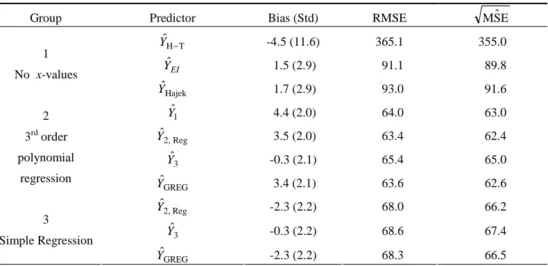
The main conclusions from Tables 1.1 – 1.3 are as follows: 1- All the predictors considered for this study are virtually

design unbiased with all three sample sizes, irrespective of the underlying working model. The predictor Yˆ₁ has a statistically significant bias when tested by use of the conventional t-statistic but the actual bias is negligible when compared to the true population total. (The predictor Yˆ₁ is the only predictor considered in this study that is not design consistent).

[image:10.612.74.541.92.342.2]

2- The predictors in Groups 2 and 3 that use the auxiliary values perform much better than the predictors in Group 1, particularly for the smaller sample sizes. The pre-dictors in Group 2 that employ the 3rd order polynomial regression model (7.1) perform better than the corre-sponding predictors in Group 3 that employ the simple regression model as the working model, but the dif-ferences diminish as the sample size increases.

3- An important result emerging from this study is that the predictors Yˆ_2,Reg and Yˆ_EI (and also Yˆ₃ for the larger sample sizes), that only predict the y-values for units outside the sample indeed perform better than the other predictors in their respective groups (see also below). As surmised in Remark 7, this holds particularly with the larger sample sizes. Notice that the differences between

Reg , 2

ˆ

Y and the GREG estimator for n =1,145 and n =2,250 are smaller under the polynomial model (Group 2) than under the simple regression model (Group 3), which is explained by the tight relationship between the study variable and auxiliary variables under the polynomial model. The predictor Yˆ₃ is less stable than Yˆ_2,Reg for n = 232 but for the other two sample sizes the two predictors perform similarly.

4- The predictor Yˆ_2,Reg performs somewhat better than the model dependent predictor Yˆ₁ that employs the expectations E(w_i |x_i) to adjust the sampling weights. We have no clear explanation for this result because as illustrated in Pfeffermann and Sverchkov (1999) using

the same data, adjusting the sampling weights improves the estimation of the regression coefficients very significantly.

Next consider the MSE estimators.

5- The MSE estimators developed in section 6 perform very well for all the predictors and with all the sample sizes. For the sample size n = 232 there is a systematic under-estimation of the RMSE by up to 3%, which is explained by the fact that the pseudo population is in this case less variable than the actual study population (see Remark 9). The MSE estimators are almost unbiased for the other sample sizes with the largest difference between the estimated and true RMSE being again in the magnitude of 3%.

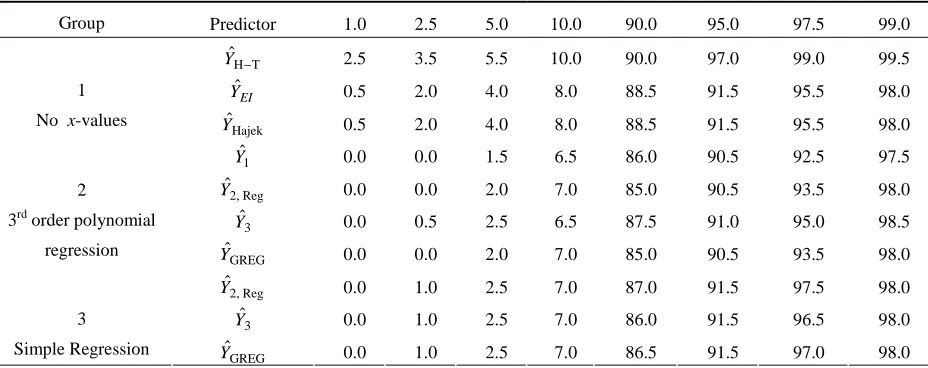
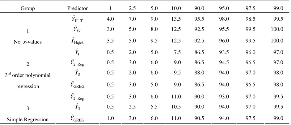
Another way of assessing the bias of the various predictors and their MSE estimation is by studying the coverage properties of confidence intervals defined by these predictors. Tables 2.1 – 2.3 compare the empirical percentage coverage of the standard confidence intervals

±

Yˆ Z_1−α/2 MSˆE with the corresponding nominal percentages for selected values of α (one table for each sample size). The empirical percentages are somewhat erratic with n = 232 sample units but they stabilize as the sample size increases, particularly with the use of the predictors in the second and third group. The empirical percentages are close to the nominal percentages with all the predictors when n = 2,250.

[image:11.612.112.507.484.676.2]

Table 1.1

Bias, RMSE and Square Root of Mean of MSE Estimators, n = 232

Group Predictor Bias (Std) RMSE EMSˆ

T H

ˆ

−

Y -4.5 (11.6) 365.1 355.0

EI

Yˆ 1.5 (2.9) 91.1 89.8

1 No x-values

Hajek

ˆ

Y 1.7 (2.9) 93.0 91.6

1

ˆ

Y 4.4 (2.0) 64.0 63.0

Reg , 2

ˆ

Y 3.5 (2.0) 63.4 62.4

3

ˆ

Y -0.3 (2.1) 65.4 65.0

2 3rd order polynomial

regression

GREG

ˆ

Y 3.4 (2.1) 63.6 62.6

Reg , 2

ˆ

Y -2.3 (2.2) 68.0 66.2

3

ˆ

Y -0.3 (2.2) 68.6 67.4

3 Simple Regression

GREG

ˆ

Y -2.3 (2.2) 68.3 66.5

[image:12.612.112.507.93.277.2]

Table 1.2

Bias, RMSE and Square Root of Mean of MSE Estimators, n = 1,145

Group Predictor Bias (Std) RMSE EMSˆ

T H

ˆ

−

Y -9.1 (5.0) 157.1 156.1

EI

Yˆ 0.0 (1.1) 35.2 34.9

1 No x-values

Hajek

ˆ

Y -0.1 (1.3) 39.5 39.3

1

ˆ

Y 3.0 (0.9) 27.6 28.1

Reg , 2

ˆ

Y 2.0 (0.9) 27.4 27.3

3

ˆ

Y 0.5 (0.9) 27.4 27.7

2 3rd order polynomial

regression

GREG

ˆ

Y 1.7 (0.9) 27.8 27.8

Reg , 2

ˆ

Y 0.0 (1.0) 28.3 28.7

3

ˆ

Y 0.1 (1.0) 28.2 28.9

3 Simple Regression

GREG

ˆ

Y 0.0 (2.0) 29.1 29.6

[image:12.612.106.512.324.506.2]

True ‘population’ total= 2710.7

Table 1.3

Bias, RMSE and Square Root of Mean of MSE Estimators, n=2,250

Group Predictor Bias (Std) RMSE EMSˆ

T H

ˆ

−

Y 1.3 (2.7) 82.7 80.4

EI

Yˆ -0.2 (0.6) 18.5 18.8

1 No x-values

Hajek

ˆ

Y 0.1 (0.7) 23.5 23.8

1

ˆ

Y 1.3 (0.5) 17.5 17.3

Reg , 2

ˆ

Y 0.6 (0.5) 16.9 16.3

3

ˆ

Y -0.3 (0.5) 17.1 16.5

2 3rd order polynomial

regression

GREG

ˆ

Y 0.5 (0.5) 17.9 18.3

Reg , 2

ˆ

Y -0.3 (0.5) 17.3 16.8

3

ˆ

Y -0.3 (0.5) 17.7 17.3

3 Simple Regression

GREG

ˆ

Y -0.2 (0.6) 18.8 18.3

True ‘population’ total= 2710.7

Table 2.1

Nominal and Empirical Percentage Coverage of Confidence Intervals, n = 232

Group Predictor 1.0 2.5 5.0 10.0 90.0 95.0 97.5 99.0

T H

ˆ

−

Y 2.5 3.5 5.5 10.0 90.0 97.0 99.0 99.5

EI

Yˆ 0.5 2.0 4.0 8.0 88.5 91.5 95.5 98.0

1 No x-values

Hajek

ˆ

Y 0.5 2.0 4.0 8.0 88.5 91.5 95.5 98.0

1

ˆ

Y 0.0 0.0 1.5 6.5 86.0 90.5 92.5 97.5

Reg , 2

ˆ

Y 0.0 0.0 2.0 7.0 85.0 90.5 93.5 98.0

3

ˆ

Y 0.0 0.5 2.5 6.5 87.5 91.0 95.0 98.5

2 3rd order polynomial

regression

GREG

ˆ

Y 0.0 0.0 2.0 7.0 85.0 90.5 93.5 98.0

Reg , 2

ˆ

Y 0.0 1.0 2.5 7.0 87.0 91.5 97.5 98.0

3

ˆ

Y 0.0 1.0 2.5 7.0 86.0 91.5 96.5 98.0

3

[image:12.612.76.540.554.738.2]

[image:13.612.72.543.93.296.2]

Table 2.2

Nominal and Empirical Percentage Coverage of Confidence Intervals, n = 1,145

Group Predictor 1 2.5 5.0 10.0 90.0 95.0 97.5 99.0

T H

ˆ ₋

Y 4.0 7.0 9.0 13.5 95.5 98.0 98.5 99.5

EI

Yˆ 3.0 5.0 8.0 12.5 92.5 95.5 99.5 100.0

1

No x-values YˆHajek 3.5 5.0 9.5 12.5 92.5 96.0 99.5 100.0

1

ˆ

Y 0.5 2.0 5.0 7.5 86.5 93.5 96.0 97.0

Reg , 2

ˆ

Y 0.5 3.0 6.0 9.0 86.5 94.5 96.5 97.0

3

ˆ

Y 0.5 2.0 6.0 9.5 88.0 94.0 97.0 98.0

2

3rd order polynomial

regression YˆGREG 0.5 3.0 5.0 9.0 86.5 94.0 96.5 98.0

Reg , 2

ˆ

Y 0.5 3.0 6.0 11.0 90.0 93.0 97.0 99.5

3

ˆ

Y 0.5 2.5 5.5 10.5 90.0 94.0 97.0 99.5

3

[image:13.612.77.541.335.536.2]

Simple Regression YˆGREG 1.0 3.0 6.0 11.0 90.5 94.0 97.5 99.0

Table 2.3

Nominal and Empirical Percentage Coverage of Confidence Intervals, n = 2,250

Group Predictor 1.0 2.5 5.0 10.0 90.0 95.0 97.5 99.0

T H

ˆ

−

Y 0.5 1.0 5.5 11.0 95.0 97.5 99.0 99.5

EI

Yˆ 1.0 3.0 5.5 9.0 91.5 96.0 99.0 99.5

1

No x-values YˆHajek 1.0 2.5 5.5 9.0 93.0 97.0 98.5 99.5

1

ˆ

Y 0.5 2.0 5.0 9.0 91.0 94.5 96.5 97.5

Reg , 2

ˆ

Y 0.5 2.5 6.5 10.5 90.5 94.5 96.5 98.0

3

ˆ

Y 0.5 2.0 7.5 12.5 91.5 95.5 96.5 97.5 2

3rd order polynomial

regression YˆGREG 0.5 2.0 6.0 11.0 91.0 94.5 96.0 98.0

Reg , 2

ˆ

Y 1.0 3.0 6.0 11.0 91.0 95.0 97.5 99.0

3

ˆ

Y 1.0 2.0 6.0 12.0 90.0 95.0 97.5 98.0 3

Simple Regression YˆGREG 0.0 1.5 5.0 11.5 91.5 95.0 97.5 99.0

As implied by the theoretical developments of this article and illustrated in the empirical study, predicting only the y-values for units outside the sample employing the sample-complement model yields better predictors for the population total than predicting all the population values by use of the population model, as implicitly implemented when using the GREG or Hajek’s estimators. Clearly, the differences are only appreciable when the sampling fractions are not negligible.

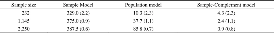
In order to highlight this point further, we present in Table 3 the mean prediction error (mpe) in the original scale (grams) over the 1,000 samples when predicting the sample-complement values;

[

(ˆ ) ( )

]

1,000 mpe=

∑ ∑

1_r,₌000_{1 j∉S j} − _j −

k

n N y y

where S_r defines the rth selected sample. The mpe’s are shown for three predictors, all utilizing the working model (7.1) and thus having the general form, yˆ_j =βˆ₀+

. , βˆ βˆ

βˆ 3

3 2 2

1xj + xj + xj j∉s For the first predictor the

[image:14.612.67.544.104.162.2]

Table 3

Mean Prediction Errors and Std of Means (in brackets) Under Three Prediction Models

Sample size Sample Model Population model Sample-Complement model

232 329.0 (2.2) 10.3 (2.3) 4.3 (2.3)

1,145 375.0 (0.9) 37.7 (1.1) 2.4 (1.1)

2,250 387.5 (0.6) 85.8 (0.7) 0.9 (0.8)

The clear conclusion emerging from Table 3 is that the use of either the population model or the model holding for units in the sample for the prediction of y-values of units outside the sample can result in appreciable biases. Notice that the bias induced by use of the population model increases as the sampling fraction increases, which agrees with the previous discussion asserting that the difference between the sample and sample-complement models only shows up with relatively large sample sizes (see Comment 2).

8. CONCLUDING REMARKS

In this article we use the sample and sample-complement distributions for developing design consistent predictors of finite population totals. Known predictors in common use are shown to be special cases of the present theory. The MSEs of the new predictors are estimated by a combination of an inverse sampling algorithm and a resampling method. As supported by theory and illustrated in the empirical study, predictors of finite population totals that only require the prediction of the outcome values for units outside the sample perform better than predictors in common use even under a design based framework, unless the sampling fractions are very small. The MSE estimators are shown to perform well both in terms of bias and when used for the computation of confidence intervals for the population totals. Further experimentation with this kind of predictors and MSE estimation is therefore highly recommended.

ACKNOWLEDGEMENT

The authors would like to thank the associate editor and two referees for very constructive comments.

REFERENCES

BREWER, K.R.W. (1963). Ratio estimationand finite populations: some results deducible from the assumptions of an underlying stochastic process. Australian Journal of Statistics. 5, 93-105.

BREWER, K.R.W. (1999). Cosmetic calibration with unequal probability sampling. Survey Methodology. 25, 205-212. CHAMBERS, R.L., DORFMAN, A. and SVERCHKOV, M.

(2003). Nonparametric regression with complex survey data. In, Analysis of Survey Data, (Eds. C. Skinner and R. Chambers). New York: John Wiley & Sons, Inc. 151-174.

FULLER, W. (2003). Statistical analysis from complex survey data. Tutorial presented at the International Statistical Institute meeting, Berlin, Germany. Slides of the Tutorial appear in http://cssm.iastate.edu/academic/ staff/fuller.html.

HANSEN, M.H., MADOW, W.G. and TEPPING, B.J. (1983). An evaluation of model-dependent and probability-sampling inferences in sample surveys (with discussion). Journal of the American Statistical Association.. 78, 776-807.

KIM, D.H. (2002). Bayesian and empirical Bayesian analysis under informative sampling. Sankhyā B. 64, 267-288.

KORN, E.L., and GRAUBARD, B.I. (1995). Examples of differing weighted and unweighted estimates from a sample survey. The American Statistician. 49, 291-295.

PATAK,