Abstract—This paper studies the optimal collision avoidance strategies in a close proximity coplanar cooperative encounter between two participants with equal linear speeds, but unequal turn capabilities. The synthesis of optimal control can be presented in the form of a 2D diagram with dispersal curves partitioning the plane of the initial relative positions into sub-regions of initial positions for different optimal strategies. To resolve the non-uniqueness of the optimal strategies associated with the dispersal curves, the maneuver time is introduced as an additional performance criterion. We show that, while in the case of an encounter of identical participants the optimal collision avoidance strategies that start at the dispersal point often have identical maneuver time, this is no longer the case when the participants have unequal turn capabilities. We show that a unique strategy with a smaller maneuver time can be identified based on the non-dimensional parameter of the problem. Efficient numerical algorithms for calculation of the maneuver time for optimal strategies are presented. The results in this paper are applicable in aviation and marine collision avoidance and in robotics applications.
Index Terms — Optimal control, Collision avoidance, Cooperative maneuvers, Dispersal curves, Maneuver time
I. INTRODUCTION
Encounters, where the participants are sufficiently close in space and time to be of operational concern (they are often called close proximity encounters), can occur in many applications in aviation, navigation and robotics. The optimal cooperative collision avoidance strategies for a coplanar close proximity encounter between two identical participants was first studied by Merz [1], [2] (a rigorous analysis is given in [3]). Recently, the analysis has been extended for an encounter of participants with unequal turn capabilities, but with equal linear speeds [4-6].
In [1-6], the synthesis of the optimal control solution is presented in the form of a 2D diagram which establishes the optimal collision avoidance strategy for both participants based on their initial relative position and relative orientation. Such a diagram presents an important tool for setting and validating the traffic rules, and also for testing and validating
Manuscript received October 29, 2010.
T. Tarnopolskaya is with the Commonwealth Scientific and Industrial Research Organisation (CSIRO), Mathematics, Informatics and Statistics, Locked Bag 17, North Ryde, NSW 1670, Australia (phone: +61 2 9325 3254; fax+61 2 9325 3200; e-mail: [email protected]).
N. L. Fulton is with the Commonwealth Scientific and Industrial Research Organisation (CSIRO), Mathematics, Informatics and Statistics, Canberra, ACT 2601, Australia (e-mail: [email protected]).
automatic collision avoidance systems.
There is a vast body of literature devoted to the optimal resolution of conflicts and optimal control for aviation and marine collision avoidance applications and for robotics (the references [7-32] are just a few examples). While an advance in numerical optimization techniques makes it possible to study complex scenarios involving many participants, analytic and semi-analytic synthesis of optimal control solutions of the type developed in [1-6] are still important, as they provide an insight into the underlying structure of the solution and can be used as benchmarks against which numerical solutions can be compared.
This paper continues the study in [1-6] and focuses on the dispersal curves for the case of participants with unequal turn capabilities. A dispersal curve (which is a planar case of a dispersal or singular surface in differential games theory [33]) separates the regions of different optimal strategies. Such a curve presents a locus of the initial positions for which an optimal solution is not unique (i.e., there are two optimal strategies that result in the same terminal miss distance). In the case of the coplanar close proximity encounter, there is also a triple point present, where the three optimal strategies result in the same terminal miss distance. Dispersal curves and the triple point therefore involve conflicting decisions for the participants as to which of equally optimal paths to take.
This paper introduces an additional performance criterion that can be used to select a unique optimal strategy that originates at a dispersal point or at the triple point. Such a criterion is the maneuver time, which is not only important in a theoretical sense as a measure of efficiency, but also in a practical sense as an input to a flight management / autopilot system design.
The main results of the paper can be summarized as follows. We have shown for the case of identical participants that the maneuver times for two optimal strategies originating at a dispersal point are often identical; this is not the case for participants with unequal turn capabilities. We show that a unique strategy for participants with unequal turn capabilities can be selected if the maneuver time is considered as an additional performance criterion. A simple analytic characterization of the unique strategy with the smaller maneuver time is established. Efficient numerical algorithms for calculation of the maneuver time are also presented. Only the RR-LL dispersal curve and the triple point are considered, as they are situated in the region of smaller relative distance between the participants, and therefore are of main concern in a close proximity encounter. However, it is straightforward to
Non-unique Optimal Collision Avoidance
Strategies for Coplanar Encounter of Participants
with Unequal Turn Capabilities
Tanya Tarnopolskaya, Neale L. Fulton
IAENG International Journal of Applied Mathematics, 40:4, IJAM_40_4_10
extend the analysis to other dispersal curves.
This paper is an extended and revised version of the conference paper [6].
II. OPTIMIZATION PROBLEM
The assumptions adopted in this paper are the same as in the close proximity encounter models [1]-[5]. Thus, we assume that the linear speeds of the participants are constant. The maximization of the terminal miss distance (which is a minimal distance between the participants during the maneuver) is adopted as the performance criterion.
The nondimensional equations of motion of the two participants with equal linear speeds but unequal turn capabilities in the moving polar coordinate system are [1]-[5]
1
1 2
cos cos( )
[sin sin( )] /r f( , ),u
φ θ φ
ρ σ φ θ φ ρ
σ ωσ
− + −
= − + + − ≡
− +
ɺ (1)
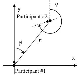
where ρT =( , , )r φ θ ; , ,r φ θ specify the non-dimensional instantaneous relative distance between the participants and the instantaneous angles defining the relative direction of their motion (see Fig. 1), r:=r R/ 1min, R1min is the lower bound on the turn radius of the first participant; σ σ1, 2are the non-dimensional angular speeds of the participants scaled so that they are contained in the interval [-1, 1], with positive values corresponding to the right turns (from the point of view of the participant), and negative values corresponding to the left turn, σ1=ω ω1/ 1max, σ2 =ω ω2/ 2max, where ω ω1, 2are the angular speeds, ω1max,ω2max are the absolute values of physical bounds on the angular speeds of the participants; ω is the non-dimensional parameter of the problem,
max max 2 / 1 0.
ω ω= ω > The derivatives with respect to the non-dimensional time t t( :=tω1max )are denoted with dots. The domains for the variables ,φ θare defined as
, π φ π
− ≤ < 0≤ <θ 2 .π
The system of ordinary differential equations (1) can be viewed as a control system with the state vector
( , , )
T r
ρ = φ θ and control function uT =(σ σ1, 2), 2
: [0, ]→ ; ⊆ , = −[ 1, 1] [ 1, 1].× −
u T U U R U
The non-dimensional maneuver time T (also known as the terminal time) is defined as the time to closest approach between the participants. It is defined by the conditions
( ) 0,
r Tɺ = (2) ( )<0 for ∈[0, ].
ɺ
r t t T (3) The objective is to maximize the terminal miss distance
( , )u rt T rT
ψ ρ = = ≡ over all admissible controls. Thus, the performance index is a function of the terminal time only. As the terminal time
T
is unknown, the problem can be considered as a Mayer problem with free terminal point.By substituting the expression for rɺ from the first equation of (1) into the terminal condition (2), it is easy to see that the terminal condition (2) splits into two equations
sin(θT/ 2)=0, sin(φ θT− T/ 2)=0, which yield two terminal conditions:
1. θT =0; (4)
2. φT =θT/2−π, φT =θT/2. (5)
III. NECESSARY CONDITIONS FOR NONSINGULAR OPTIMAL
CONTROLS
The Hamiltonian function in the polar coordinate system is given by:
1 2
1
( , , ) ( , )
[ cos cos( )] ( )
{ [sin sin( )] / },
θ φ
λ ρ λ ρ
λ φ θ φ λ σ ωσ
λ σ φ θ φ
=
= − + − + − +
+ − + + −
i
T
r
H u f u
r
(6)
where the adjoint variables λT ≡(λ λ λr, ϕ, θ) satisfy the equationsλɺ = −∇H, that is
2 [sin sin( )] /
(sin sin( )) [cos cos( )] /
sin( ) cos( ) /
r
r
r
r r
φ
φ φ
λ φ θ φ
λ λ φ θ φ λ φ θ φ
λ θ φ λ θ φ
+ −
= − + − − − −
− + −
ɺ (7)
subject to
( )T ( ( ), )T u [1, 0, 0]T
λ = ∇ψ ρ = . (8) Using the Pontryagin Maximum Principle [34], [35], together with the terminal conditions (4), (5), and adjoint equations (7), (8), it can be shown ([3], [4]) that there are two types of possible optimal strategies at the terminal time: 1) terminal condition (4) corresponds to σ1=−σ2=±1 (the participants are turning with maximum possible angular speeds in an opposite directional sense). We will call such strategies the right-left (RL) and the left-right (LR) strategies, where the first letter indicates the strategy of the first participant (located in the origin of Fig.1); 2) terminal condition (5) results in σ1=σ2 =±1 (both participants are turning in the same directional sense with maximum possible angular speeds). Such strategies will be called the right-right (RR) and the left-left (LL) strategies.
Using the transformation of variables 2 2
y x
r = + ,
,
sin x
[image:2.595.356.490.50.179.2]r φ= rcosφ=y, (1) can be re-written in the Cartesian coordinates and presented in terms of backward (retrograde)
Figure 1: Schematics of the coplanar encounter in the moving coordinate system
φ
r
θ
x y
Participant #1 Participant #2
IAENG International Journal of Applied Mathematics, 40:4, IJAM_40_4_10
derivatives as
1 sin , 1 1 cos , 1 2,
x =σ y− θ y = −σx− θ θ σ ωσ = − (9) where circles denote the derivative with respect to τ
(τ = −T t ).
Solving (9) subject to the conditions
0 T,
xτ= =x 0 T,
yτ= =y and each of the two terminal conditions (4), (5) in turn yields the following two cases for the extremals: Case I. θT =0, σ1=−σ2=±1. This case corresponds to the RL and LR strategies. The solution of (9) is given by
1 1
1 1
1 1
1
(1 ) for 1,
2 (1 ) for 1,
sin( ) [1 cos[(1 ) ] /
(1 ) cos / ],
cos( ) (1 ) sin /
sin[(1 ) ] / ,
T T
T T
x r
y r
σ ω τ σ
θ π σ ω τ σ
φ σ τ σ ω τ ω
ω τ ω
φ σ τ ω τ ω
ω τ ω
+ =
=
+ + = −
= + + + +
− +
= + + +
− +
(10)
where subscript “T” refers to the terminal instant. For τ =T, (10) describes the locus of the initial conditions
) ,
(
0 0 0
0 ≡xt= y ≡yt=
x for the RL and LR strategies and takes
the form
For σ1=1:
2
0 0 0
2 2
0 0 0
{ 1 cos / (1 ) cos[ / (1 )] / } { (1 ) sin[ / (1 )] / sin / } T,
x
y r
θ ω ω θ ω ω
ω θ ω ω θ ω
− − + + +
+ − + + + = (11)
For σ1=−1:
0 0
2
0 0 0
2 2 0
{ (1 ) cos[( 2 ) / (1 )] / 1
cos / } { (1 ) sin[( 2 ) / (1 )] / sin / } T.
x
y
r
ω θ π ω ω
θ ω ω θ π ω ω
θ ω
− + − + +
+ + + + − +
− =
(12)
One can see that, for given θ ω0, and rT, the loci of the initial relative positions (11), (12) for the RL and LR strategies respectively represent circles.
Case II. θT =2φT +2π or θT =2φT; σ1=σ2=±1. This
case corresponds to the RR and LL strategies. The solution of (9) takes the form
1
1
1 1 1
1 1 1
1 1 1
(1 ) , cos( ) sin
{sin( ) sin[ (1 ) ]} / , sin( ) cos( ) /
(1 cos ) cos[ (1 ) ] / .
T
T T
T T
T T T
T
y r
x r
θ σ ω τ θ
φ σ τ τ
σ θ σ τ θ σ ω τ ω
φ σ τ σ θ σ τ ω
σ τ σ θ σ ω τ ω
= − +
= + +
− + − + −
= + + +
+ − − + −
(13)
Forτ=T we have θ0=σ1(1−ω)T+θT,and the locus of
the initial conditions (x0≡xt=0,y0 ≡yt=0) for the RR and LL
strategies is given by: Forφ =T θT /2:
2 2
0 1 0 0 1 0
2
0 1
1 0 1
[ (1 cos / )] ( sin / ) 2 2 cos[ (1 ) ] /
2 (1 1 / ) sin[( (1 ) ) / 2],
σ θ ω σ θ ω
θ σ ω ω
σ ω θ σ ω
− − + −
= + − − −
− + − −
T
T
x y
r T
r T
(14)
ForφT =θT /2−π :
2 2
0 1 0 0 1 0
2
0 1
1 0 1
[ (1 cos / )] ( sin / ) 2 2 cos[ (1 ) ] /
2 (1 1 / ) sin[( (1 ) ) / 2].
σ θ ω σ θ ω
θ σ ω ω
σ ω θ σ ω
− − + −
= + − − −
+ + − −
T
T
x y
r T
r T
(15)
For given θ ω0, and rT , the loci of the initial relative positions for the RR and LL strategies (14) and (15) represent arcs of spirals.
IV. SYNTHESIS OF OPTIMAL CONTROL
First, consider the locus of points on the plane of the initial relative positions satisfying rɺt=0 =0. This locus is called in [3], [4] an initial zero range rate line. It partitions the plane of the initial relative positions ( , )x y into the regions
0 0
= >
ɺt r
(diverging relative distance) and
0 0
= <
ɺt
r (converging
relative distance) at the beginning of the maneuver. Condition (3) implies that the optimal trajectories can only start in the region of converging relative distance
0 0.
= <
ɺt
r The
following property follows from the terminal condition (2): Property 1 A straight line passing through the origin withtanφ =tan(θ0/2) represents the locus rɺt=0 =0.
In a similar manner, the locus rɺt T= =0is called in [3], [4] a terminal zero range rate line. It follows from the first of Eqs. (13) and terminal conditions (5) that:
Property 2 Straight lines passing through the origin with
0 1 1
tanφT =tan{[θ σ− (1−ω) ] / 2},T σ = ±1, (16) represent the loci 0
t T
rɺ = = for the RR and the LL strategies. For given θ0 and ω, the RR and LL trajectories end on lines (16).
The first step toward identifying the optimal strategy is to identify the trajectories from the sets of extremals (10), (13), such that the distance between the participants decreases on the time interval t∈[0,T] (i.e., condition (3) is satisfied). The following property holds [4]:
Property 3 For the loci of initial relative positions (15) with
1 1
σ = and (14) with σ1= −1 , there exists an interval [0, ],ε ε >0, such that the trajectories with T∈[0, ]ε have decreasing relative distance.
The synthesis of optimal control can be constructed as follows (for details, see [3], [4]):
• for a given θ0,rTand ω, select the trajectories from the sets of extremals (10), (13), such that the distance between the participants decreases on the time interval
] , 0 [ T
t∈ (i.e., condition (3) is satisfied);
• for a given θ0,rTand ω, construct the loci of the initial relative positions with associated strategies that correspond to the trajectories with decreasing distance between the participants on t∈[0,T];
• for the loci constructed in the previous step, construct the internal envelope (i.e., the locus of points that are closest to the origin for each value of φ); this envelope consists of the initial positions for different nonsingular strategies. It can be shown (see [4]) that the strategies associated with the internal envelope are the optimal
IAENG International Journal of Applied Mathematics, 40:4, IJAM_40_4_10
strategies for given θ0,rTandω;
For given rT,θ0 ( 0<θ <0 π ) andω , the internal
envelope consists of the arcs of the loci of the initial positions for the RR strategy (15) (σ1=1), the LL
strategy (14) (σ1=−1) and, for certain values of rT, also
contains the arc of the locus of the initial conditions for the RL strategy (11);
• finally, extend the internal envelope for all values of rT. As a result of this procedure, the half-plane of initial relative positions that correspond to trajectories with initially converging relative distance is partitioned into the sub-regions of initial relative positions for different optimal strategies, with dispersal curves separating them.
Below, we summarize several results from [4] that are useful for the analysis in this paper.
• For 0<θ <0 π , there are three sub-regions of initial relative positions for optimal strategies: the sub-region of the initial positions for the right-right (RR) strategy (called the RR locus for brevity); the sub-region of initial positions for the left-left (LL) strategy (the LL locus), and the sub-region of the initial positions for the right-left (RL) strategy (the RL locus). Forπ <θ0 <2π, the three
sub-regions are the RR, the LL and the LR loci;
• For 0<θ <0 π , there exists a value of the terminal miss distance rT =rTtp such that the points on the internal envelope that correspond to the initial relative positions for the RR, LL and RL strategies have a common intersection point. Such point is called a triple point; • For any rT <rTtp, the internal envelope does not contain
the points that correspond to the initial conditions for the RL or LR strategies; the points on the internal envelope that correspond to the initial relative positions for the RR and LL strategies intersect at a point that is called the RR-LL dispersal point;
• For anyrT >rTtp, the points on the internal envelope that correspond to the initial relative positions for the RR and RL strategies intersect at a point that is called the RR-RL dispersal point; the points on the internal envelope that correspond to the initial relative positions for the LL and RL strategies intersect at the LL-RL dispersal point. The RR-RL and the LL-RL dispersal points do not coincide; • The optimal trajectory will never leave the locus of the initial relative positions corresponding to a given optimal strategy if it started in this locus;
• The strategies that include singular controls are suboptimal.
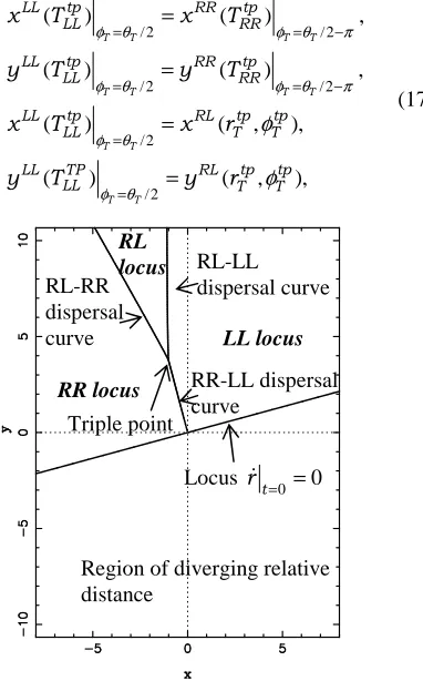
The synthesis of optimal control diagram presented in Figure 2 shows the typical structure of the synthesis. The plane of the initial relative positions, at the initial time, is partitioned by the zero range rate line (the locus
0 0 t
rɺ = = ) into two half-planes of initial relative positions for trajectories with diverging and converging relative distance respectively. The half-plane of initial relative positions for trajectories with converging relative distance is further separated into three regions of initial relative positions with each region
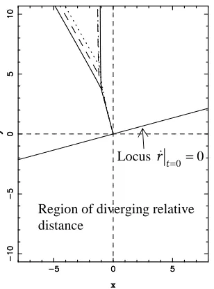
corresponding to a different optimal strategy. The dispersal curves separate these regions. For 0<θ0<π,there are three dispersal curves: the RR-LL, the RL-LL and the RL-RR dispersal curves. They separate the half-plane of converging relative distance into the loci of the initial relative positions for the RR, the LL and the RL optimal strategies (we call them the RR, LL and RL loci respectively for brevity). A triple point (i.e. the point on the plane of initial relative positions such that the RR, LL and RL strategies that start at this point result in the same terminal miss distance) is also illustrated in Fig. 2. Note that the synthesis of the optimal control diagram for identical participants shown in Fig.2 is characterized by the symmetry of the dispersal curves with respect to the RR-LL dispersal curve (which in case of identical participants represents a straight line). For the case of an encounter of participants with unequal turn capabilities, the synthesis of optimal control diagram is shown in Fig. 3. While the zero range rate line remains unchanged for different values of ω in this case, the dispersal curves shift clockwise. Thus, the symmetry of the synthesis of the optimal control diagram is lost.
V. DISPERSAL CURVES AND TRIPLE POINT
In what follows, we only consider the case 0< <θ0 π for the sake of brevity, and show how the triple point and the dispersal curves can be calculated. To find the triple point, one needs to find, for given θ0,rT andω, the point of intersection of the loci of the initial relative position for the LL strategy, the RR strategy and the RL strategy that result in the trajectories with decreasing relative distance. Thus, one needs to satisfy the conditions
/ 2 / 2
/ 2 / 2
/ 2
/ 2
( ) ( ) ,
( ) ( ) ,
( ) ( , ),
( ) ( , ),
T T T T
T T T T
T T
T T
tp tp
LL RR
LL RR
tp tp
LL RR
LL RR
tp tp tp
LL RL
LL T T
tp tp
LL TP RL
LL T T
x T x T
y T y T
x T x r
y T y r
φ θ φ θ π
φ θ φ θ π
φ θ
φ θ
φ
φ
= = −
= = −
=
=
=
=
=
=
[image:4.595.352.543.450.757.2](17)
Figure 2: Synthesis of optimal control diagram,
0 5 / 6; 1.
θ = π ω=
Region of diverging relative distance
RR-LL dispersal curve
RL-LL dispersal curve RL-RR
dispersal curve
Triple point Locus
0 0 t
rɺ = = LL locus
RR locus RL locus
IAENG International Journal of Applied Mathematics, 40:4, IJAM_40_4_10
where TLLtp and TRRtp are the maneuver times for the LL and the RR strategies at the triple point respectively. The terminal miss distance and the terminal relative bearing at the triple point are rTtp and φTtprespectively. Conditions (17) can be reduced to the following system of three trigonometric equations 0 0 0 0 0 0 0 0
0 sin(( ) / 2) 2 cos / sin(( ) / 2) cos 2 cos [cos( ) cos( )] / , 0 cos(( ) / 2) 2sin /
cos(( ) / 2) sin
tp tp tp
LL LL T
tp tp tp tp
RR RR LL
T
tp tp tp
RR LL RR
tp tp tp
LL LL T
tp tp tp tp
RR RR LL
T
r T T
r T T T
T T T
r T T
r T T T
θ ω θ ω
θ ω
θ ω θ ω ω
θ ω θ ω
θ ω = − − + + + + + − + − − + + = − − − + + + + 0 0 2 0 2 0 0 0 0
sin [sin( ) sin( )] / , ( ) { sin(( ) / 2) cos 2
cos( ) / ( 1) cos( / (1 )) / } { cos(( ) / 2) sin 2 sin( ) / ( 1) sin[
tp tp tp
RR LL RR
tp tp tp tp tp
LL LL LL
T T
tp LL
tp tp tp tp
LL LL LL
T
tp LL
T T T
r r T T T
T
r T T T
T
θ ω θ ω ω
θ ω
θ ω ω ω θ ω ω
θ ω
θ ω ω ω
− + − + +
= − − + −
− − + + +
+ − − + −
+ − − + 2
0/ (1 )] / } ,
θ +ω ω
(18)
with the unknowns (TLLtp,TRRtp,rTtp). The initial guesses for the unknowns are obtained from the corresponding values for identical participants (ω = 1) [4]
,1 ,1 0
,1
0
2sin( / 2) arccos ,
[ 2sin( / 2)]
tp tp
LL RR tp
T T T r θ θ = = + (19) 2 ,1 0 0 0
(1 cos( / 2)) sin( / 2) cos( / 2) 1 tp T r θ θ θ − =
+ − . (20) Equations (18) are solved incrementally, starting with ω=1, until the value of interest is reached, updating the initial guess at each step. Using the calculated values(TLLtp,TRRtp,rTtp), the coordinates of the triple point can then be computed from one of the equations (17).
We now consider the RR-LL dispersal curve for given
values of θ0 andω . This dispersal curve is of a special importance for a close proximity encounter as it corresponds to the smaller of the relative distances between the participants (see Figs. 2 and 3). To find the RR-LL dispersal point, one needs to find a point of intersection of the loci of initial relative position for the LL strategy (14) and of the loci of initial relative positions for the RR strategy (15). Thus, for a givenrT, one needs to find the maneuver times TLL and
RR
T for the LL and RR strategies so that
/ 2 / 2
( ) ( ) ,
T T T T
LL RR
LL RR
x T x T
φ θ= = φ θ= −π
/ 2 ( ) T T LL LL y T
φ θ= = ( ) T T/2
RR RR
y T
φ θ= −π.
These conditions can be written as the following system of two trigonometric equations with the unknown maneuver times(TLL,TRR)
0 0
0
0 0
0 1 0
0
0 0
0 sin(( ) / 2) 2 cos /
sin(( ) / 2) cos 2
cos [cos( ) cos( )] / ,
0 cos(( ) / 2 ) 2 sin /
cos(( ) / 2) sin sin
[sin( ) sin(
T LL LL
T RR RR LL
RR LL RR
T LL LL
T RR RR LL RR
LL RR
r T T
r T T T
T T T
r T T
r T T T T
T T
θ ω θ ω
θ ω
θ ω θ ω ω
θ ω θ ω
θ ω
θ ω θ ω
= − − +
+ + + + −
+ − − + +
= − − −
+ + + + −
+ − + + )] /ω−2.
(21)
The initial guesses for TLL and TRR can be obtained from the solution for identical participants (19). To construct a dispersal curve, one needs to solve (21) incrementally for the value of rT between 0 andrTtp. Once the maneuver times are found from (21), the RR-LL dispersal curve can be constructed using equations for either of the RR or LL loci of the initial relative positions.
To find the RL-LL dispersal point, one needs to find a point of intersection of the loci of the initial relative positions for the LL strategy (14) and the loci of initial relative positions for the RL strategy (11), that is
/ 2
( ) ( , ),
T T
LL RL
LL T T
x T x r
φ θ= = φ
/ 2 ( ) T T LL LL y T
φ θ= = ( , )
RL T T
y r ϕ .
These conditions can be reduced to a single trigonometric equation in TLL
2 0 2 0 0 0 2 0 0
{ sin[( ) / 2] 2 cos
1 (1 )
cos( ) cos[ / (1 )]}
{ cos[( ) / 2] sin
1 (1 )
sin( ) sin[ / (1 )]} .
T T LL LL LL
LL
T LL LL LL
LL
r r T T T
T
r T T T
T
θ ω
ω
θ ω θ ω
ω ω
θ ω
ω
θ ω θ ω
ω ω = − − − + + − − + + + − − + + + − − + (22)
The RL-RR dispersal point can be calculated in a similar manner by finding a point of intersection of the loci of initial relative positions for the RL (11) and the RR (15) strategies, which can then be reduced to solving a single trigonometric equation with the unknown TRR
2 0
0
2
0 0
( ) 1
{ sin cos( )
2
2 (1 )
cos cos[ / (1 )] cos }
RR RR
T T RR
RR
T T
r r T
T
θ ω θ ω
ω ω
θ θ ω
[image:5.595.100.254.68.276.2]ω ω + + = − + + + − + + −
Figure 3: Synthesis of optimal control diagram for different values ofω, θ0=5 / 6π .
Region of diverging relative distance
Locus
0 0 t
rɺ = =
IAENG International Journal of Applied Mathematics, 40:4, IJAM_40_4_10
0
0
2
0 0
( ) 1
{ cos sin( )
2
2 (1 )
sin sin[ / (1 )] sin } .
RR RR
T RR
RR
T T
r T
T
θ ω θ ω
ω ω
θ θ ω
ω ω
+ +
+ − − +
+
+ − + +
(23)
Equations (22) and (23) are solved iteratively, starting with the value of the terminal miss distance at the triple point
tp T T
r =r and using TLL =TLLtp (or TRR =TRRtp ) for a givenθ0 and ω as an initial guess. The value rT is then increased incrementally, while updating the initial guess for
LL
T (orTRR) at each step.
VI. MANEUVER TIMES FOR STRATEGIES THAT START AT THE
DISPERSAL OR TRIPLE POINT
Dispersal curves can be viewed as the loci of the initial relative positions that deliver a non-unique optimal strategy. This poses a problem in practical applications. By recognizing that, in the interest of efficiency of conflict resolution, a shorter maneuver time may be preferable, we now compare the competing strategies in order to identify the strategy that takes shorter time to implement.
The maneuver times TLL,TRR, as applicable for the strategies that originate at the RR-LL, RL-LL or RL-RR dispersal points, can be computed from (21), (22) and (23) respectively. The maneuver time for the strategies that originate at the triple point can be computed from (18). The maneuver time for RL strategy TRL is given by simple formula TRL =θ0/ (1+ω) (see first equation of (10)).
A. Identical Participants
First, we consider the case of identical participants. Proposition 1 For identical participants (ω=1), the RR and LL strategies, that start at the RR-LL dispersal point with a given terminal miss distancerT , have identical maneuver times given by
0 0
arccos{2sin( / 2) / [ 2sin( / 2)]}.
LL RR T
T =T = θ r + θ (24)
At the triple point, the maneuver times for the RR and LL strategies are identical, while the maneuver time for the RL strategy always exceeds that for the RR and LL strategies for
0 0<θ <π .
Proof For the case of identical participants, the RR-LL
dispersal curve is a straight line normal to the line 0 0 t
rɺ = =
(which is called a zero range rate line in [3]). The RR and LL loci of terminal positions in this case coincide with the locus
0 0. t
rɺ = = For a given rT , the RR and LL trajectories are the arcs of the circles that are symmetric relative to the RR-LL dispersal curve with centers on the zero range rate line (see [3] for details) and with a radius R r(T)=rT +2 sin(θ0/ 2). Simple geometric considerations give
0 0
cos( ) cos( ) [ ( ) ] / ( )
2sin( / 2) / [ 2sin( / 2)],
LL RR T T T
T
T T R r r R r
r
θ θ
= = −
= + (25)
which proves (24) .
It follows from (19), (20) and the first equation of (10) that the maneuver time for RL strategy is larger than the maneuver time for RR (or LL) strategy if
0 0 0
0
[1 cos( / 2)] / [(sin( / 2) cos( / 2) 1] 2 tan( / 2) 0.
θ θ θ
θ
− + −
− < (26)
It is straightforward to show that inequality (26) is valid for 0
0<θ <π □
The above results are illustrated in Fig.4, where the dispersal curves and the optimal trajectories for collision avoidance of identical participants are shown forθ0=2 / 3π . Note that, in case of an encounter of identical participants, the locus
0 0 t
rɺ = = coincides with the loci of terminal relative positions for both the RR and LL strategies, and we can see in Fig. 4 that the optimal RR and LL trajectories end on this locus. For the RL strategy that starts at the triple point, the circle of terminal relative positions is shown with a dotted line.
B. Participants with Unequal Turn Capabilities
The equality of the encounter times for the RR and the LL strategies in the case of an encounter of identical participants is the result of symmetry of the synthesis of optimal control diagram discussed in Section IV. For the case of participants with unequal turn capabilities, the symmetry is lost and the maneuver times for the strategies originating at the same dispersal point are never the same.
The maneuver times for the RR and the LL strategies starting at the RR-LL dispersal point are plotted in Fig.5 as functions of ω forθ0=2 / 3,π rT =1. We can see that the LL strategy takes longer to complete than the RR strategy forω>1, while the opposite is true for ω<1. The maneuver times coincide forω=1. Extensive numerical calculations show that such a
LL RR
1 2 3
4
5
Region of diverging relative distance
Locus
0 0 t
[image:6.595.62.286.53.102.2]rɺ = =
Figure 4: Dispersal curves and optimal trajectories, 0 2 / 3;
θ = π ω=1; 1 and 2 are the RR and LL optimal trajectories that start on the RR-LL dispersal point withrT =0.3, TLL =TRR =0.55; 3, 4 and 5 are RR, LL and RL trajectories respectively that start at the triple point withrTtp =0.683, TLL =TRR =0.771,
1.047 = RL
T .
IAENG International Journal of Applied Mathematics, 40:4, IJAM_40_4_10
[image:6.595.341.507.450.667.2]relationship between the maneuver times for the RR and LL strategies, that start at the RR-LL dispersal point, is typical for
0 0<θ <π .
Figures 6 and 7 show the RR-LL dispersal curves and the trajectories that start on these curves for ω>1 and ω<1 respectively. Note that for the encounter of participants with unequal turn capabilities, the locus 0 0
t
rɺ = = does not coincide with the loci of the terminal positions for the RR and LL strategies. These loci represent straight lines passing through the origin. They rotate anticlockwise for the LL and clockwise for the RR strategies respectively for ω>1, and
clockwise for the RR and anticlockwise for the LL strategies respectively for ω<1 (this behaviour is also illustrated in Figs. 6 and 7).
VII. CONCLUSIONS
This paper studies the optimal collision avoidance strategies associated with the dispersal curves and the triple point. Such strategies are essentially non-unique. We show that the issue of non-uniqueness of the optimal collision avoidance strategy starting at the dispersal point can be resolved for the case of participants with unequal turn capabilities, if the maneuver time is considered as an additional performance criterion. We prove that, for identical participants, the maneuver times for the RR and LL strategies that start at the RR-LL dispersal point (including the triple point) are equal. This is the result of the symmetry inherent in the synthesis of the optimal control diagram for the case of an encounter with identical participants. For identical participants, the RL strategy that starts at the triple point, always takes longer to complete than the RR or LL strategies. However, for the encounter of participants with unequal turn capabilities, the symmetry of the synthesis of the optimal control diagram is lost and the encounter times for the RR or LL strategies are never equal. The LL strategy that starts at the RR-LL dispersal curve takes longer to complete than the RR strategy forω>1, while the opposite is true forω<1.
[image:7.595.102.250.54.255.2]Thus, a unique optimal collision avoidance strategy with a smaller maneuver time can be identified based on the non-dimensional parameter of the problem ω. Efficient numerical algorithms for calculation of the maneuver time for optimal collision avoidance strategies are presented. The results in this paper are applicable in aviation and marine collision avoidance and robotics applications. Figure 5: Non-dimensional maneuver times for LL
(solid line) and RR (dashed-dotted line) strategies, that start at the RR-LL dispersal point, as functions of ω; θ0=2 / 3,π rT =1.
ω
1
2 RR-LL dispersal curve
RR locus of terminal positions LL locus of terminal positions
Locus 0 0
t
[image:7.595.346.503.55.265.2]rɺ = =
Figure 7: Dispersal curves and optimal trajectories forθ0 =5 / 6;π ω=0.5, 1 and 2 are the RR and LL optimal trajectories respectively that start on the RR-LL dispersal point withrT =0.6, TLL =0.8166,
0.8599 = RR
[image:7.595.91.241.492.698.2]T
Figure 6: Dispersal curves and optimal trajectories for
0 5 / 6; 4
θ = π ω= ; 1 and 2 are the RR and LL optimal trajectories respectively, that start on the RR-LL dispersal point with rT =0.6, TLL =0.4302,
0.3742 = RR
T .
1
2
Locus 0 0
t
rɺ = =
LL locus of terminal positions
RR locus of terminal positions
RR-LL dispersal curve
IAENG International Journal of Applied Mathematics, 40:4, IJAM_40_4_10
REFERENCES
[1] A. W. Merz, “Optimal aircraft collision avoidance”, Proc. Joint Automatic Control Conf., Paper 15-3, 1973, pp. 449-454.
[2] A.W. Merz, “Optimal evasive manoeuvres in maritime collision avoidance”, Navigation, vol. 20 (2), 1973, pp. 144-152.
[3] T. Tarnopolskaya, and N.L. Fulton, “Optimal cooperative collision avoidance strategy for coplanar encounter: Merz’s solution revisited”, J. Optim. Theory Appl., vol. 140 (2), 2009, pp. 355-375.
[4] T. Tarnopolskaya, and N.L. Fulton, “Synthesis of optimal control for cooperative collision avoidance for aircraft (ships) with unequal turn capabilities”, J. Optim. Theory Appl., vol. 144 (2), 2010, pp. 367-390. [5] T. Tarnopolskaya, and N.L. Fulton, “Parametric behavior of the optimal control solution for collision avoidance in a close proximity encounter”, In Anderssen, R.S. et al. (eds) 18th World IMACS Congress and MODSIM09 International Congress on Modelling and Simulation, July 2009, pp. 25-431. ISBN: 978-0-9758400 -7-8
[6] Tarnopolskaya, T., and Fulton, N.: Dispersal Curves for Optimal Collision Avoidance in a Close Proximity Encounter: a Case of Participants with Unequal Turn Rates. Lecture Notes in Engineering and Computer Science: Proceedings of The World Congress on Engineering 2010, WCE 2010, 30 June-2 July, 2010, London, U.K., pp. 1789-1794
[7] Miele, A., Wang, T., Mathwig. J.A., and Ciarcia, M.: Collision Avoidance for an Aircraft in Abort Landing: Trajectory Optimization and Guidance. J. Optim. Theory Appl. 146(2), 2010, pp. 233-254 [8] Miele, A., Wang, T., Chao, C.S., and Dabney, J.B.: Optimal Control of
a Ship for Collision Avoidance Maneuvers. J. Optim. Theory Appl. 103(3), 1999, pp. 495-518
[9] Miele, A., and Wang, T.: Optimal Trajectories and Guidance Schemes for Ship Collision Avoidance. J. Optim. Theory Appl. 129(1), 2006, pp. 1-20
[10] Miele, A., Wang, T., Chao, C.S., and Dabney, J.B.: Optimal Control of a Ship for Course Change and Sidestep Maneuvers. J. Optim. Theory Appl. 103(2), 1999, pp. 259-282
[11] Miloh, T., and Pachter, M.: Ship Collision-Avoidance and Persuit-Evasion Differential Games with Speed-Loss in a Turn. Comput. Math. Appl. 18(1-3), 1989, pp. 77-100
[12] Krozel, J., and Peters, M.: Conflict Detection and Resolution for Free Flight. Air Traffic Control Q. 5(3), 1997, pp.181-211
[13] Krozel, J., Mueller, T., and Hunter, G.: Free Flight Conflict Detection and Resolution Analysis. AIAA Guidance, Navigation, and Control Conf., Paper 96-3763, 1996, pp. 1-11
[14] Clements, J. C.: The Optimal Control of Collision Avoidance Trajectories in Air Traffic Management. Transp. Res. Part B 33, 1999, pp. 265-280
[15] Clements, J. C.:Optimal Simultaneous Pairwise Conflict Resolution Maneuvers in Air Traffic Management. J. Guid. Control Dyn. 25(4), 2002, pp. 815-818
[16] Menon, P. K., Sweriduk, G.D., and Sridhar, B.: Optimal Strategies for Free-Flight Air Traffic Conflict Resolution. J. Guid. Control Dyn. 22(2), 1999, pp. 202-211
[17] Raghunathan, A. U., Gopal, V., Subramanian, D., Biegler, L.T., and Samad, T.: Dynamic Optimization Strategies for Three-Dimensional Conflict resolution of Multiple Aircraft. J. Guid. Control Dyn. 27(4), 2004, pp. 586-594
[18] Hu, J., Prandini, M., and Sastry, S.: Optimal Coordinated Maneuvers for Three-Dimensional Aircraft Conflict Resolution. J. Guid. Control Dyn. 25(5), 2002, pp. 888-900
[19] Paielli, R.: Modeling Maneuver Dynamics in Air Traffic Conflict Resolution. J. Guid. Control Dyn. 26(3), 2003, pp. 407-415 [20] Durand, N. : Optimisation de Trajectoires pour la Resolution de
Conflits en Route. Ph.D. Thesis, Institut National Polytechnique de Toulouse, 1996
[21] Emery, S.: Design Aeronautical Study for Broome International Airport Terminal Airspace. 14 March, 2004
[22] Shukla, U.S. and Mahapatra, P.R.: The Proportional Navigation Dilemma – Pure or True? IEEE Trans. Aerosp. Electron. Syst. 26(2), 1990, pp. 382-392
[23] Goodchild, C., Vilaplana, M. and Elefante, S.: Co-operative Optimal Airborne Separation Assurance in Free Flight Airspace. In: Proc. 3rd USA/Europe Air Traffic Management R&D Seminar, Napoli, 2000 [24] Christodoulou, M.: Automatic Commercial Aircraft-Collision
Avoidance in Free Flight: the Three-Dimensional Problem. IEEE Trans. Intell. Transp. Syst. 7(2), 2006, pp. 242-249
[25] Cesarone, J., and Eman, K.F.: Efficient Manipulator Collision Avoidance by Dynamic Programming. Robot. Comput.-Integr. Manuf. 8(1), 1991, pp. 35-44
[26] Tomlin, C., and Pappas, G.J.: Conflict Resolution for Air Traffic Management: A Study in Multiagent Hybrid Systems. IEEE Trans. Automat. Contr. 43(4), 1998, pp. 509-521
[27] Bicchi, A., and Pallotino, L.: On Optimal Cooperative Conflict Resolution for Air Traffic Management Systems. IEEE Trans. Intell. Transp. Syst. 1(4), 2000, pp. 221-232
[28] Fulton N.L.: Regional Airspace Design: A Structured Systems Engineering Approach. Ph.D. Thesis, University of New South Wales, 2002
[29] Fulton N.L.: Airspace Design: Towards a Rigorous Specification of Conflict Complexity Based on Computational Geometry. Aeronaut. J., February, 1999
[30] Tsai, H.-L.: Generalized linear quadratic Gaussian and loop transfer recovery design of F-16 aircraft lateral control. Engineering Letters 14(1), 2007, EL_14_1_1
[31] Bai, X., Davis, J., Doebbler, J., Turner, J., and Junkins, J.L.: Modeling, control and simulation of a novel mobile robotic system. Engineering Letters 16(2), 2008, EL_16_2_12
[32] Tsuda, S., and Sakano, K.: Robust adaptive control of a large spacecraft. Engineering Letters 16(3), 2008, EL_16_3_08
[33] R. Isaacs, Differential Games, Dover Publications Inc., New York, 1999
[34] L.S. Pontryagin, W.G. Boltyanski, R.V. Gamkrelidze, and E.F. Mishchenko, The Mathematical Theory of Optimal Processes. Wiley, New York, 1965
[35] A.E. Bryson, Dynamic Optimization, Addison Wesley, Reading, 1999.