Heuristic Algorithms For Scheduling Jobs On
Identical Parallel Machines Via Measures Of
Spread
M.I. Gualtieri, P. Pietramala and F. Rossi
∗Abstract— Constructive heuristics for the
schedul-ing problem ofnindependent jobs onmidentical par-allel machines with minimum makespan objective are described. The proposed algorithms, which arenlogn
algorithms as the LPT algorithm of Graham, itera-tively combine partial solutions that are obtained by partitioning the set of jobs into suitable families of subsets. The procedure used to partition the jobs in partial solutions and the rule used for selecting the partial solutions to combine, are designed to re-duce the measure of spread of the processing timesm -set associated to the partial solution. The algorithms were tested using different families of instances taken from the literature and results compared with other algorithms.
Keywords: Combinatorial optimization, scheduling, heuristic algorithm, measures of spread.
1
Introduction
In this paper, we study the scheduling problem of n in-dependent jobs onmparallel machines. Each jobimust be processed without interruption by only one of the m
machines (non-preemptive environment); as the machines are identical, the processing time pi of the job iis inde-pendent of the processing machine (environment of iden-tical parallel processors). Our goal is to minimize the makespan, i.e., the total time required to complete all jobs. Using the standard three field classification scheme of Graham et al. (1979), this problem is usually denoted asP||Cmaxand it is well known to be NP-hard in strong sense for an arbitrary m > 2, see Garey and Johnson (1978), and Ullman (1976). For large instances, one needs to rely on good heuristic procedures to provide solutions that are probably close to the optimum. Heuristic al-gorithms are classified into constructive alal-gorithms and
∗We thank F.M. Muller and E. Necciari for having provided the generators and the instances used for the computational tests. Maria Italia Gualtieri, Dipartimento di Matematica, Uni-versit`a della Calabria, 87036 Arcavacata di Rende, Cosenza, Italy, Email: [email protected]; Paolamaria Pietramala, Diparti-mento di Matematica, Universit`a della Calabria, 87036 Arcavacata di Rende, Cosenza, Italy, Email: [email protected]; Ferdi-nando Rossi, Dipartimento di Sociologia e Scienza Politica, Uni-versit`a della Calabria, 87036 Arcavacata di Rende, Cosenza, Italy Email: [email protected].
improvement algorithms. The list scheduling family of Graham (1966 and 1969), which includes the Largest Pro-cessing Time (LPT), and the MultiFit Decreasing (MFD) scheduling algorithm of Coffman et al. (1978), belongs to first category. Hochbaum and Shmoys (1987) presented a polynomial approximation scheme (PTAS) that seems to be, in some sense, the best possible.
Improvement algorithms have been proposed, for exam-ple, by Fran¸ca et al. (1994), Anderson et al. (1997) and Frangioni et al. (2004).
Surveys on the heuristic algorithms for parallel machine scheduling problems have been provided by Cheng and Sin (1990), by Lawler et al. (1993) and by Chen et al. (1998). An overview of existing results and of recent re-search areas is presented in the handbook edited by Leung (2004).
In this paper, we present some constructivenlogn algo-rithms. These algorithms, from an analysis of the com-putational results with respect to the relative error, are more accurate than the nlogn LPT algorithm of Gra-ham and seem comparable in several cases to the two considered improvement algorithms. As in Paletta and Pietramala (2007) and Gualtieri et al. (2008), our algo-rithms are based on the idea of combining iteratively par-tial solutions until a feasible solution for the scheduling problem is obtained. The initial partial solutions are cal-culated by partitioning the set of jobs intozsubsets such that the elements of relatedm-set of processing times are as close to each other as possible. In order to do this, we make use of the measures of spread, that are commonly employed techniques in statistical problems.
Our paper improves the results of Gualtieri et al. (in which only the gap between the maximum and the min-imum processing time is considered), because it sheds light on the fact that the key point in our algorithm is to minimize the variability between all the elements of the processing timesm-set associated with a partial solution. In order to compare the heuristics with other algorithms, we used different families of instances, taken from the literature, for our computational investigation.
meth-ods. Section 3 contains the description of the algorithms and the results of the computational investigation con-cerning P||Cmax.
2
Partial Solutions and Measures of
Spread
Let I={1, ..., i, ..., n} be the set ofn independent jobs,
M ={1, ..., j, ..., m}be the set ofmidentical parallel ma-chines andA={p1, ..., pi, ..., pn}be the set of processing times of the jobs.
We associate to a partition ofm·(z−1) +ssubsetsI= {I1
1, ..., Ij1, ..., Im1, ..., I1r, ..., Imr, ..., I1z, ..., Ijz, ..., Isz}, s 6
m of the set I, the family of z partial solutions P = {I1, . . . ,Ir, . . . ,Iz}. HereIr={Ir
1, . . . , Ijr, . . . , Imr},r= 1, ..., z−1, represents therth partial solution andIr
j the
set of jobs that are performed by the machinej; in thezth partial solution Iz = {Iz
1, . . . , Ijz, . . . , Isz,∅s+1, . . . ,∅m},
s6m, the notation ∅j means that the machine j is not performing any jobs.
Letpr
j :=
P
i∈Ir
j pi be the sum of the processing times of
the jobs belonging toIr
j,r= 1, ..., z−1 andj= 1, ..., m, letpz
j :=
P
i∈Iz
j pi be the sum of the processing times of
the jobs belonging to Iz
j for j = 1, ..., s andpzj := 0 for
s < j 6 m. Each partial solution Ir, r = 1, ..., z−1, has, associated with it, the processing timesm-setGr= {pr
1, . . . , prj, . . . , prm}, whereasIz has, associated with it, the processing times m-set Gz = {pz
1, . . . , pzs,0, . . . ,0},
s6m.
A partial solutionsIris called anordered partial solution if the elements of Gr are sorted in not increasing order with respect to their size, that is,
pr
1>. . .>prj >. . .>prm.
A family of z partial solutions P = {I1, . . . ,Ir, . . . ,Iz} is called orderedz-family of partial solutions if everyIr is an ordered partial solution.
LetIrandIq be two ordered partial solutions. The
com-binationamongIrandIqis a new partial solution defined as them-family
Ir]Iq :={Ir
1∪Imq, . . . , Ijr∪Imq−j+1, . . . , Imr ∪I1q}.
where the set Ir
j ∪Imq−j+1, j = 1, . . . , m, represents the
jobs performed by the machine j. The total processing time needed for the machines to perform all the jobs be-longing toIr]Iq is computed by using thesum between the processing times m-sets Gr and Gq defined as the
m-set
Gr⊕Gq :={pr1+pqm, . . . , pjr+pqm−j+1, . . . , prm+pq1}.
Thuspr
j+p
q
m−j+1represents the total processing time
re-quired to perform all the jobs belonging toIr
j ∪Imq−j+1.
Note thatIr]Iqis a partial solution that is not necessar-ily ordered since the elements ofGr⊕Gq are not sorted in non-increasing order with respect to their size.
Theordered sumamongGrandGq is the ordered m-set
Ord(Gr⊕Gq) whose elements are the elements ofGr⊕Gq sorted in non-increasing order with respect to their size and theordered combination amongIr andIq is them -familyOrd(Ir]Iq) whose sets are those ofIr]Iq sorted such that thej-th element ofOrd(Gr⊕Gq) represents the total processing time of thej-th job-set ofOrd(Ir]Iq).
In this paper we want to construct an orderedz-family of partial solutions for the scheduling problem and combine them until a feasible solution is obtained.
Since the objective is to minimize the makespan of the solution, one tries to minimize the makespan of every partial solution. This is done by making themelements of the processing times sets very “close” to each other. In order to measure this “closeness” we utilize the statistical measures of spread. A measure of variability or spread
quantifies how dispersed the values in a data set tend to be. It is a real number that is zero if all the data are identical and increases as the data become more diverse. If the spread is small, most of the data are nearly equal; if the spread is large, there are large differences among the data.
In the study of the variability of a data set, various types of measures of spread are used. Let X ={x1, x2, ..., xj} be a set of real values.
Theaverage or arithmetic mean or meanofX is defined by
µ(X) =1
j
X
i=1,...,j
xi.
The pth percentile of X is the smallest number that is at least as large as p% of the numbers inX. Some per-centiles have special names: the lower quartile of X or Q1(X) is the 25th percentile, themedian ofXorQ2(X) is
the 50th percentile and theupper quartile of X orQ3(X)
is the 75th percentile.
The mean and the median ofX aremeasures of location: they are, depending upon the definition of proximity of two numbers, “as close as possible” to all the elements of
X.
The simplest measures which characterize the amount of spread are therange of X, orR(X), which is the difference between the maximum and the minimum value in the set
X, and theinterquartile range of X, or IQR(X), which is the difference between upper and lower quartiles ofX:
R(X) := maxX−minX, IQR(X) :=Q3(X)−Q1(X).
They do not measure the spread of the majority of values in the data set, they only measure the spread between two values.
of the elements inX from the mean value ofX, given by
σ2(X) := 1
j
X
i=1,...,j
(xi−µ(X))2.
This is a “natural” measure of dispersion if the center of the data is measured about the mean, because the func-tion f(θ) = 1
j
P
i=1,...,j(xi−θ)2 has a unique minimum
atθ= 1jPi=1,...,jxi.
The standard deviation of X, defined as the square root of the variance
σ(X) :=pσ2(X) = s
1
j
X
i=1,...,j
(xi−µ(X))2
is easier to handle from a mathematical point of view and has the same unity of measurement as the data.
Themean absolute deviation of X
α(X) := 1
j
X
i=1,...,j
|xi−Q2(X)|.
is a “natural” measure of dispersion if the center of the data set is measured about the median, because the func-tionf(θ) =1
j
P
i=1,...,j|xi−θ|has a unique minimum at
the median of{x1, x2, ..., xj}.
The variance, the standard deviation and the mean ab-solute deviation ofX are measure of variability that de-scribe how much the values of X are close to a typical value ofX.
The Gini’s mean difference of X, instead, is a measure that reflects how the values in X differ from each other, that is,
GM D(X) := 1
j(j−1)
j−1
X
i=1
j
X
k=i+1
|xi−xk|.
The various measures of spread are independent from each other, but all of these statistical describers are in-fluenced by the “extreme” values of the data.
3
Algorithms. Computational Results
Algorithms
The proposedPSC (Partial Solution Combination) algo-rithm, firstly partitions the jobs by using theIPS (Initial Partial Solution) procedure, in order to obtain an ordered
z-family of partial solutions P = {I1, . . . ,Ir, . . . ,Iz}. Secondly, the algorithm selects two ordered partial solu-tions whose processing timesm-sets have bigger measures of spread and combines them with the ordered combina-tion operator. The algorithm continues to iterate (exactly
z−1 times) until a feasible solution of the scheduling problem is obtained.
Generalizing the approach of Gualtieri et al., both the procedure used to partition the jobs into an ordered z -family of partial solutions, and the rule used for selecting which two partial solutions are to be combined, are de-signed in order to reduce as much as possible the measure of spread of the processing times m-sets Gr so that the
m elements of Gr are as close as possible to each other and the makespan is minimized.
The IPS procedure, firstly orders the jobs so that p1 >
p2 > . . . > pn. Secondly, IPS computes the minimum number z of partial solutions, in which the first element is a singleton, as the greatest index of the jobs for which
X
i=1,...,z6n
pi 6max
n
p1, pm+pm+1, 1
m
X
i=1,...,n
pi
o
holds. Thirdly, by using as seeds the first z jobs, the procedure initializes z partial solutions. Finally, IPS
processes the remaining jobs as follows. Suppose that the jobimust be inserted. Thus,IPS selects an ordered partial solution to which the greatest value of measure of spread is associated, sayIr. Ifpr
m+pi6pr1, the jobi
is inserted in the last job-set of Ir; otherwise, IPS uses the jobias a seed to initialize a new partial solution. Let us denote by Vr=V(Gr) the measure of variability of the processing times m-set Gr associated with the ordered partial solutionIr.
IPS Procedure
Initialization
- Order the jobs so thatp1>. . .>pi>. . .>pn. Set
zthe greatest index of the jobs so that X
i=1,...,z6n
pi 6
max{p1, pm+pm+1,
1
m
X
i=1,...,n
pi};
- SetI1={I1
1 ={1}, I21 =∅, . . . , Ij1 =∅, . . . , Im1 =∅},
I2={I2
1 = {2}, I22 = ∅, . . . , Ij2 = ∅, . . . , Im2 = ∅},...,
Iz={Iz
1 ={z}, I2z=∅, . . . , Ijz =∅, . . . , Imz =∅}, and
G1 = {p1
1 = p1, p12 = 0, . . . , p1j = 0, . . . , p1m = 0},
G2 ={p2
1 =p2, p22 = 0, . . . , p2j = 0, . . . , p2m = 0},...,
Gz={pz
1=pz, pz2= 0, . . . , pzj = 0, . . . , pzm= 0}; - SetVr=V(Gr),r= 1, ..., z;
- Set P ={I1, . . . ,Ir, . . . ,Iz−1,Iz} (P is ordered so thatV1>. . .>Vr>...>Vz).
Construction
Fori=z+ 1, . . . , n
- select I1 (sinceV1= max
r=1,...,zV
r);
- If p1
- setI1
m=Im1 ∪ {i} andp1m=p1m+pi;
- sort the elements of G1so that p1
1>. . .>
p1
j >. . .>p1m;
- arrange I1 so that p1
j is the total time required by the jobs belonging to I1
j, for
j= 1, ..., m;
- set V1 =V(G1) and sort P so that V1 >
V2>...>Vz; Otherwise
- set z = z + 1, Iz={Iz
1 = {i}, I2z =
∅, . . . , Iz
j =∅, . . . , Imz =∅},P=P∪Iz; - set Gz = {pz
1 = pi, pz2 = 0, . . . , pzj = 0, . . . , pz
m= 0};
- setVz=V(Gz), and sortP so thatV1 >
. . .>Vr>...>Vz; End Ifp1
m+pi6p11
End Fori.
PSC Algorithm
Initialization
- Use theIPS procedure to obtain an orderedz-family of partial solutionsP. If IPS returns with only one partial solution then Stop (the algorithm provides an optimal solution);
Construction
Forj= 1, . . . , z−1
- select two ordered partial solutions belonging toPwhose processing timesm-sets have bigger measures of spread (sayIl andIk);
- computeGz+j=Ord(Gl⊕Gk),Iz+j=Ord(Il] Ik) andVz+j=V(Gz+j);
- setP=(P\{Il,Ik})∪Iz+j;
End Forj.
It is routine to show that the PSC algorithm runs in
O(nlog(n))-time, which is the running time of the IPS
procedure, when the measures range, interquartile range, variance, standard deviation and mean absolute deviation are utilized. When Gini’s mean difference is used, the
PSC algorithm runs inO(nlog(n) +m2)-time.
Implementation Outcome
We have implemented and tested our heuristic with five different measures of variability, on three families of in-stances, in order to verify whether some choice is domi-nant with respect to the accuracy of the feasible solution.
We report all the cases; in fact, our investigation has shown that good results are obtained by using the
range, the variance, the standard deviation, the mean absolute deviation and Gini’s mean difference, whereas the inter-quartile range did not lead to significant per-formance results. In general, the variance, the standard deviation, the mean absolute deviation and Gini’s mean difference showed to be the best choices. This result is not surprising, because such measures of spread involve all the elements of a partial solution. The results on the range could be surprising. However, this is explained by the fact that, as showed by Paletta and Pietramala, the smaller is the range associated with the initial ordered partial solutions, the smaller becomes the range associated with the feasible solution and, therefore, the smaller is the heuristic error.
The Instances
Three families of instances, which posses a very different structure, are taken from the literature.
In the first two families the number of machines m is 5,10,25, the number of jobs n is 50,100,500,1000 (the case m = 5 and n= 10 is also tested), and the integer processing times belong to the intervals [1,100],[1,1000] and [1,10000]. Ten instances are randomly generated for each choice ofm, nand of the processing times interval, with a total of 390 instances within each family.
These two families differ in shape of the distribution of processing times. In the UNIFORM family, presented by Fran¸ca et al., the processing times are generated by using an uniform distribution. The generator of the NONUNI-FORM family, presented by Frangioni et al. (1999 and 2004), given an interval [a, b] of the processing times, produces instances where 98% of the processing times are uniformly distributed in the interval [(b−a)0.9, b], while the remaining processing times fall within the interval [a,(b−a)0.02]. Both generators are available at the URL www.di.unipi.it/di/groups/optimize/Data/index.html The last family of instances (BINPACK) is obtained from bin packing instances, which are available at the OR-Library of J.E. Beasley, from
http://mscmga.ms.ic.ac.uk/jeb/orlib/binpackinfo.html In this family the processing times are uniformly dis-tributed in [20,100] and the number of machines m is the number of bins in the best known solution of the bin packing instances.
Plan of the Experimentation
Our results were averaged for a group of 10 instances and were given in terms of the relative error with respect to the lower bound
L2= max 1 m X
i=1,...,n
pi
, p1, pm+pm+1
,
wherep1>p2>. . .>pn.
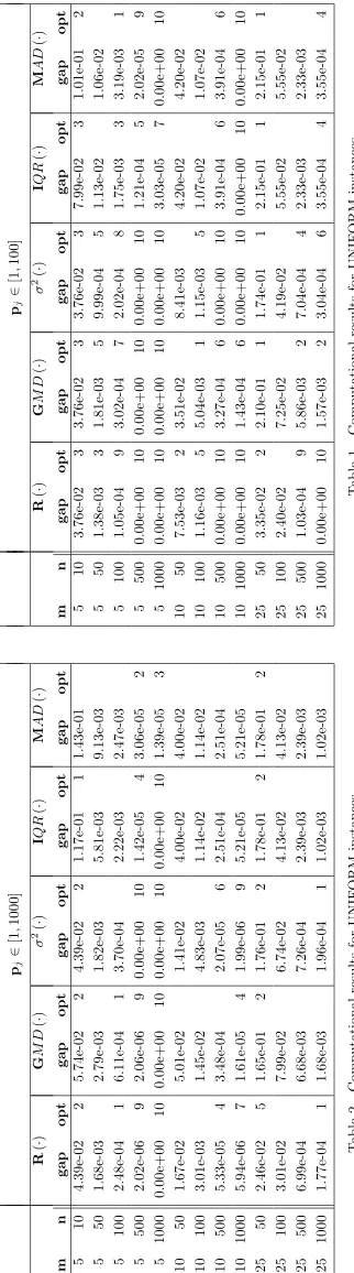
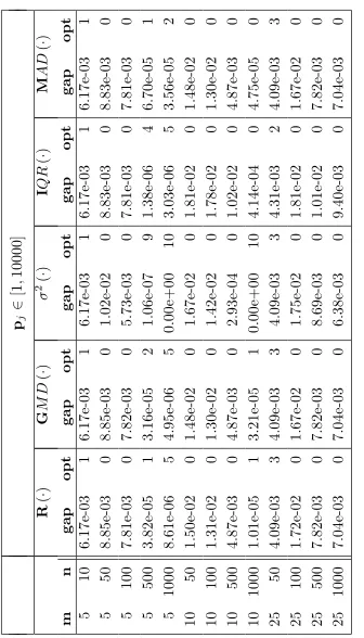
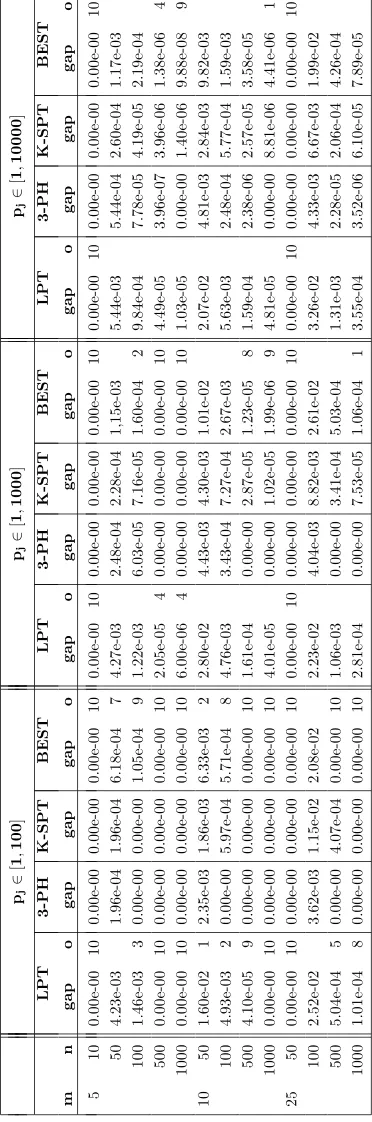
In Tables 1-6 we report the results of the five algorithms. For sake of simplicity, our algorithms are referred with the name of the used measure of spread. In Tables 7 and 8, the columnsLPT,3-PH,K-SPT and BEST describe, respectively, the results of the LPT heuristic, of the algorithm of Fran¸ca et al., of the algorithm of Francioni et al. and of best result between our five variants. Since our results were averaged for groups of ten instances and the ten results can be from different variants, Tables 7 and 8 provide no information on the choice made. On the other hand, no superiority of a specific measure has been observed, so that we are unable to make a choice of the suitable spead measure before the algorithm starts. The number of instances in which the algorithms obtain the makespan equal to the lower bound (which represent the number of instances solved to optimality) is reported in column opt.
Computational Results
Experiments with different measures of spread on these three family of instances have shown that quality of the solutions does not depend strongly on the chosen mea-sure. Moreover, a choice of a particular measure does not lead a significant reduction of the run time. The BIN-PACK instances seem not suitable for a statistical meth-ods approach; in fact, only in the case when the range is used, the obtained solutions were better than the ones provided by LPT. Therefore, we present only the results for the other two families of instances. The results for UNIFORM instances are shown in Table 1-3 and 7 for the three subsets of instances with processing times in [1,100],[1,1000], and [1,10000]. UNIFORM instances are known to be efficiently approached withLPT,3-PHASE
and K-SPT algorithms. LPT usually obtains low gaps, and solves to optimality a fair number of instances, while
3-PHASE and K-SPT offer more accurate results than
LPT. Our algorithms offer significant improvements over
LPT (Table 7); in 15 (resp. in 23) out of 39 cases the av-erage relative error of BEST is comparable with respect to the more accurate3-PHASE (resp. K-SPT). For ex-ample, when the processing times belong to [1,100], the average relative errors ofBEST and3-PHASE are equal in 8 out of 13 cases and when the processing times be-long to [1,10000], the average relative errors of BEST
and K-SPT are equal in 8 out of 13 cases. The results for NONUNIFORM instances are shown in Table 4-6 and 8 for the three subsets of instances with processing times in [1,100], [1,1000], and [1,10000]. These instances are
more difficult than the UNIFORM instances, as greater gaps remain in all of the four algorithms examined. BEST
[image:5.595.346.507.179.757.2]4
Conclusions
In this paper, we proposed nlogn algorithms for solv-ing parallel machine schedulsolv-ing problem to minimize the makespan. These algorithms produce less average rela-tive errors than theLPT algorithm, and, usually, the av-erage relative errors are comparable with those generated by the 3-PHASE and K-SPT improvement heuristics. Our algorithms are based on five different measures of spread, that are techniques commonly employed in statis-tical problems. While the use of each measure possesses some degree of success, no overwhelming superiority of a single measure has been determined.
References
[1] Anderson E.J., Glass C.A., Potts C.N., “Machine scheduling”, Local Search in Combinatorial Opti-mization, Aarts and Lenstra eds., Wiley, New York, pp. 361-414, 1997.
[2] Chen B., Potts C.N., Woeginger G.J., “A review of machine scheduling: Complexity, algorithms and approximability,” Handbook of Combinatorial Opti-mization, Du D.Z. and Pardalos P. eds., Kluwer Aca-demic Publishers, Dordrecht, pp. 21-169, 3/98.
[3] Cheng T., Sin C., “A state of the art review of par-allel machine scheduling research,” European J. of Oper. Res., pp. 271-292, 47/90.
[4] Coffman E.G. Jr., Garey M.R., Johnson D.S., “An application of bin-packing to multiprocessor schedul-ing,”SIAM J. Comput., pp. 1-17, 7/78.
[5] Fran¸ca P.M., Gendrau M., Laporte G., Muller F.M., “A composite heuristic for the identical par-allel machine scheduling problem with minimum makespan objective,”Computers Ops. Res., pp. 205-210, 21(2)/94.
[6] Frangioni A., Scutell`a M.G., Necciari E., “Multi-exchange algorithms for the minimum makespan machine,” Technical Report:99-22, Dipartimento di Matematica, University of Pisa, Italy, 1999.
[7] Frangioni A., Necciari E., Scutell`a M.G., “A multi-exchange neighborhood for minimum makespan ma-chine scheduling problems,” J. Comb. Optim., pp. 195-220, 8/04.
[8] Garey M.R., Johnson D.S., Computers and In-tractability: A guide to the Theory of NP-Completeness, Freeman, San Francisco, CA, 1979.
[9] Graham R.L., “Bounds for certain multiprocessing anomalies,” Bell System Tech. J., pp. 1563-1581, 45/66.
[10] Graham R.L., “Bounds on multiprocessing timing anomalies,” SIAM J. Appl. Math., pp. 416-429, 17/69.
[11] Graham R.L., Lawler E.L., Lenstra J.K., Rinnooy Kan A.H.G., “Optimization and approximation in deterministic sequencing and scheduling. A survey,”
Ann. Discrete Math., pp. 287-326, 5/79.
[12] Gualtieri M.I., Paletta G., Pietramala P., “A new
nlogn algorithm for the identical parallel machine scheduling problem,” Int. J. Contemp. Math. Sci-ences, pp. 25-36, 3(1)/08.
[13] Hochbaum D.S., Shmoys D.B., “Using dual approxi-mation algorithms for scheduling problems: theoret-ical and practtheoret-ical results,”J. Assoc. Comput. Mach., pp. 144–162, 34/87.
[14] Lawler E.L., Lenstra J.K., Rinnooy Kan A.H.G., Shmoys D.B., “Sequencing and scheduling: algo-rithms and complexity in logistics of production and inventory,” Handbooks in Operation Research and Management Science, Elsevier Science Publishers, pp. 445-522, 4/93.
[15] Leung J. (Editor), Handbook of Scheduling: Algo-rithms, Models, and Performance Analysis, Chap-man & Hall/CRC, 2004.
[16] Paletta G., Pietramala P., “A new approximation al-gorithm for the non-preemptive scheduling of inde-pendent jobs on identical parallel processors,”SIAM J. Discrete Math., pp. 313-328, 21/07.
[17] Ullman J.D., “Complexity of sequencing problems,”