Performance Analysis of Comparison between Region Growing, Adaptive Threshold and Watershed Methods for Image Segmentation

T

Performance Analysis of Comparison between

Region Growing, Adaptive Threshold and

Watershed Methods for Image Segmentation

Erwin, Member, IAENG, Saparudin, Member, IAENG, Adam Nevriyanto, Diah Purnamasari

Abstract----Image Segmentation with region growing technique, clustering neighbor’s pixels and similar seed points otherwise adaptive thresholding create fixed blocks and find appropriate threshold values. Using images from Berkeley Segmentation Dataset (BSDS) is BSDS300, including 300 grayscale’s images and 300 color’s images, each of which has 200 training images and 100 testing images. The results are average performance measurement of precision, recall and F-Score each of which has 0.437, 0.665, 0.525 for region growing method and 0.30, 0.525, 0.73 for adaptive thresholding method. While using watershed techniques, we obtained following values: 0.258, 0.488, and 0.333.

Index Terms—Segmentation, Region Growing, Adaptive Thresholding, Watershed.

I INTRODUCTION

here are several methods which is offered in image segmentation based on 1. Intensity Base; 2. Region Base; 3. Others (such as Watershed, Edge, Contour, Color) [1], [2].

Region Growing, a segmentation method based on a region which cluster neighbor’s pixel with has same seed point. For example, if the size of similarity of one or more adjacent pixels is greater than the threshold, these pixels are equivalent. They also will be grouped together [3]. Grouping neighboring pixels continues until there are no same pixels.

However, in this study, the growing region starts from the initial initialization of the region which is obtained from the binary segmentation so that the growing region process becomes faster in time complexity [4].

Adaptive thresholding is a method of Intensity Based segmentation that is considered as the best among other methods. It is also more popular because, in addition to modern or current, thresholding can be easily applied computationally faster in image enhancement [5], [6], [7].

Erwin is with the Computer Engineering Department, University of Sriwijaya, Indralaya, OI 30662 IDN (corresponding author to provide phone: +62 711 589 169; fax: +62 711 580644; email: [email protected]). Saparudin is with the Informatics Engineering Department, University of Sriwijaya, Indralaya, OI 30662 IDN (email: [email protected]).

Adam Nevriyanto is with the Computer Engineering Department, University of Sriwijaya, Indralaya, OI 30662 IDN (email: [email protected]).

Diah Purnamasari is with the Computer Engineering Department, University of Sriwijaya, Indralaya, OI 30662 IDN (email: [email protected])

However, the threshold obtained value is not always appropriate because there are factors from the image of noise, opacity, and ambiguity between classes (image overlapping).

For this reason, this research is proposed with a new methodology that considers the parameters before executing the image. Adaptive thresholding is considered to find optimum results and processing time compared to global thresholding or local thresholding.

II THEORETICAL BASIS

A. Region Growing

Region-based segmentation combines the connectivity steps between pixels to choose whether these pixels belong to the same region or not. In mathematics, region-based segmentation methods can be explained in a systematic way to divide the image I into n, S1, S2, · · ·, Sn, so as to

emphasize the following properties: 1. n

S

I

x





2. Sx which is connected region, x = 1,

2, · · ·, n.

3.

S



S





5. P (Sx∪ Sy) = FALSE for any adjacent regions

Sx and Sy.

P (Si) is a logical predicate which defines points in set Si,

and ∅ is an empty set.

Growing the region method is being started from the pixels. Moreover, it will grow the surrounding area if the resulting region continues to meet the criteria of homogeneity. The bottom-up approach to segmentation, which begins with individual pixels (also called 'seed') and produces a segmented area at the end of the process. The key factors in the growing region are as follows:

a. The Choice of Similarity Criteria; b. The Selection of Seed Points; c. The Definition of a Stopping Rule.

B. Adaptive Thresholding

much better than those obtained with global thresholding. In Matlab, a blkproc function is used for block processing technique.

C. Watershed

The watershed transformation is a morphologic-based transformation function for image segmentation. The use of watershed is recognized as a powerful method because it has the advantage of speed and simplicity [8].

The output of the watershed transformation is a partition of an image consisting of a region (set of pixels connected to a local minimum) and watershed pixels. Typically, the result of the watershed transformation in gradient image without additional process is the over-segmented image. In order to solve this problem we, usually reduce the minimal local value that is filtered using the original image or gradient function (image filtered) or can also do by using a marker. As additional, the problem of over-segmentation can be solved by correcting some images after the process such as combining the neighboring region [9].

III METHODS

A. Region Growing

Region Growing is a procedure how to classify the pixels or sub-region into a larger region based on pre-determined criteria for growth thus it called region growing. It begins with individual pixels (also called 'seed' or seed), the bottom-up approach to segmentation and produces a segmented area at the end of the process.

Fig. 1. (a) pixel ‘seed’; (b) the first iteration; (c) the final iteration

The iteration process to expand the region will take place as long as the outer pixels included into the pixel connectivity of the region are not aligned to the above two criteria again. Regional Growing Algorithm:

Let c(a,b) be the input image

Define a set of regions S1, S2, ..., Sn, each consisting of a single seed pixel

repeat

for x = 1 to n do

for each pixel p at the border of Sx do for all neighbors of p do Let (a,b) be the neighbor’s coordinates

Let Mx be the mean gray level of pixels in Sx if the neighbor is unassigned and

|f(a,b) - Mx| <= Delta then Add neighbor to Rx

Update Mx

end if end for end for

end for

until no more pixels can be assigned to regions.

B. Adaptive Thresholding

The value of T (a, b) is a thresholding that satisfies:

With c (a, b) being the input image as pixel intensity at (a, b) and c (a, b) ∈ [0.1]. If the value of T (a, b) is given equally for all image inputs, this process is called global thresholding, but if the value of T (a, b) is given differently depending on the value of the statistical parameter around (a, b), this process is called Adaptive Thresholding (Local Thresholding).

The general form of Adaptive Thresholding has a threshold value that will adapt to local variances. The usual technique is to create blocks which mean that fixed-size blocks are made in the image and then for each block is searched for the appropriate threshold value. So, the threshold for each block can be various. The Niblack and Sauvola techniques use statistic mean and standard deviation so that it is called the variant method.

Suppose the local mean m (a, b) and the standard deviation δ (a, b) on the block and

)

,

(

)

,

(

)

,

(

a

b

m

a

b

k

a

b

T







called Niblack technique, whereas































(

,

)

1

(

,

)

1

)

,

(

R

b

a

k

b

a

m

b

a

T



called Sauvola technique, whereas

































1

)

,

(

1

)

,

(

1

)

,

(

)

,

(

b

a

b

a

k

b

a

m

b

a

T





called Singh technique [10].

It looks very different from the global thresholding which implements one threshold value for each pixel in the image so that adaptive thresholding is slow the process but it is very able to be adaptep. It aims to spot the illumination and convergent changes either on uniform illumination (uniform) or not [10].

C. Watershed

The Watershed algorithm in [11] represents the watershed transformation applied to the image segmentation. First, define the basic tools for watershed transformation. Second, the transformation was made by implementing the flooding process on the gray-tone image. Then, use the result of the transformation for the segmentation result. The application of watershed transformation is done to the gradient image. The main advantage of using watershed method is to separate region and pixel into the two-step segmentation process.

1. Input training image and test image then convert it into a grayscale image.

2. Using magnitude gradient as the function of segmentation.

3. Marking the foreground object. 4. Counting the background markers.

6. Visualize the results.

D. Dataset and Benchmark Algorithm

The BSDS300 dataset consists of 200 images for training and 100 images for testing. Examples of BSDS300 images are shown in Figure 2. There are 3 sample images and segmentation results from 3 different humans. This dataset is used to build new detection algorithms and benchmarks. Figures 2 and 3 are evaluated by some contour detection in (Fig. 2) and image segmentation in (Fig. 3).

Fig. 2. Berkeley Segmentation Dataset [12], three sample images and segmentation results.

The best approach is based on the order of values F,

recall

precision

recall

precision

F









2

Obtained contour gBp detection [13] is better than algorithm [14], [15], [16], [17], [18], [19], [20], [21], [22], [23], [24], [25], [26]

Fig. 3. Contour Evaluation on BSDS300 [27]

Segmentation evaluation results obtained by gPb-owt-ucm algorithm [28] resulted in a better segmentation region than the method [29], [30], [31], [32], [33], [34], [35], [36].

Fig. 4. Evaluation of Benchmark Algorithm Segmentation on BSDS 300 [27]

IV. EXPERIMENT AND RESULT

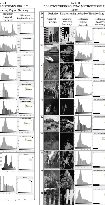
The BSDS300 dataset consisting of 300 grayscale images and 300 image colors (in this paper, we are using image colors). It includes 200 color training images and 100 color testing images (10 figure from each technique are represented in this paper as sample a result) which are using region growing, adaptive threshold and watershed techniques. Table 1, 2, 3 present an example of the original image comparison with the adaptive thresholding, region growing, and watershed histogram techniques of 10 BSDS300 images and the histograms.

In addition to the histogram, Precision-Recall and F-Score value calculations for Adaptive Thresholding and Region Growing techniques are presented in the ROC (Receiver operating characteristic) curve fig. 5-7.

Table I

REGION GROWING METHOD’S RESULT

No

Berkeley’s Dataset using Region Growing

Original Grayscale

Region Growing Boundary

Histogram Original Grayscale

Histogram Region Growing

1

2

3

4

5

6

7

8

*9

*10

* figure no 9 and 10 are image 11th and 12th which replace image 5th and 6th cause both

images take long to respond

Table II

ADAPTIVE THRESHOLDING METHOD’S RESULT C=0.03

N o

Berkeley’ Datasets using Adaptive Thresholding

Original Grayscale

Adaptive

Thresholding

Boundary

Histogram Original Grayscale

Histogram Adaptive

Thresholding

1

2

3

4

5

6

7

8

9

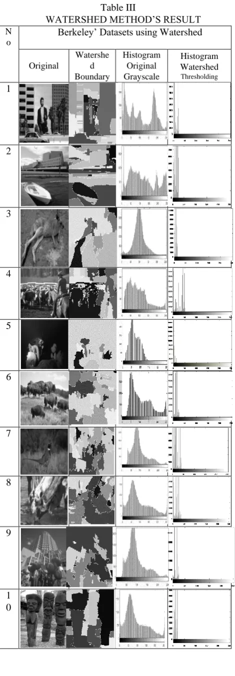
Table III

WATERSHED METHOD’S RESULT

N o

Berkeley’ Datasets using Watershed

Original

Watershe d Boundary

Histogram Original Grayscale

Histogram Watershed

Thresholding

1

2

3

4

5

6

7

8

9

1 0

Fig. 5. ROC Precision’s curve of Region Growing, Adaptive Thresholding, and Watershed

Fig. 6. ROC Recall’s curve of Region Growing, Adaptive Thresholding, and Watershed

Figure 7. ROC F-Score’s curve of Region Growing, Adaptive Thresholding, and Watershed

Table IV

Mean Squared Error is used to compare image before and after segmentation by calculating the mean of the error square between the original image and the image of the processing. The smaller the Mean Squared Error, the closer the fit to segmentation result for determining the best segmentation. The mean-squared error (MSE) between two images f(x,y) and f’(x,y) is:











)

,

(

)

,

(

'

1

MSE

f

x

y

f

x

y

AB

e

Root Mean Squared Error is another quality measurement of an image to measure residual of an image from Mean Squared Error.











)

,

(

)

,

(

'

1

y

x

f

y

x

f

AB

RMSE

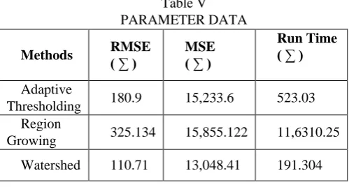
Two of image quality measurement for 300 images from BSDS300 is represented in Table V.

Table V PARAMETER DATA

V ANALYSIS

From the experimental results of using boundary in Matlab, adaptive thresholding segmentation shows segmentation based on light intensity or in other words it cannot be used optimally for the introduction between background and foreground (object) because it does not meet satisfactory result but it is very fast computation processing. While the growing region shows segmentation the surrounding pixel (neighbor) is still inhomogeneity criterion so that its result is enough to do background and foreground introduction. Unfortunately, it is very long computation processing. Images number 5 can not be displayed because of obstacles in computing that takes a very long time. Repetition continues to occur on the identification of neighboring pixels. Watershed shows that segmentation’s result as region and boundary (analogous to ridge line) of image and cannot take the object of image (there’s no clear enough to see foreground and background).

VI CONCLUSION

The research is done by soft computing algorithm which is used is an existing algorithm. It takes the conclusion that the method used adaptive threshold has no faster processing time. Unfortunately, the result must be optimized. The

Region lacks the processing, but we can see better results from adaptive. Watershed has good segmentation and run time but it can not perfectly handle the detail object.

Reference

[1] O. Marques, Practical Image and Video Processing Using MATLAB. New Jersey: A John-Willey & Sons, 2011.

[2] R. C. Gonzalez and R. E. Woods, Digital Image Processing Third Edition. 2008.

[3] C. Wang and G. Lin, “A Study on the Application of Fuzzy Information Seeded Region Growing in Brain MRI Tissue Segmentation,” vol. 2014, 2014.

[4] A. K. Sahoo, G. Kumar, G. Mishra, and R. Misra, “A New Approach for Parallel Region Growing Algorithm in Image Segmentation using MATLAB on GPU Architecture,” pp. 279–283, 2015.

[5] S. Qiang and L. Guoying, “An Edge-Detection Method Based on Adaptive Canny Algorithm and Iterative Segmentation Threshold,” ICCSSE, pp. 64–67, 2016. [6] S. N. Holambe and P. G. Kumbhar, “Comparison

between Otsu ’ s Image Thresholding Technique and Iterative Triclass,” IJCTT, vol. 33, no. 2, 2016.

[7] P. P. Vijay and N. C. Patil, “Gray Scale Image Segmentation using OTSU Thresholding Optimal Approach,” vol. 2, no. 5, pp. 20–24, 2016.

[8] A. Sinha, “A New Approach of Watershed Algorithm using Distance Transform Applied to Image,” Int. J. Innov. Res. Comput. Commun. Eng., vol. 1, no. 2, pp. 185–189, 2013.

[9] Y. Tarabalka, J. Chanussot, and J. A. Benediktsson, “Segmentation and classification of hyperspectral images using watershed transformation,” Pattern Recognit., vol. 43, no. 7, pp. 2367–2379, 2010.

[10] T. R. Singh, S. Roy, O. I. Singh, T. Sinam, and K. M. Singh, “A New Local Adaptive Thresholding Technique in Binarization,” Int. J. Comput. Sci. Issues, vol. 8, no. 6, pp. 271–277, 2012.

[11] S. Saini and K. Arora, “A Study Analysis on the Different Image Segmentation,” Int. J. Inf. Comput. Technol., vol. 4, no. 14, pp. 1445–1452, 2014.

[12] D. Martin, C. Fowlkes, D. Tal, and J. Malik, “A Database of Human Segmented Natural Images and its Application to Evaluating Segmentation Algorithms and Measuring Ecological Statistics,” ICCV, vol. 2, pp. 416--423, 2001.

[13] M. Maire, P. Arbel, C. Fowlkes, and J. Malik, “Using Contours to Detect and Localize Junctions in Natural Images,” CVPR, 2008.

[14] L. G. Roberts, Machine perception of three-dimensional solids. 1965.

[15] R. O. Duda, P. E. Hart, and J. Wiley, PATTERN

CLASSIFICATION AND SCENE ANALYSIS. 1973.

[16] J. M. S. Prewitt, “Pattern Classification and Scene Analysis.” 1970.

[17] B. Y. D. Marr, “Theory of edge detection,” vol. 217, pp. 187–217, 1980.

[18] J. Canny, “A Computational Approach to Edge Detection,” no. 6, 1986.

[19] D. R. Martin, C. C. Fowlkes, and J. Malik, “Learning to Detect Natural Image Boundaries Using Local Brightness , Color , and Texture Cues,” vol. 26, no. 1, pp. 1–20, 2004.

Methods RMSE ( ∑ ) MSE ( ∑ )

Run Time ( ∑ )

Adaptive

Thresholding 180.9 15,233.6 523.03 Region

Growing 325.134 15,855.122 11,6310.25

[20] J. Mairal, M. Leordeanu, and F. Bach, “Discriminative Sparse Image Models for Class-Specific Edge Detection and Image Interpretation,” ECCV, pp. 1–14, 2008. [21] P. Dollar, Z. Tu, and S. Belongie, “Supervised Learning

of Edges and Object Boundaries,” CVPR, 2006.

[22] X. Ren, C. C. Fowlkes, and J. Malik, “Scale-Invariant Contour Completion using Conditional Random Fields,”

ICCV, 2005.

[23] Q. Zhu, G. Song, and J. Shi, “Untangling Cycles for Contour Grouping,” ICCV, no. c, pp. 1–8, 2007. [24] P. Felzenszwalb and D. Mcallester, “A Min-Cover

Approach for Finding Salient Curves,” POCV, 2006. [25] X. Ren, “Multi-Scale Improves Boundary Detection in

Natural Images,” ECCV, 2008.

[26] P. Perona, J. Malikt, and U. Padova, “Detecting and localizing edges composed of steps , peaks and roofs *,” vol. 171, 1990.

[27] P. Arbel, M. Maire, C. Fowlkes, and J. Malik, “Contour Detection and Hierarchical Image Segmentation,” IEEE TPAMI, vol. 33, no. 5, pp. 898–916, 2011.

[28] P. Arbel, M. Maire, C. Fowlkes, and J. Malik, “From Contours to Regions : An Empirical Evaluation ∗,”

CVPR, 2009.

[29] P. Arbelaez, “Boundary Extraction in Natural Images Using Ultrametric Contour Maps,” POCV, 2006. [30] A. Y. Yang, J. Wright, Y. Ma, and S. S. Sastry,

“Unsupervised segmentation of natural images via lossy data compression,” vol. 110, pp. 212–225, 2008. [31] M. Donoser, M. Urschler, M. Hirzer, and H. Bischof,

“Saliency Driven Total Variation Segmentation,” ICCV, 2009.

[32] L. Bertelli, S. Member, and B. Sumengen, “A Variational Framework for Multi-Region Pairwise Similarity-based Image Segmentation,” PAMI, no. 1, pp. 1–15, 2008.

[33] E. Sharon, M. Galun, D. Sharon, R. Basri, and A. Brandt, “Hierarchy and adaptivity in segmenting visual scenes,” vol. 442, no. August, pp. 2–5, 2006.

[34] P. F. Felzenszwalb and D. P. Huttenlocher, “Efficient Graph-Based Image Segmentation,” IJCV, pp. 1–26, 2004.

[35] T. Cour, F. Benezit, and J. Shi, “Spectral Segmentation with Multiscale Graph Decomposition,” CVPR, 2005. [36] D. Comaniciu, P. Meer, and S. Member, “Mean Shift :