Dissonance Metrics: Applications for Microtuning

Measuring Roughness: considerations for the

microtonalist

Richard Duckworth

Contexts

๏

exploration of xenharmonic scales and the holistic inclusion of factors

such as interface and timbre as factors

๏

...and also assess historical uses of tunings and perceptions of

dissonance - as these can differ from our own

๏

The use of the scale leads to the evolution of a music theory

Roughness

๏

Roughness one of the auditory attributes along with Pitch, Timbre

and Loudness.

๏

as distinct from dissonance - culturally loaded and context dependent

๏

dissonance = ‘sensory dissonance’

๏

first research without cultural bias: Helmholtz 1885

๏

little research carried out in the area until the 1960’s (with the

exception of von Békésy’s work in the 1930-40’s)

๏

von Békésy, (1960); Terhardt, (1974); Plomp & Levelt, (1965);

Kameoka & Kuriyagawa, (1969); Hutchinson & Knopoff, (1978);

Consonance & Dissonance

๏

That certain conditions cause the ear to be ’thrown into turmoil’ has

been observed throughout the ages.

๏

psychoacoustics research explains these physiological and perceptual

phenomena.

๏

tones which lie closely together in frequency exhibit a phenomenon

known as beating as they cycle in and out of phase with one another

rapidly.

๏

this swift beating (fluttering) is perceived as roughness and persists

until the tones are separated by a distance known as the critical band.

๏

when a number of tones and or their partials lie within the same

Critical Bands

๏

Fletcher’s ‘Auditory Patterns’,

(1940) - the graphics

highlight areas of excitation on the basilar membrane

๏

the existence of CBs was

confirmed by the

phenomenon of masking: a noise signal concealed a sine

wave from the subject.

However, when the the sine

wave was swept up or down

in pitch, it it would reappear

- confirming the existence of

place-specific areas of

sensitivity.

Critical Bands

๏

The width of the CBs was

later mapped by Zwicker,

‘Subdivision of the Audible Frequency Range

(Frequenzgruppen)’, (1961)

๏

and presented as a table

Plomp & Levelt

๏

First to tie concept of roughness perception to the parameters of the

Critical Band*

๏

found that maximum roughness point occurs at 1/4 width of the CB

๏

and that the curve is wider for lower frequencies

Terhardt

๏

attributes the sensation of roughness directly to temporal fluctuations

in amplitude when they appear within the ‘spectral regions’ known as

critical bands (CBs).

๏

the roughness created across all of the CBs is summed to give an

overall roughness effect

๏

confirming the assumption that, for a pair of timbres, adjacent

partials of each timbre that lie within the same CB will contribute to

the overall sensation of roughness.

๏

Terhardt mentions phase but does not present any process for dealing

Parncutt

๏

Terhardt’s ideas (tonalness, virtual pitch) were extended by Parncutt.

๏

applied them to common practice music & 12 tet composition

๏

implemented an extended version of Hutchinson & Knopoff’s

Vassilakis

๏

pan-musical interdisciplinary dissertation (2005) inclusive of non

-Western music

๏

clarifies the confusion surrounding amplitude fluctuation and

amplitude modulation depth

๏

highlights importance of roughness as an integral sonic attribute of

many types of music

๏

revises models estimating to roughness of complex tones with a

Bohlen Pierce

๏

non-octave scale with 13 steps

๏

repeats every 12th

๏

Just Intonation and Equal Tempered versions

๏

None of the BP scales sit well on the physical key arrangement of the

12-TET keyboard

๏

so following from Elaine Walker (and from Heinz Bohlen) , a

Bohlen Pierce Just Intonation

๏

BP Just Intonation (JI) chromatic

1/1, 27/25, 25/21, 9/7, 7/5, 75/49, 5/3, 9/5, 49/25, 15/7, 7/3, 63/25, 25/9, 3/1

๏

BP JI diatonic: ‘Lambda Mode’

1/1, 25/21, 9/7, 7/5, 5/3, 9/5, 15/7, 7/3, 25/9, 3/1

C D E F G H J A B C’

๏

The keyboard provides a ‘front-end’ for an

additive synthesis instrument implemented in

Pure Data. The partials have high resolution

frequency and amplitude controls, and there

are individual envelopes on each partial.

๏

Diatonic BP notes mapped to white keys, and

the ratios corresponding to the chromatic notes

are mapped to the reconfigured black keys.

๏

Only parts of the MIDI protocol are used (e.g.,

velocity). The frequency values assigned to the

keys are not used; instead each unique MIDI

note ID is re-assigned to trigger scale maps

created within the pd patch itself.

๏

The synthesizer allows the user to select either

ET or JI BP scales

BP JI chromatic scale mapped out as a set of message boxes

in pd

These are then sent sequentially through an

expression for the

calculation of the ratios...

... and mapped out on an

array to provide scale ratios to be applied to a base

Timbres that complement B

-

P

๏

B-P practitioners have traditionally chosen timbres consisting of odd

integer multiples of the fundamental.

๏

Preliminary tests with triangle and square waves confirmed the

suitability of these types

๏

Sethares presents a useful way of constructing a spectrum for a given

scale

๏

‘Symbolic Computation of Spectra’ is a technique for selecting spectral

components with the goal of maximising the number of co-incident

partials.

๏

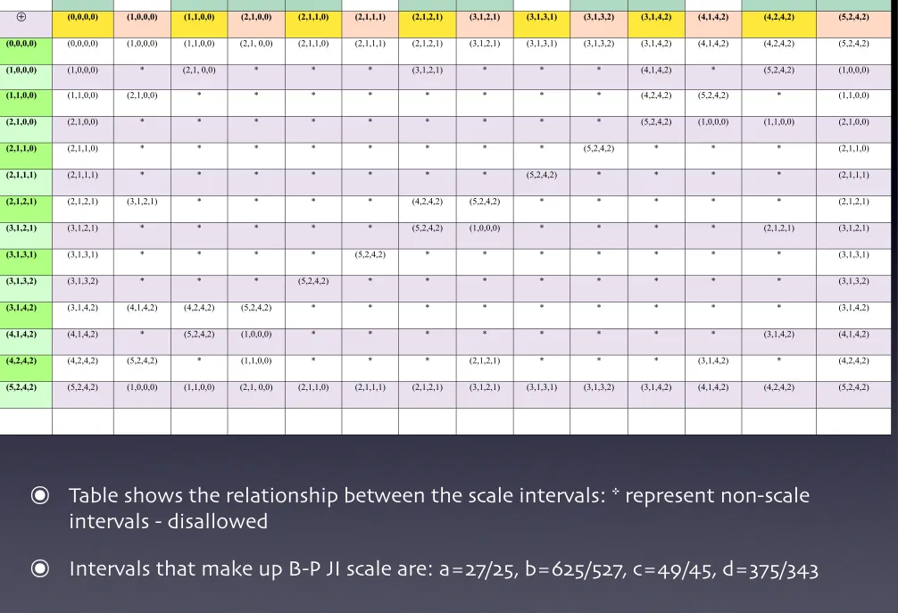
This is accomplished by ensuring that the ratios between the partials

1/1 27/25 25/21 9/7 7/5 75/49 5/3 9/5 49/25 15/7 7/3 63/25 25/9 3/1

⊕ (0,0,0,0) (1,0,0,0) (1,1,0,0) (2,1,0,0) (2,1,1,0) (2,1,1,1) (2,1,2,1) (3,1,2,1) (3,1,3,1) (3,1,3,2) (3,1,4,2) (4,1,4,2) (4,2,4,2) (5,2,4,2) (0,0,0,0) (0,0,0,0) (1,0,0,0) (1,1,0,0) (2,1, 0,0) (2,1,1,0) (2,1,1,1) (2,1,2,1) (3,1,2,1) (3,1,3,1) (3,1,3,2) (3,1,4,2) (4,1,4,2) (4,2,4,2) (5,2,4,2)

(1,0,0,0) (1,0,0,0) * (2,1, 0,0) * * * (3,1,2,1) * * * (4,1,4,2) * (5,2,4,2) (1,0,0,0)

(1,1,0,0) (1,1,0,0) (2,1,0,0) * * * * * * * * (4,2,4,2) (5,2,4,2) * (1,1,0,0)

(2,1,0,0) (2,1,0,0) * * * * * * * * * (5,2,4,2) (1,0,0,0) (1,1,0,0) (2,1,0,0)

(2,1,1,0) (2,1,1,0) * * * * * * * * (5,2,4,2) * * * (2,1,1,0)

(2,1,1,1) (2,1,1,1) * * * * * * * (5,2,4,2) * * * * (2,1,1,1)

(2,1,2,1) (2,1,2,1) (3,1,2,1) * * * * (4,2,4,2) (5,2,4,2) * * * * * (2,1,2,1)

(3,1,2,1) (3,1,2,1) * * * * * (5,2,4,2) (1,0,0,0) * * * * (2,1,2,1) (3,1,2,1)

(3,1,3,1) (3,1,3,1) * * * * (5,2,4,2) * * * * * * * (3,1,3,1)

(3,1,3,2) (3,1,3,2) * * * (5,2,4,2) * * * * * * * * (3,1,3,2)

(3,1,4,2) (3,1,4,2) (4,1,4,2) (4,2,4,2) (5,2,4,2) * * * * * * * * * (3,1,4,2)

(4,1,4,2) (4,1,4,2) * (5,2,4,2) (1,0,0,0) * * * * * * * * (3,1,4,2) (4,1,4,2)

(4,2,4,2) (4,2,4,2) (5,2,4,2) * (1,1,0,0) * * * (2,1,2,1) * * * (3,1,4,2) * (4,2,4,2)

(5,2,4,2) (5,2,4,2) (1,0,0,0) (1,1,0,0) (2,1, 0,0) (2,1,1,0) (2,1,1,1) (2,1,2,1) (3,1,2,1) (3,1,3,1) (3,1,3,2) (3,1,4,2) (4,1,4,2) (4,2,4,2) (5,2,4,2)

๏

Table shows the relationship between the scale intervals: * represent non-scale

intervals - disallowed

[image:19.1024.18.1024.64.751.2]

๏

Spectrum t(i) constructed by consulting O-plus table and selecting likely candidates.

Then partials are tested against each other: f(i)/f(j) = scale step. In this case, not all

of the ratios between partials are scale steps, so this timbre is only partly related to

the B-P scale

i 1 2 3 4 5 6 7 k

t(i) (0,0,0,0) (5,2,4,2) (9,4,8,4) (12,5,8,4) (13,5,10,5) (13,5,12,6) (14,5,12,6) s(i) (0,0,0,0) (0,0,0,0) (4,2,4,2) (2,1,0,0) (3,1,2,1) (3,1,4,2) (4.1.4.2)

r (i,k) (5,2,4,2) (4,2,4,2) * * * (1,0,0,0) ₁ (4,2,4,2) (2,1,0,0) * * * 2

(2,1,0,0) (3,1,2,1) (4,1,4,2) * 3

(3,1,2,1) (3,1,4,2) _{* 4}

(3,1,4,2) (4.1.4.2) 5

Roughness curves

๏

in contrast to the JI advocates, tuning creators who manipulate

timbral components for the purposes of achieving coherence of

partials with scales that would not work with acoustic timbres occupy

a space of their own in contemporary tuning studies.

๏

utilising the flexibility granted by digital synthesis and control

systems, researchers are able to create scales that would be bereft of

consonance if used with timbres containing ‘partial placements’

usually associated with traditional instruments.

๏

The reverse process also holds true - a unique scale can be derived

๏

dissonance curve of spectrum of waterphone sample drawn using Moore and Glasberg’s formula for the calculation of CB

๏

the pd patch models the way the ear perceives dissonance by reacting

each partial together and testing for roughness. The amplitude of the

partials is taken into account, as is register, by including a critical band

model.

๏

the result is a curve which clearly shows the ‘dissonance minima’

๏

it is at these points that the scale steps are fixed

๏

In this case the next most consonant interval, after unison (8ve), is a

type of tritone - this timbre supports the tritone as a consonant

Dissonance curve

๏

To port these minima over so that they form a meaningful scale it is

necessary to get the values out of the table and into a scale implementation device

๏

this time Kontakt was used: both to host the samples and to

implement the scales. It has the disadvantage of being 8ve based.

๏

the values from 0-400 are easily readable from the curve x-axis

๏

these are *3 to give 1200 - so that it now fits neatly across a 12 TET

span

Curve values for minima points

*3

(1200 cents)

Assigned note - Kontakt

0 0 C (base note)

46 138 Db

77 231 D

130 390 E

196 570 Gb

222 666 G

329 987 Bb

Rich Duckworth NUI Maynooth

๏

Moore & Glasberg’s CB equation. Fcb = critical bandwidth,

Fm = mean frequency