A simple two module problem to exemplify building block assembly under crossover

A Simple Two-Module Problem to Exemplify

Building-Block Assembly Under Crossover

Richard A. Watson

Harvard University, Organismic and Evolutionary Biology, Cambridge, MA 02138, USA

[email protected]

Abstract. Theoretically and empirically it is clear that a genetic algorithm with crossover will outperform a genetic algorithm without crossover in some fitness landscapes, and vice versa in other landscapes. Despite an extensive literature on the subject, and recent proofs of a principled distinction in the abilities of crossover and non-crossover algorithms for a particular theoretical landscape, building general intuitions about when and why crossover performs well when it does is a different matter. In particular, the proposal that crossover might en-able the assembly of good building-blocks has been difficult to verify despite many attempts at idealized building-block landscapes. Here we show the first example of a two-module problem that shows a principled advantage for cross-over. This allows us to understand building-block assembly under crossover quite straightforwardly and build intuition about more general landscape classes favoring crossover or disfavoring it.

1 Introduction

In this paper we introduce a simple abstract fitness landscape that shows a princi-pled advantage for crossover. More importantly, this landscape is the first to show a case where building-block assembly of just two building-blocks is possible under crossover but not possible for a mutation-only method. This example enables us to see a general principle where parallel discovery of high-fitness schemata is easy but sequential discovery of the same schemata is difficult – thus preventing a hill-climber-like process from succeeding. This landscape includes strong fitness interac-tions within blocks (when compared to the interacinterac-tions between building-blocks) which corresponds well with the intuitions proposed by the building-block hypothesis. It should be noted however, that the parallel discovery of high-fitness schemata requires suitable methods for maintaining population diversity. In [13] Jansen systematically removed duplicate genotypes, and our prior work [16] used deterministic crowding [17] – both methods assume that genotypic diversity was meaningful for maintaining diversity. In this paper we use a simple multi-deme island model [18] to maintain diversity.

The following sections describe our model landscape, algorithms, and simulation results.

2 A Two-Module Fitness Landscape

We assume a genotype is a vector of 2n binary variables, G=<g1,g2,…,g2n>, and

define the fitness of a genotype, f(G), as follows:

f(G)=R(i,j)(2i+2j) (1)

where i is the number of 1s in the first half of the genotype, (i.e. {g1,g2,…,gn}), and j

is the number of 1s in the second half of the genotype (i.e. {gn+1,gn+2,…,g2n}), and R(i,j)

returns a value drawn uniformly in the range (0.5,1] for each pair i and j – (these

values may be re-drawn to create different instances of the problem, but remain fixed throughout a given simulation run). This function can be interpreted as a function

over the number of ‘good mutations’ in each of two genes each consisting of n

nu-cleotide sites. The ‘good mutations’ being the 1s at each site, and the two genes

corre-sponding to the left and right halves of the genotype (Fig. 1.).

Fig. 1. A genotype is divided into two genes, left and right, and the number of 1s in each half is counted.

The good ‘alleles’ for each gene then are the all-1s configurations for the

corre-sponding half of the genotype. The terms 2iand 2j simply create a landscape that has

very strong synergy between sites within genes and additive fitness effects for sites in

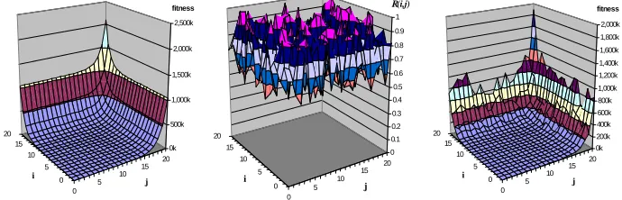
different genes. The effect of these two terms is depicted in Fig. 2. (left). R(i,j) then

0 0 0 1 1 1 1 0 0 1 0 1 1 0 1 0 0 0 1 0

defines a fixed array of ‘noise’ (Fig. 2. center). The product of these components, as defined by Equation 1, creates the landscape depicted in Fig. 2. (right).

0 5 10 15 20 0 5 10 15 20 0 0.1 0.2 0.3 0.4 0.5 0.6 0.7 0.8 0.9 1 R(i,j) j i 0 5 10 15 20 0 5 10 15 20 0k 500k 1,000k 1,500k 2,000k 2,500k fitness j i 0 5 10 15 20 0 5 10 15 20 0k 200k 400k 600k 800k 1,000k 1,200k 1,400k 1,600k 1,800k 2,000k fitness j i

Fig. 2. Landscape defined by Eq. 1 and its component terms. Left) 2i₊₂j_{. Center) R}

(i,j). Right)

R(i,j)(2 i

+2j).

2.1 Motivations

The motivation for this function is as follows. It defines two obvious building-blocks – the all-1 alleles of each gene – where each building-block is easy to find starting from a random genotype. This is true because 1-mutations are strongly rewarded within each gene and these fitness contributions are strong enough to overcome the random noise in the landscape. However, having found a good allele for one gene it becomes difficult to find the good allele for the other gene as the noise in the fitness function prevents progress along the ridges. This prevents an optimization process

from accumulating the good alleles for the two genes sequentially. A hill-climbing

process, for example, will become stuck on some local peak on either of the two

ridges shown in Fig. 2 (right) (although the i=j diagonal is monotonically increasing

in fitness, the stronger fitness gradients pull the search process away from the

diago-nal toward the ridges). In contrast, a process that can find good alleles in parallel

would be able to find both alleles easily – and subsequent crossover between an indi-vidual having the good allele for gene 1 with an indiindi-vidual having the good allele for gene 2 may create a single individual that has the good alleles for both genes. Such a cross creates a new individual at the intersection of these two ridges, and this inter-section necessarily corresponds to the highest fitness genotypes because this is where

both additive components, i.e. 2i and 2j, are maximized.

inter-estingly different from variation from spontaneous point mutations, as we will dis-cuss.

2 Algorithm Models

In the following simulations we use a genetic algorithm [1] with and without cross-over, or sexual recombination, to illustrate the different search behaviors afforded by crossover and non-crossover mechanisms. To afford a meaningful comparison we will use a subdivided population in both cases – this will show that increased diver-sity alone is not sufficient for success in this landscape. We use island migration [18] between sub-populations – i.e. equal probability of migration between all subpopula-tions symmetrically. Each sub-population creates a new generation by fitness propor-tionate selection (with replacement), [18],[19],[1]. The crossover method uses one-point crossover, where for each pair of parents an inter-local position is chosen at random and the sites to the left of this position are copied from parent one, and the sites to the right are copied from parent two. In both the crossover and non-crossover methods, new individuals are subject to a small amount of point mutation – assigning a new random allele at each site with a small probability. For our purposes here we are not interested in the complications arising from loss of fit genotypes through ge-netic drift. Accordingly we use a small amount of elitism – i.e. we retain one copy of the fittest individual in each deme from the prior generation without modification. This is not essential to see the effect shown – it is merely used so that we know that the effect applies even when populations have no problem retaining high-fitness genotypes under mutation and stochastic selection, even when the populations are small. The use of elitism ensures that each deme performs at least as well as a muta-tion hill-climber (with a small overhead for the size of the deme). In fact, in the simu-lations that follow each deme behaves very much like a hill-climber, having a highly converged population, and algorithmically, could logically be replaced by a hill-climber. Crossover between individuals in the same deme is therefore more or less redundant, and it is crossover between a migrant and the individuals of another deme that does the interesting variation in the search process.

3 Simulations and Results

We used a total population of 400 individuals, subdivided into 20 demes of 20 indi-viduals each. Migration between demes was such that one individual in each new generation in each deme was a migrant from some other randomly selected deme.

Each individual in each deme is initialized to a random binary string of length 2n.

Mutation was applied at a rate of 1/2n per site. In the crossover method, one-point

crossover was applied to all reproduction events. In the following experiments we

varied n, the number of sites in each gene, and recorded the number of generations

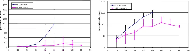
In Fig. 3 we see that the time for the crossover method to find the fittest genotype

remains low even for large n. Whereas in contrast, the time for the non-crossover

method increases dramatically with n. Runs that fail to find the peak in the evaluation

limit of 2000 generations are not plotted. In Figure 3 (right) we can see that this

in-crease for the non-crossover method is approximately exponential in n, as indicated

by an approximately straight line on a log scale. (The last point on this curve falls off from an exponential increase – this is possibly due to the fact that some runs do not

succeed in 2000 generations with n=50 – the average of those runs that do succeed

thus appears low since it does not include the evaluations used by runs that failed.)

0 200 400 600 800 1000 1200 1400 1600 1800 2000

0 10 20 30 40 50 60 70 80 90

n gene ra tions to pea k no crossover with crossover 0 200 400 600 800 1000 1200 1400 1600 1800 2000

0 10 20 30 40 50 60 70 80 90

n gene ra tions to pea k no crossover with crossover 1 10 100 1000 10000

0 10 20 30 40 50 60 70 80 90

n g e ne rat ion s t o pe ak no crossover with crossover 1 10 100 1000 10000

0 10 20 30 40 50 60 70 80 90

n g e ne rat ion s t o pe ak no crossover with crossover

Fig. 3. Left) Results of simulations for a subdivided-population genetic algorithm, on the fit-ness function defined in Equation 1, with and without crossover. Each point is the mean time to reach the peak of the fitness function averaged over 30 independent runs. Error bars show +/- one standard deviation. Right) as (left) but shown with log scale on vertical axis.

3.1 Mutation Rates, Crossover Rates, and the Genetic Map.

We should not be so much interested in the quantitative times shown in these simula-tion results – they should be taken merely as an illustrasimula-tion of the qualitative effect that is quite expected from the design of the fitness function. Simulations using larger and smaller numbers of sub-populations and larger and smaller numbers of individu-als per sub-populations showed qualitatively similar results. However, if the number of populations was reduced too much then occasionally all demes would happen to find the high-fitness allele of the same gene – subsequent crossing of migrants among these demes thus had no significant effect and the run would fail. Similarly, if the migration rate between demes is increased too far then fit migrants from one deme will invade other demes and cause the population as a whole to converge before al-leles for both genes and successful crossing can occur.

expected distance of a local optimum to the global optimum increases linearly with n, a method relying on fortuitous mutations will still show the exponential increase in

time to the peak observed above for increasing n. Exploratory simulations with larger

mutation rates agree with this reasoning – for n=60 we found no mutation rate that

could find the peak of the function in the evaluation limit of 2000 generations. Note that the progress of a mutation-only method would be even more difficult if we were not using elitism because a higher mutation rate would decrease the ability of a popu-lation to retain high-fitness genotypes when discovered.

Variation in the rate of crossover or number of crossover points should also be considered. Fig. 5. illustrates the crossover of two individuals, P1 and P2, which have good alleles for complementary genes. The resultant offspring, C, must have the same bits as both parents at loci where the bits in the parents agree (before mutation is applied). Under uniform crossover, [20], where loci are taken from either parent with equal probability independently, the loci where the parents disagree may take either 0

or 1 with 0.5 probability, as indicated by “?”s in Fig. 4. The chances of a recombinant

offspring produced by uniform crossover having all-1s therefore decreases

exponen-tially with the number of loci where the parents disagree. Since this increases

ap-proximately linearly with n, the expected time for a successful cross under uniform

crossover increases approximately exponentially with n.

P1 11111111110101001010 P2 00010100101111111111 C ???1?1??1??1?1??1?1?

Fig. 4. Crossover of two individuals, P1 and P2, produces some offspring genotype C.

This can also be understood geometrically. Fig. 5. shows the state of all the demes in the subdivided population for no crossover, one-point crossover, and uniform crossover. We see that all demes are clustered close to one ridge or the other in the left frame (mutation only, no crossover). In Fig. 5. (center) using one-point crossover we see that in addition to some demes scattered along the ridges, some demes have recombinant individuals that are at the top-right corner of the frame – corresponding to the fittest genotypes. In contrast, Fig. 5. (right) using uniform crossover shows a few demes that have recombinants produced by crossing individuals from one ridge with individuals from the other ridge, but these recombinant genotypes are very unlikely to be at the peak. Although a cross that produces the all-1s genotype is pos-sible under uniform crossover, this is only one of a very large number of pospos-sible recombinants, increasing exponentially with the number of loci where the parents disagree. Accordingly, recombinants that land on the peak are exponentially unlikely, and most recombinants land somewhere on the straight line between the two demes of

the parents in the ixj space. Fig. 5. (right) shows a couple of demes having

approxi-mately half the good mutations from P1 and half the good mutations from P2. These geometric considerations illustrate well the principles explained in [21] and [22] with respect to the distribution of offspring under crossover.

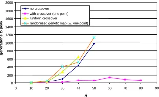
of a building-block as Holland [1] conceived it – i.e. a schema of above average fit-ness and short defining length (distance between first and last loci of the schema). Simulation runs with a randomized genetic map – i.e. where the subsets of loci used

to define i and j are random disjoint sets of n sites each, rather than the left and right

halves of the genotype – show performance similar to that of the non-crossover method (Fig. 6.). Similarly, simulations using uniform crossover also show perform-ance similar to that of the non-crossover method, as expected (Fig. 6.).

o o o o o o o o o o o o o o o

o o o o o o o o o o o o o o o o o o

o o o o o o o o o o o o o o o o

Fig. 5. Snap-shot of the demes at around 200 generations for three different crossover models. In each frame, the horizontal axis is the number of 1s in the first gene and the vertical axis is the number of 1s in the second gene – i.e. these axes correspond to i and j in Equation 1, and the horizontal plane used in Fig. 2. Each small circle within each frame indicates the genotypes of a deme – specifically, it shows the i,j pair for the fittest individual in that deme. Left) A run with no crossover. Center) A run with one-point crossover. Right) A run with uniform cross-over. 0 200 400 600 800 1000 1200 1400 1600 1800 2000

0 10 20 30 40 50 60 70 80 90

n g e ne ra ti ons t o pe a k no crossover with crossover (one-point) Uniform crossover randomized genetic map (w. one-point)

0 200 400 600 800 1000 1200 1400 1600 1800 2000

0 10 20 30 40 50 60 70 80 90

n g e ne ra ti ons t o pe a k no crossover with crossover (one-point) Uniform crossover randomized genetic map (w. one-point)

Fig. 6. Simulation results for control experiments using uniform crossover and also for one-point crossover but with a randomized genetic map. Curves for “no crossover” and “with crossover (one-point)” are as per Fig. 4. (left) for comparison.

4 Discussion

kind of building-block assembly is straightforward it is worth discussing why it has been difficult to illustrate in previous simple building-block models.

The Royal Road functions [24], for example, like other concatenated building-block functions [25], have the property that the evolvability of each building-building-block is insensitive to the configuration of bits in other block partitions. Specifically, the fit-ness rank-order of schemata in each partition is independent of other partitions… Considering a hill-climbing process to start with, we may discard fitness-scaling is-sues. For a hill-climber then, the evolvability of a high-fitness genotype is controlled by the fitness rank-order of different genotypes. This controls the number of muta-tional pathways from a given genotype to another given genotype of higher fitness, for example. When partitions are separable, in this sense of independent fitness rank-orders for schemata within the partition, it means that: If it is possible for a

hill-climber to find a high-fitness schema in some genetic background then it is possible

for it to find that high-fitness schema in any genetic background. Accordingly, the

evolvability of high-fitness schemata in each partition is independent of the configu-rations in other partitions. This means that there is nothing to prevent an optimization process from accumulating beneficial schemata sequentially. Accordingly, if a hill-climber can find high-fitness schemata in each partition, it can find the fittest geno-types (having high-fitness schemata in all partitions). In such naïve building-block functions the action of crossover is thus not required to find high-fitness genotypes.

In contrast, in the function we have described here, and in prior functions such as Jansen’s ‘gap function’, [13], and Watson’s ‘HIFF’ function [14], the evolvability of a fit schema in one partition is strongly dependent on the genetic background. Spe-cifically, in [13] the fittest genotype consists only of 1-alleles, and from a random (low-fitness) genotype, increasing the number of 1-alleles is easy because they are individually rewarded. However, when the number of 1-alleles on background loci is high, increasing the number of 1-alleles on subsequent loci is not rewarded. Accord-ingly, it is not possible for a hill-climbing algorithm to accumulate all the 1-alleles sequentially. In [14] the situation is a little different. Here the fittest configuration for

one building-block is equally either all-1s or all-0s given a random genetic

back-ground at a neighboring block. However, when the neighboring block is well-optimized, one of these fit configurations becomes fitter than the other depending on how the neighboring block was solved. This can still be understood as a function that prevents sequential accumulation of good schemata by using epistasis such that the discovery of the fittest schemata becomes more difficult as other partitions become well-optimized.

The landscape introduced in this paper works via this principle but illustrates the idea straightforwardly using two obvious building-blocks. It is the random noise

component, R(i,j), that prevents the sequential evolution of good schemata: When

neither gene is well-optimized, the fitness contributions of 1s in either gene are strong

enough to overcome these random fluctuations in the landscape; But when one of the

genes is already optimized, the fitness contributions of 1s in the other gene are

indi-vidually relatively insignificant compared to the random fluctuations. This is easily

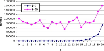
seen using the two cross-sections of the fitness landscape shown in Fig. 7. When i=0

search towards the all-1s allele (although they may be low in magnitude sometimes).

In contrast, when i=20 increasing j is not reliably correlated with increasing fitness.

It should be clear that the possibility of combining good building-blocks together is available in prior simple building-block landscapes such as [24] and [25]. How-ever, this operation of crossover is not necessary for finding fit genotypes when it is possible to accumulate building-blocks sequentially. This is the observation provided by Jones [8] when he applied macro-mutation hill-climbers to concatenated sub-function problems. It is the relatively subtle manner in which the evolvability of a building-block changes with genetic background that is important in the design of the function we have shown here. Specifically, the salient properties of this function are that there are relatively independent fitness contributions provided for each of the building-blocks (with epistasis and the genetic map in good correspondence), but additionally, the other important feature is that the discovery of good alleles for these partitions becomes more difficult as more partitions become well-optimized. This seems not unreasonable in some circumstances – for example, as the number of func-tioning modules increases, the number of dependencies affecting the evolution of subsequent modules also increases, thus making them less evolvable – but it is not our intent here to argue for this in general.

0 200000 400000 600000 800000 1000000 1200000 1400000 1600000 1800000

0 1 2 3 4 5 6 7 8 9 10 11 12 13 14 15 16 17 18 19 20

j

fi

tn

e

s

s

i=0 i=20

Fig. 7. Two cross sections through the landscape defined by Equation 1. One curve shows the fitness for different values of j when i=0, the other for different values of j when i=20.

4 Conclusions

In this paper we have provided a simple two-module building-block function that illustrates a principled advantage for crossover. It is deliberately designed to be easy for crossover whilst being difficult for a hill-climber, in a manner that makes the simulations easy to predict and understand. In particular, this model exemplifies the advantage of crossover from the assembly of individually fit building-blocks as per the building-block hypothesis [1],[9],[10],[11]. However, an important characteristic of this model is that the sequential discovery of fit building-blocks is prevented – in this case, by arbitrary epistatic noise that becomes more important as other genes are optimized. This characteristic is analogous to some properties of prior models, [13],[14], but notably, it is not part of the original intuition of the building-block hypothesis.

cross-over. It also provides a simple illustration of the dependencies of this advantage on the properties of epistatic structure and the genetic map. It is notable that the simple form of modularity used here (Fig.1), where genes are constituted by a large number of nucleotide sites that are grouped both functionally (with epistasis) and physically (by location), is also seen in natural systems where the nucleotides of a gene are grouped functionally and physically by virtue of the transcription and translation machinery.

References

1. Holland, JH, 1975, Adaptation in Natural and Artificial Systems, Ann Arbor, MI: The University of

Michigan Press.

2. Wolpert, D, & Macready, W, 1997, “No Free Lunch Theorems for Optimization”, IEEE Transactions

on Evolutionary Computation, 1(1):67-82, 1997.

3. Mitchell, M, Holland, JH, & Forrest, S, 1995 “When will a Genetic Algorithm Outperform

Hill-climbing?” Advances in Neural Information Processing Systems, 6:51--58, Morgan Kaufmann, CA.

4. Culberson, JC, 1995, “Mutation-Crossover Isomorphisms and the Construction of Discriminating

Functions”, Evolutionary Computation, 2, pp. 279-311.

5. Muhlenbein, H, 1992, “How genetic algorithms really work: I. mutation and hill-climbing.” In

Paral-lel Problem Solving from Nature 2, Manner, R & Manderick, B, (eds), pp. 15--25. Elsevier.

6. Spears, WM, 1992, “Crossover or Mutation?”, in Foundations of Genetic Algorithms-2, Whitley, D,

(ed.). 221-237.

7. Forrest, S, & Mitchell, M, 1993b, “What makes a problem hard for a Genetic Algorithm? Some

anomalous results and their explanation” Machine Learning 13, pp.285-319.

8. Jones, T, 1995, Evolutionary Algorithms, Fitness Landscapes and Search, PhD dissertation,

95-05-048, University of New Mexico, Albuquerque.

9. Holland, JH, 2000, “Building Blocks, Cohort Genetic Algorithms, and Hyperplane-Defined

Func-tions”, Evolutionary Computation 8(4): 373-391.

10. Goldberg, DE, 1989, Genetic Algorithms in Search, Optimization and Machine Learning, Reading

Massachusetts, Addison-Wesley.

11. Forrest, S, & Mitchell, M, 1993a, “Relative Building block fitness and the Building block

Hypothe-sis”, in Foundations of Genetic Algorithms 2, Whitley, D, ed., Morgan Kaufmann, San Mateo, CA.

12. Rogers, A, & Prügel-Bennett, A, 2001, “A Solvable Model Of A Hard Optimisation Problem”, in

Procs. of Theoretical Aspects of Evolutionary Computing, eds. Kallel, L, et.al., pp. 207-221.

13. Jansen T., & Wegener, I. (2001) Real Royal Road Functions - Where Crossover Provably is Essential,

in Procs. of Genetic and Evolutionary Computation Conference, eds. Spector, L., et. al. (Morgan

Kaufmann, San Francisco, CA.), pp. 374-382.

14. Watson, RA, Hornby, GS, & Pollack, JB, 1998, “Modeling Building block Interdependency”, Procs.

of Parallel Problem Solving from Nature V, eds.Eiben, et. al., Springer. pp. 97-106.

15. Watson, RA, 2001, “Analysis of Recombinative Algorithms on a Non-Separable Building block

Problem”, Foundationsof Genetic Algorithms VI, (2000), eds., Martin WN & Spears WM, Morgan

Kaufmann, pp. 69-89.

16. Watson, RA, 2002, Compositional Evolution: Interdisciplinary Investigations in Evolvability,

Modu-larity, and Symbiosis, in Natural and Artificial Evolution, PhD dissertation, Brandeis University, May

2002.

17. Mahfoud, S, 1995, Niching Methods for Genetic Algorithms, PhD thesis, University of Illinois. (also

IlliGAl Report No. 95001)

18. Wright, S. (1931) Evolution in Mendelian populations, Genetics. 16, 97-159.

19. Fisher, R.A. (1930) The genetical theory of natural selection (Clarendon Press, Oxford).

20. Syswerda, G, 1989, “Uniform Crossover in Genetic Algorithms”, in Proc. Third International

Conference on Genetic Algorithms, Schaffer, J. (ed.), Morgan Kaufmann Publishers, Los Altos, CA,

21. Stadler, P.F., & Wagner, G.P. (1998) “Algebraic theory of recombination spaces”, Evolutionary

Computation, 5, 241-275.

22. Gitchoff, P, and Wagner, GP, 1996, “Recombination induced hypergraphs: a new approach to

muta-tion-recombination isomorphism”, Complexity 2: pp. 37-43.

23. Vose, MD, The Simple Genetic Algorithm: Foundations and Theory, 1999, Bradford Books.

24. Mitchell, M, Forrest, S, and Holland, JH, 1992, “The royal road for genetic algorithms: Fitness

land-scapes and GA performance”, in Toward a practice of autonomous systems, Proceedings of the First

European Conference on Artificial Life. Cambridge, MA: Bradford Books, pp. 245-54.

25. Deb, K, & Goldberg, DE, 1992a, “Analyzing Deception in Trap Functions”, in Whitley, D, ed.,