Stability and Sensitivity Analysis of a
Deterministic Epidemiological Model with
Pseudo-recovery
Samson Olaniyi, Maruf A. Lawal, Olawale S. Obabiyi
Abstract—A deterministic epidemiological model describing the spread of infectious disease characterized by pseudo-recovery due to incomplete treatment is studied. The resulting SEIRI model in a closed system is robustly analysed. Trans-critical bifurcation at the threshold, R0 = 1, is investigated
and the global asymptotic dynamics of the model around the disease-free and endemic equilibria are explored by the aid of suitable Lyapunov functionals. Further, sensitivity analysis complemented by simulations are performed to determine how changes in parameters affect the dynamical behaviour of the system.
Index Terms—epidemiological model, pseudo-recovery, tran-scritical bifurcation, global stability, sensitivity analysis.
I. INTRODUCTION
I
N mathematical epidemiology, deterministic models are widely used to describe the transmission and spread of infectious diseases in a population. These models are often referred to as compartmental models since the individuals in the population are divided into classes or compartments depending on their disease status.For instance, the popular epidemic model in Kermack and McKendrick [1] divides the population into three compart-ments: susceptible(S), in which individuals are not currently harbouring the disease but are liable to contract the disease; infectious class (I), in which individuals in the population are infected and are capable of transmitting the disease to other individuals; recovered class(R), in which individuals are recovered from the disease and subsequently acquire permanent immunity.
Arising from the classical SIR model in [1], several extensions have been made with a view to developing a more realistic epidemiological models. The choice of which classes or compartments to incorporate into a model depends on the features of the infectious disease under consideration (see [2], [3], [4], [5], [6], [7] for some collections of these models among others).
In recent times, a number of mathematical models have been developed in the literature to study the transmission and spread of diseases with relapse (see, e.g., [8], [9], [10] and the references cited therein). A relapse phenomenon is a condition whereby signs and symptoms of a disease are reverted after a period of improvement. This phenomenon is what we call pseudo-recovery and is due to incomplete treatment of the disease.
Manuscript received September 1, 2015; revised January 30, 2016. S. Olaniyi and M. A. Lawal are with the Department of Pure and Ap-plied Mathematics, Ladoke Akintola University of Technology, Ogbomoso, Nigeria, e-mail: [email protected].
O. S. Obabiyi is with the Department of Mathematics, University of Ibadan, Ibadan, Nigeria.
Some diseases such malaria, herpes and bovine and human tuberculosis exhibit pseudo-recovery or relapse in which the recovered individuals do not acquire permanent immunity but return to the infectious class. For malaria, pseudo-recovery is commonly seen withPlasmodiumvivax and Plasmodium
ovale infections when the malaria symptoms reapper after the parasites had been cleared from the blood but persist as dormant hypnozoites in the liver cells [9]. For herpes (see, e.g., [11]), an individual once infected remains infected all his life, passing regularly through episodes of relapse of infectiousness while for tuberculosis, pseudo-recovery can be caused by incomplete treatment or by reactivation of latent infection, being observed that HIV-positive patients are significantly more likely to relapse than HIV-negative patients (see, [12]).
In [13], Vargas-De-Le´on studied SIRI models with bilinear incidence rate (similar to that in [8]) and standard incidence rate. By constructing suitable Lyapunov functionals, the global asymptotic stability of the disease-free and endemic equilibria were established. Georgescue and Zhang [11] analyzed a SIRI model with nonlinear incidence of infection. They obtained sufficient conditions for the local stability of equilibria by means of Lyapunov’s second method and it was shown that the global stability can be attained under suitable monotonicity conditions. Guo et al [14] studied an SIRI epidemic model with a certain nonlinear incidence rate and latent period where the stability and hopf bifurcation for the model were analyzed. In [15], the global stability results were extended to a delayed SIRI epidemic model with a general nonlinear incidence function. It was established that the basic reproduction numberR0is a threshold for the
stability of a delayed SIRI model.
In another development, an integro-differential equation was proposed in [16] to model a general relapse phenomenon in infectious diseases. The basic reproduction numberR0for
the model was identified and the global stability results were established by employing Lyapunov-Razumikhin technique and monotone dynamical systems theory. In a related work [17], a SEIRI model, among other disease models, was used to demonstrate the applications of matrix-theoretic and graph-theoretic methods to establish the global stability of the disease-free equilibrium and endemic equilibrium respec-tively. However, there is limited information on whether or not a pseudo-recovery can cause a forward or backward bifurcation as R0 crosses the threshold, R0 = 1. Further,
how changes in parameters affect the basic reproduction numberR0 of the model with pseudo-recovery is scarce in
the literature.
In this study, we consider an epidemiological model
de-IAENG International Journal of Applied Mathematics, 46:2, IJAM_46_2_06
scribing the spread of infectious disease characterized by pseudo-recovery due to incomplete treatment. The SEIRI model governed by a closed system of ordinary differential equations (ODEs) is robustly analyzed. The transcritical bifurcation atR0= 1 is investigated and the global
asymp-totic stabilities of the disease-free and endemic equilibria are explored by the aid of suitable Lyapunov functions. In addition, sensitivity analysis complemented by simulations are carried out to determine the impact of the key parameters on the behaviour of the system.
The rest of this study is organized as follows: The model formulation and its basic properties are shown in Section II. In Section III, local stability and transcritical bifurcation of the model are examined. In section IV, the global dynamics of the model around the disease-free and endemic equilibria are explored. In Section V, sensitivity analysis and numerical simulations are performed while concluding remarks are provided in Section VI.
II. MODELFORMULATION
Consider a deterministic compartmental model which di-vides the total human population size at time t, denoted by N(t), into susceptible individuals S(t) (those who are not currently harbouring the disease but are liable to be infected), exposed individuals E(t) (those who are infected but are incapable of transmitting the disease), infectious individuals I(t) (those already infected and are able to transmit the disease), and pseudo-recovered individuals R(t)(those who are recovered from the disease without permanent immunity but relapse). Assuming that the disease transmits in a closed system which translates into the simplifying assumption of a constant population size (see, e.g., [16], [18]) so that N(t) =N. Hence, we have the following system of ODEs with standard incidence:
dS
dt = µN−
βS(t)I(t)
N −µS(t)
dE dt =
βS(t)I(t)
N −(α+µ)E(t)
dI
dt = αE(t)−(γ+µ)I(t) +θR(t)
dR
dt = γI(t)−(µ+θ)R(t)
(1)
together with the initial conditions:
S(0) =S0, E(0) =E0, I(0) =I0, R(0) =R0 , (2)
whereµrepresents the per capita birth (recruitment) rate and natural death (removal) rate, β is the effective contact rate, αdenotes the progression rate of the exposed individuals to the infectious class, γdescribes the rate at which infectious individuals become pseudo-recovered individuals andθ rep-resents the pseudo-recovery (relapse) rate due to incomplete treatment.
We rescale the state variables of the formulated model (1) by normalizing as follows:
¯
S= S
N,
¯
E= E
N,
¯
I= I
N,
¯
R= R
N,
so thatS¯+ ¯E+ ¯I+ ¯R= 1. Thus, after dropping of bars,(¯), model (1) leads to the following:
dS
dt = µ−βS(t)I(t)−µS(t)
dE
dt = βS(t)I(t)−(α+µ)E(t)
dI
dt = αE(t)−(γ+µ)I(t) +θR(t)
dR
dt = γI(t)−(µ+θ)R(t)
(3)
A. Positivity of Solutions
Since model (3) represents interaction between individuals in the population, it makes sense to state that all the param-eters involved are non-negative. It is also pertinent to show that all the state variables of the model are non-negative for all time. Hence, we have the following result:
Theorem 1. The solution set{S, E, I, R} of the epidemio-logical model(3) with non-negative initial data(2) remains non-negative for all timet >0.
Proof.Given that the initial dataS(0), E(0), I(0), R(0)are non-negative. It is clear from the first sub-equation of the model (3) that
dS
dt + [βI(t) +µ]S(t)≥0, so that,
d dt
h
S(t) expµt+βR0tI(ζ)dζi≥0. (4) Integrating (4) gives
S(t)≥S(0) exph−µt+βRt
0I(ζ)dζ
i
>0,∀t >0. (5) Further, one sees from the second sub-equation of the model (3) that
dE
dt + (α+µ)E(t)≥0, so that,
d
dt[E(t) exp (α+µ)t]≥0, (6) which on integration yields
E(t)≥E(0) exp [−(α+µ)t]>0,∀t >0. (7)
In a similar fashion, it can be shown that I(t) > 0 and R(t)>0 for all timet >0. This completes the proof. It is crucial to note that model (3) will be analysed in a feasible regionDgiven by
D=(S, E, I, R)∈R4+:S+E+I+R= 1 , (8)
which can be easily verified to be positively invariant with respect to the model (3). In what follows, model (3) is epidemiologically and mathematically well-posed inD (see, [2]).
III. LOCAL STABILITY AND TRANSCRITICAL BIFURCATION
This section deals with the local asymptotic stability of the disease-free and endemic equilibria with respect to the basic reproduction number,R0, and investigates whether model (3)
exhibits supercritical or subcritical bifurcation asR0crosses
the threshold,R0= 1.
IAENG International Journal of Applied Mathematics, 46:2, IJAM_46_2_06
A. Disease-Free Equilibrium
The disease-free equilibrium point of the model (3) is obtained as
E0= (1, 0, 0, 0). (9)
It is noteworthy to state that, unlike the other epidemio-logical models without relapse,E, I andR are the diseased classes of the model (3) since there are traces of infection in the recovered individuals that make them to relapse.
To examine the local stability of E0 given by (9), it
is important to first obtain the basic reproduction number,
R0, defined as the average number of secondary infections
caused by a typical infectious individual during its period of infectiousness in a completely susceptible population. Thus, using the next generation matrix approach [19], noting that
d dt
E I R S
=
βSI
0 0 0
−
(α+µ)E
(γ+µ)I−αE−θR
(θ+µ)R−γI
(βI+µ)S−µ
,
from which the infection matrix F and transition matrix V are given, respectively, by
F=
0 β 0 0 0 0 0 0 0
and
V=
α+µ 0 0
−α γ+µ 0
0 −γ θ+µ
.
Consequently, we obtain the spectral radius of the matrix FV−1, known as the the basic reproduction number of the model (3) as
R0=
αβ(θ+µ)
µ(α+µ)(θ+γ+µ). (10)
By Theorem 2 in [19], the result hereunder is established. Lemma 1. The disease-free equilibrium, E0, of the system
(3) is locally asymptotically stable if R0 <1 and unstable
if R0>1.
The epidemiological implication of the above result is that the infectious disease governed by model (3) can be elimi-nated from the population whenever an influx by infectious individual into the population is small such that R0<1.
B. Transcritical Bifurcation
It is observed from the previous result that whenever
R0 > 1, the asymptotic local stability of the disease-free
equilibrium is lost. Here, we explore how the asymptotic local stability of the disease-free equilibrium is exchanged for asymptotic local stability of the endemic equilibrium of model (3) as the threshold quantity, R0, crosses the unity.
In other words, we investigate the transcritical bifurcation at R0 = 1 using a center manifold theory of bifurcation
analysis described in [20] and used in some disease models (see, e.g., [4], [5], [21], [22]). For convenience, the theorem in [20] is reproduced hereunder.
Theorem 2.Consider the following general system of ordi-nary differential equations with a parameterφ:
dx
dt =f(x, φ), f :R
n×
R−→Rand f ∈C2(Rn×R),
(11)
where 0 is an equilibrium point of the system (that is,
f(0, φ)≡0 for all φ) and assume
A1: A = Dxf(0,0) =
∂f
i
∂xj
(0,0)
is the linearization
matrix of the system given by (11) around the equilibrium 0 withφevaluated at 0. Zero is a simple eigenvalue of A and other eigenvalues of A have negative real parts;
A2: MatrixAhas a nonnegative right eigenvector w and a left eigenvector v corresponding to the zero eigenvalue. Letfk be thekthcomponent of f and
a =
n
X
k,i,j=1
vkwiwj
∂2f
k
∂xi∂xj
(0,0),
b =
n
X
k,i=1
vkwi
∂2f
k
∂xi∂φ
(0,0).
The local dynamics of (11) around 0 are totally determined byaand b.
(i) a > 0, b > 0. When φ < 0 with |φ| 1, 0 is locally asymptotically stable and there exists a positive unstable equilibrium; when0< φ1, 0 is unstable and there exists a negative, locally asymptotically stable equilibrium;
(ii) a <0, b <0.When φ <0 with|φ| 1, 0 is unstable; when 0 < φ 1, 0 is locally asymptotically stable, and there exists a positive unstable equilibrium;
(iii) a > 0, b < 0. When φ < 0 with |φ| 1, 0 is unstable, and there exists a locally asymptotically stable negative equilibrium; when 0 < φ 1, 0 is stable, and a positive unstable equilibrium appears;
(iv) a < 0, b > 0. When φ changes from negative to positive, 0 changes its stability from stable to unstable. Correspondingly a negative unstable equilibrium becomes positive and locally asymptotically stable.
In what follows, let the model (3) be written in the vector form
dX
dt =H(X),
whereX= (x1, x2, x3, x4)T andH = (h1, h2, h3, h4)T, so
that S = x1, E = x2, I = x3, R = x4. Then model (3)
becomes
dx1
dt =µ−βx1x3−µx1:=h1 dx2
dt =βx1x3−(α+µ)x2:=h2 dx3
dt =αx2−(γ+µ)x3+θx4:=h3 dx4
dt =γx3−(µ+θ)x4:=h4
. (12)
Choosingβ as the bifurcation parameter, then atR0= 1 in
(10), we obtain
β=β∗:= µ(α+µ)(θ+γ+µ)
α(θ+µ) , (13)
so that the disease-free equilibrium,E0, is locally stable when
β < β∗, and is unstable when β > β∗. Thus, β∗ is a bifurcation value.
IAENG International Journal of Applied Mathematics, 46:2, IJAM_46_2_06
The linearized matrix of the system (12) around the disease-free equilibrium E0 and evaluated atβ∗ is given by
J(E0, β∗) =
−µh 0 −β∗ 0
0 −(α+µ) β∗ 0
0 α −(γ+µ) θ
0 0 γ −(θ+µ)
,
(14) The eigenvalues (λ), ofJ(E0, β∗)given by (14) are the roots
of the characteristic equation of the form:
(λ+µ)P(λ) = 0, (15)
whereP(λ)is a polynomial of degree three whose roots are real and negative except one zero eigenvalue. The right eigen-vector, w = (w1, w2, w3, w4)T, associated with this simple
zero eigenvalue can be obtained fromJ(E0, β∗)w= 0.As a
result, we have
w1=−
(α+µ)(θ+γ+µ)w3
α(θ+µ) , w2=
µ(θ+γ+µ)w3
α(θ+µ) ,
w3=w3, w4=
γw3
θ+µ.
Further, the left eigenvector, v= (v1, v2, ..., v7),
corre-sponding to the simple zero eigenvalue of (15) is obtained fromvJ(E0, β∗) = 0as
v1= 0, v2=
αv3
(α+µ), v3=v3, v4=
θv3
θ+µ
In order thatv.w=1 as required in [20],w3andv3 are given,
respectively, by
w3=
1
µ(θ+µ)(θ+γ+µ) + (α+µ)[γθ+ (θ+µ)2]
and
v3= (α+µ)(θ+µ)2.
All the second-order partial derivatives of hi, i= 1,2,3,4,
from the system (12) are zero at point (E0, β∗) except the
following:
∂2h1
∂x1∂x3
= ∂
2h 1
∂x3∂x1
=−β∗,
∂2h 2
∂x1∂x3
= ∂
2h 2
∂x3∂x1
=β∗
with
∂2h1
∂x3∂β
=−1, ∂
2h 2
∂x3∂β
= 1.
The direction of the bifurcation at R0 = 1 is determined
by the signs of the bifurcation coefficientsaandb, obtained from the above partial derivatives, given, respectively, by
a =
4
X
k,i,j=1
vkwiwj
∂2h
k
∂xi∂xj
(E0, β∗)
= − 2v3w
2
3µ(α+µ)
α
θ+γ+µ θ+µ
2
(16)
and
b =
4
X
k,i=1
vkwi
∂2h
k
∂xi∂β
(E0, β∗)
= αv3w3
α+µ
(17)
From the fact that all the parameters of model (3) are positive and since w3 and v3 are positive, one sees that a <0 and
b >0. Thus, by Theorem 2 item (iv), the model (3) exhibits a supercritical (forward) bifurcation asR0 crosses the
thresh-old,R0= 1(or, equivalently, a locally asymptotically stable
endemic equilibriumEe:=(S∗, E∗, I∗, R∗) representing the
non-trivial positive steady-states of model (3) exists). This result is theorized hereunder:
Theorem 3. The transcritical bifurcation atR0 = 1 of the
model (3) is supercritical (or, equivalently, there exists a locally asymptotically stable endemic equilibrium, Ee, for R0>1 nearR0= 1).
The implication of the above result is that a small in-flow of infectious individuals into a completely susceptible population will lead to the persistence of the disease in the community whenever R0 > 1. In other words, the
exchange of the local asymptotic stability of the equilibria depends on the initial number of the infectious individuals in the population. However, it is important to show that the exchange or transfer of the local asymptotic stability of the equilibria is independent of the initial sizes of the sub-populations of the model (3). This is done in the next section.
IV. GLOBAL STABILITY ANALYSIS
One of the effective methods used in addressing the prob-lem associated with the global stability analysis of epidemio-logical models is the use of Lyapunov functions. For insights on the useful construction of suitable Lyapunov functions for disease models with different forms of incidence rates, see [13], [23], and the references therein. First, the following result investigates the global dynamics of the model (3) around the disease-free equilibrium.
Theorem 4.The disease-free equilibrium, E0, given by (9),
of the model (3), is globally asymptotically stable in D if R0≤1.
Proof.The proof is based on the use of the linear Lyapunov function (see [17], for a different construction via the matrix-theoretic approach) defined by
L= α
α+µE+I+ θ
θ+µR (18)
The time derivative of L given by (18) along the solutions of the model (3) yields
˙
L = α
α+µ[βSI−(α+µ)E]
+ [αE−(γ+µ)I+θR]
+ θ
θ+µ[γI−(θ+µ)R]
= αβSI
α+µ−(γ+µ)I+ γθI θ+µ
≤
αβ
α+µ−
µ(γ+θ+µ)
θ+µ
I
=µ(γ+θ+µ)
θ+µ [R0−1]I.
Therefore L˙ ≤ 0 for R0 ≤ 1 with L˙ = 0 if and only if
I= 0.Further, one sees that(S, E, R)→(1,0,0)ast→ ∞
IAENG International Journal of Applied Mathematics, 46:2, IJAM_46_2_06
since I→0 as t → ∞. It follows that the largest compact invariant set in {(S, E, I, R)∈D: ˙L= 0} is the singleton
{E0} and by Lyapunov-LaSalle’s invariance principle [24],
E0 is globally asymptotically stable inDifR0≤1. Hence,
the proof.
The above result implies that the disease elimination is possible irrespective of the initial sizes of the sub-populations of the model whenever the threshold parameter,R0, is less
than unity.
Remark 1.It is worth mentioning that the global asymp-totic stability of the disease-free equilibrium, E0, shown in
the previous result, can also be established using the method in [25] (see, also, [5]). This can be achieved by re-writing model system (3) as
dY
dt =F(Y, Z)
dZ
dt =G(Y, Z), G(Y,0) = 0,
(19)
where Y = S ∈ R+ denotes uninfected individuals in the
population and Z = (E, I, R) ∈ R3
+ denotes the infected
individuals in the population (noting that the compartment R contains pseudo-recovered individuals with traces of in-fection). Further, E0 = (Y?,0) represents the disease-free
equilibrium of (19), where Y? = 1. Thus, the conditions
(H1) and (H2) below guarantee global asymptotic stability of E0:
H1: For dY
dt = F(Y,0), Y
? is globally asymptotically
stable.
H2:G(Y, Z) =AZ−Gb(Y, Z), Gb(Y, Z)≥0, for(Y, Z)∈
R4+,
whereA=DZG(Y?,0)is the jacobian ofG(Y, Z)taken in
(E, I, R)and evaluated at (Y?,0) = (1,0,0,0).
Next, we explore the global dynamics of the model (3) around the endemic equilibrium, Ee = (S∗, E∗, I∗, R∗),
which has been shown to exist whenR0>1(see, Theorem
3).
Theorem 5. The endemic equilibrium,Ee, of the model(3) is globally asymptotically stable wheneverR0>1.
Proof.Using the following nonlinear Volterra-type Lyapunov function (see, e.g., [17], [22], [26], for similar approach).
L = S−S∗−S∗ln
S
S∗
+E−E∗−E∗ln
E E∗
+ α+µ
α
I−I∗−I∗ln
I
I∗
+θ(α+µ)
α(θ+µ)
R−R∗−R∗ln
R
R∗
,
(20)
with the Lyapunov derivative given by
˙
L = S˙−S ∗
S
˙
S+ ˙E−E ∗
E
˙
E
+α+µ
α
˙
I−I ∗
I
˙
I
+θ(α+µ)
α(θ+µ)
˙
R−R ∗ R ˙ R , (21)
where dot represents the differentiation with respect to time t. If we substitute the equations in model (3) appropriately into (21), we have
˙
L=µ−βSI−µS−S∗ S
µ−βSI−µS−S∗ S
+βSI−[α+µ]E−E∗
E (βSI−[α+µ]E) + α+µ
α
×αE−[γ+µ]I+θR−I∗
I [αE−[γ+µ]I+θR]
+ θα((αθ++µµ))
γI−[θ+µ]R−R ∗
R [γI−[θ+µ]R]
,
and further simplification yields
˙
L = µ
1−S ∗
S
−µS
1−S ∗
S
+βS∗I−E ∗βSI
E
+(α+µ)E∗−(α+µ)(γ+µ)I
α
−(α+µ)I ∗E
I +
(α+µ)(γ+µ)I∗ α
−(α+µ)θI ∗R
αI +
(α+µ)θγI α(θ+µ)
−(α+µ)θγR ∗I
α(θ+µ)R +
(α+µ)θR∗
α .
(22)
At the endemic steady state, the following relations obtained from model (3) hold:
µ = βS∗I∗+µS∗
α+µ = βS ∗I∗
E∗
γ+µ = αE
∗+θR∗
I∗
θ+µ = γI ∗
R∗
(23)
By using (23) in (22) and simplifying, we get
˙
L = µS∗
2−S ∗
S − S S∗
+βS∗I∗
3−S ∗
S − E∗SI
ES∗I∗ −
I∗E
IE∗
+βθS ∗I∗R∗
αE∗
2−I ∗R
IR∗ −
IR∗ I∗R
.
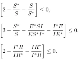
(24)
IAENG International Journal of Applied Mathematics, 46:2, IJAM_46_2_06
Since the arithmetic mean is greater or equal to the geometric mean (AM-GM inequality), one sees that
2−S ∗
S − S S∗
≤0,
3−S ∗
S − E∗SI ES∗I∗ −
I∗E IE∗
≤0,
2−I ∗R
IR∗ −
IR∗ I∗R
≤0.
It follows from (24) that L˙ ≤ 0 with L˙ = 0 if and only if S = S∗, E = E∗, I = I∗, R = R∗. Thus, by Lyapunov-LaSalle’s invariance principle [24], the largest compact invariant subset of the set where L˙ = 0 is the singleton{Ee= (S∗, E∗, I∗, R∗)}and we conclude that the
endemic equilibrium, Ee, is globally asymptotically stable.
This completes the proof.
The epidemiological implication of the above result is that the disease will establish itself in the community whenever
R0 > 1 irrespective of the initial sizes of the infectious
individuals in the population (see Figure 3 for a graphical illustration).
V. SENSITIVITY ANALYSIS AND SIMULATIONS
This section examines the changing effects of the model parameters with respect to the basic reproduction number,
R0, of the model (3). Numerical simulations are also carried
out to complement the theoretical results obtained.
A. Sensitivity Analysis
To determine how changes in parameters affect the trans-mission and spread of the disease with pseudo-recovery, a sensitivity analysis of the model (3) is carried out in the sense of [22], [27].
Definition 1. The normalized forward-sensitivity index of a variable, v, that depends differentiably on a parameter, p, is defined as:
Υvp =∂v
∂p × p
v. (25)
In particular, sensitivity indices of the basic reproduction number, R0, with respect to the model parameters are
examined. For examples, using (25), we obtain:
ΥR0
θ =
∂R0
∂θ × θ
R0
= θγ
(θ+µ)(θ+γ+µ),
ΥR0
γ =
∂R0
∂γ × γ
R0
=−
γ
γ+θ+µ
,
ΥR0
α =
∂R0
∂α × α
R0
= µ
α+µ.
(26)
The sensitivity index (S.I.) of R0 to µ can be obtained in
a similar manner and the signs of S.I. are summarized in the Table I. The positive sign of S.I. of R0 to the model
parameters shows that an increase (or decrease) in the value of each of the parameter in this case will lead to an increase (or decrease) in R0 of the model (3) and asymptotically
[image:6.595.101.239.81.183.2]results into persistence (or elimination) of the disease in the community (see, Theorem 4 and Theorem 5). For instance,
TABLE I SIGNS OFS.I.OFR0
Parameter S.I. β positive µ negative
α positive θ positive γ negative
TABLE II
THEVALUES OF MODEL PARAMETERS
Parameter Value Source β 0.1 [15] µ 0.01 [15] α varied Assumed θ varied Assumed γ 0.6 [11]
ΥR0
β = 1 means that increasing (or decreasing) β by 10%
increases (or decreases) R0 by 10%. On the contrary, the
negative sign of S.I. ofR0to the model parameters indicates
that an increase (or decrease) in the value of each of the parameter in this case leads to a corresponding decrease (or increase) in R0 of the model (3). Hence, with sensitivity
analysis, one can get insight on the appropriate intervention strategies to prevent and control the spread of the disease described by model (3).
B. Simulations
We illustrate the results of the sensitivity analysis by numerically simulating the behaviour of the model (3) using the parameter values given in Table II. In particular, we illustrate the changing effects of the pseudo-recovery rate, θ, and that of α on the size of infectious individuals. This is done because an increase or decrease in the basic reproduction number,R0, is determined by the influx of the
infectious individuals in the community.
Considering the initial conditions S0 = 0.99, E0 =
0.01, I0 = 0, R0 = 0, the results of the simulations are
provided in the Figures 1-3.
VI. CONCLUSION
This study presented both theoretical and quantitative analyses of a deterministic epidemiological model that is characterized by pseudo-recovery phenomenon. The results obtained are highlighted as follows:
(i) The disease-free equilibrium is locally asymptotically stable when the threshold quantity,R0, is less than unity.
(ii) The transcritical bifurcation at the threshold,R0= 1, is
forward and a locally asymptotically stable endemic equilib-rium exists whenR0>1as the threshold,R0, crosses unity.
(iii) The model has a globally asymptotically stable disease-free equilibrium when the threshold parameterR0<1.
(iv) The endemic equilibrium of the formulated model is globally asymptotically stable whenever the threshold quan-tity,R0, is greater than unity.
(v) Increasing the value of any of the parameters, β, α, or θ, increases the basic reproduction number, R0, and the
magnitude of the infectious individuals in the community
IAENG International Journal of Applied Mathematics, 46:2, IJAM_46_2_06
Fig. 1. The changing effects of the pseudo-recovery rateθon the number of infectious individuals. For a fixed valueα= 0.02withθ= 0.01(R0=
0.2151): (solid curve) andθ= 0.05(R0 = 0.6061): (dotted curve), the
[image:7.595.85.266.54.235.2]solutions approach the disease-free equilibrium asymptotically (in line with Theorem 4)
Fig. 2. The changing effects of the progression rateαon the number of infectious individuals. For a fixed valueθ= 0.05withα= 0.02(R0 =
0.6061) : (solid curve) and α = 0.04(R0 = 0.7272): (dotted curve)
which are in line with the sensitivity analysis results, increasing value ofαincreases the magnitude of the infectious individuals that eventually approach the disease-free equilibrium (in line with Theorem 4)
increases accordingly. Conversely, increasing the value of either µ or γ, decreases the basic reproduction number,
R0, and the magnitude of the infectious individuals in the
community decreases accordingly.
Therefore, it is pertinent to conclude that efforts at re-ducing the basic reproduction number of a disease should be encouraged in order to achieve a disease-free population. Above all, prevention, early detection and arresting any disease with or without pseudo-recovery at its onset is a panacea for the disease endemicity.
ACKNOWLEDGMENT
The improvement of the original manuscript is due to the constructive comments and valuable suggestions of the reviewers and handling editor.
Fig. 3. The changing effects of initial conditions as R0 > 1. For
fixed values of α = 0.02 with θ = 0.25; (R0 = 2.0155), and S0 = 0.99, E0 = 0.01, I0 = 0, R0 = 0: (solid curve), S0 = 0.97, E0 = 0.01, I0 = 0.02, R0 = 0: (dotted curve), S0 = 0.95, E0 = 0.01, I0 = 0.04, R0 = 0: (dashed curve). The
solutions asymptotically approach the endemic equilibrium (in line with Theorem 5)
REFERENCES
[1] W. O. Kermack and A. G. McKendrick, “Contributions to the mathe-matical theory of epidemics, part I,”Proceedings of the Royal Society of London Series A, vol. 115, 700–721, 1927.
[2] H. W. Hethcote, “The mathematics of infectious diseases,” SIAM Review, vol. 42, no. 4, pp. 599–653, 2000.
[3] M. Zhien, Z. Yicang and W. Jianhong,Modeling and Dynamics of Infectious Disease, World Scientific Publishing Co Pte Ltd., Singapore, 2009.
[4] S. M. Garba, A. B. Gumel and N. Hussaini, “Mathematical analysis of an age-structured vaccination model for measles,” Journal of the Nigerian Mathematical Society, vol. 33, pp. 41–76, 2014.
[5] C. P. Bhunu and S. Mushayabasa, “Modelling the transmission dynam-ics of pox-like infections,” IAENG International Journal of Applied Mathematics, vol. 41, no. 2, pp. 141–149, 2011.
[6] S. Olaniyi and O. S. Obabiyi, “Mathematical model for malaria trans-mission dynamics in human and mosquito populations with nonlinear forces of infection,”International Journal Pure and Applied Mathemat-ics, vol. 88, no. 1, pp. 125–156, 2013.
[7] C. Xu and M. Liao, “Stability and bifurcation analysis in a SEIR epidemic model with nonlinear incidence rates,”IAENG International Journal of Applied Mathematics, vol. 41, no. 3, pp. 191–198, 2011. [8] D. Tudor, “A deterministic model for herpes infections in human and
animal populations,”SIAM Review, vol. 32, no. 1, pp. 136–139, 1990. [9] H. F. Huo and G. M. Qiu, “Stability of a mathematical model of malaria transmission with relapse,”Abstract and Applied Analysis, vol. 2014, Article ID 289349, 9 pages, 2014.
[10] R. Xu, “Global dynamics of an SEIRI epidemiological model with time delay,”Applied Mathematics and Computation, vol. 232, pp. 436– 444, 2014.
[11] P. Georgescu and H. Zhang, “A Lyapunov functional for a SIRI model with nonlinear incidence of infection and relapse,”Applied Mathematics and Computation, vol. 219, pp. 8496–8507, 2013.
[12] H. Cox, Y. Kebeda, S. Allamuratova, G. Ismailov, Z. Davletmuratova, G. Byrnes, C. Stone, S. Niemann, S. Rsch-Gerdes, L. Blok and D. Doshetov, “Tuberculosis recurrence and mortality after successful treatment: impact of drug resistance,”PLoS Med., vol. 3, no. 10, pp. 1836–1843, 2006.
[13] C. Vargas-De-Le´on, “On the global stability of infectious diseases models with relapse”, Abstraction & Application, vol. 9, pp. 50-61, 2013.
[14] P. Guo, X. Yang and Z. Yang, “Dynamical behaviors of an SIRI epidemic model with nonlinear incidence and latent period,”Advances in Difference Equations, vol. 2014, pp. 164, 2014.
[15] A. Bernoussi, A. Kaddar and S. Asserda, “Global stability of a delayed SIRI epidemic model with nonlinear incidence,”International Journal of Engineering Mathematics, vol. 2014, Article ID 487589, 6 pages, 2014.
[16] P. van den Driessche and X. Zou, “Modeling relapse in infectious diseases,”Mathematical Biosciences, vol. 207, pp. 89–103, 2007.
IAENG International Journal of Applied Mathematics, 46:2, IJAM_46_2_06
[image:7.595.84.256.306.485.2][17] Z. Shuai and P. van den Driessche, “Global stability of infectious disease models using Lyapunov functions,”SIAM Journal on Applied Mathematics, vol. 73, no. 4, pp. 1513–1532, 2013.
[18] P. van den Driessche, L. Wang and X. Zou, “Modeling diseases with latency and relapse,”Mathematical Biosciences and Engineering, vol. 4, no. 2, pp. 205–219, 2007.
[19] P. van den Driessche and J. Watmough, “Reproduction numbers and sub-threshold endemic equilibria for compartmental models of disease transmission,”Mathematical Biosciences, vol. 180, no. 1-2, pp. 29–48, 2002.
[20] C. Castillo-Chavez and B. Song, “Dynamical models of tuberculosis and their applications,”Mathematical Biosciences and Engineering, vol. 1, no. 2, pp. 361–404, 2004.
[21] E. ´Avila-Vales, B. Buonomo and N. Chan-Chi, “Analysis of a mosquito-borne epidemic model with vector stages and saturating forces of infection,” arXiv:1402.1719v1, 2014.
[22] S. Olaniyi and O. S. Obabiyi, “Qualitative analysis of malaria dynam-ics with nonlinear incidence function,”Applied Mathematical Sciences, vol. 8, no. 78, pp. 3889–3904, 2014.
[23] A. Korobeinikov, “Global properties of infectious disease models with nonlinear incidence,” Bulletin of Mathematical Biology, vol. 69, pp. 1871–1886, 2007.
[24] J. P. LaSalle,The Stability of Dynamical Systems, Regional Conference Series in Applied Mathematics, SIAM, Philadelphia, Pa, USA, 1976. [25] C. Castillo-Chavez, S. Blower, P. van den Driessche, D. Kirschner and
A. Yakubu,Mathematical Approaches for Emerging and Reemerging Infectious Diseases: Models, Methods and Theory, Springer, New York, 2002.
[26] M. A. Safi and S. M. Garba, “Global stability analysis of SEIR model with holling type II incidence function,” Computational and Mathematical Methods in Medicine, vol. 2012, Article ID 826052, 8 pages, 2012.
[27] S. Mushayabasa and C. P. Bhunu, “Modeling HIV transmission dynamics among male prisoners in sub-saharan africa,”IAENG Inter-national Journal of Applied Mathematics, vol. 41, no. 1, pp. 62–67, 2011.