82
Increased interest in commodities, known as ‘com-modity financialization’, has generated a gradual integra-tion of agricultural commodity markets over the last decades, also influencing a rapid and steady growth of financial investments in these markets. Hamadi et al. (2017) contended that the so-called financialization of agricultural commodities took effect between 2004 and 2005. Numerous authors, such as Matošková (2011), Irwin and Sanders (2012) and Hernandez et al. (2014) claimed that agricultural commodity financialization had risen levels of correlation and volatility spillover among these assets. Hernandez et al. (2014) asserted that agricultural markets are highly interrelated and there are both own- and cross-volatility spillovers and dependence among most of the agricultural markets. Baldi et al. (2016) analysed agricultural commodities from the investors´ point of view. They asserted that investing in agricultural commodities is generally at-tributed to low correlation and interdependence with
traditional asset classes, such as stocks and bonds, which allows for portfolio diversification benefits. This happens due to the fact that agricultural commodities are driven by some particular fundamentals, e.g. weather condi-tions, supply constraints in the physical production, various geopolitical events, higher oil prices, increasing demand for biofuels, and speculation, which impose different price patterns and dynamics to agricultural commodities in respect to traditional assets.
In the process of the dynamic correlation investigation between various assets, most researchers observed this interconnection only via time dimension (Ceylan and Gozde 2012), neglecting the frequency domain features, which is an important aspect for investors who act at different time horizons. Conlon and Cotter (2012) ex-plained that the sample reduction problem arises when researchers try to match the frequency of data with the different time horizons, thus the multiscale analysis in the economy has been little studied in general.
Multiscale interdependence between the major
agricultural commodities
Dejan Živkov
1*, Jovan Njegić
1, Marko Pećanac
21Novi Sad Business School, Novi Sad, Serbia
2Office of the President of Republic of Serbia, Belgrade, Serbia *Corresponding author: [email protected]
Citation: Živkov D., Njegić J., PećanacM. (2019): Multiscale interdependence between the major agricultural commodities. Agricultural Economics – Czech, 65: 82–92.
Abstract: This paper investigates multiscale dynamic interconnection between the five agricultural commodities – corn, wheat, soybean, rice and oats, covering more than 18 years period. For research purposes, two complementary methodologies were used – wavelet coherence and phase difference. Low coherence is present at shorter time-horizons, while at longer time-horizons high coherence areas are found, but they are not widespread in all wavelet coherence plots. These results speak in favour of diversification opportunities. Strong coherence in longer time-horizons indicates that common factors are likely to be the main determinants of the agricultural prices in the long-run. On the other hand, rare high coherence areas at lower scales suggest that monetary and financial activities are most likely the causes that have affected the comovements of the grain prices in the short-term horizons. Phase difference discloses a relatively stable pattern between corn-soybean, corn-wheat, rice-oats and oats-soybean in the longer time-horizons. Taking into account investors’ diversification benefits and the leading (lagging) connections in long-run, corn and oats are the most appropriate cereals to be combined in an n-asset portfolio, since these two cereals constantly and very steadily lag soy-bean, whereas strong coherence between corn and oats does not frequently occur in all wavelet scales.
In addition, very little is known about the mutual interdependence across agricultural commodities, according to Trujillo-Barrera et al. (2012), and there is even less knowledge about their dynamic nexus at higher scales. In that regard, this study endeavours to contribute to the literature by investigating thor-oughly the nature of the dynamic interconnectedness between each pair of the five selected cereal spot commodities – wheat, corn, soybean, rice and oats, emphasising both time and frequency characteristics of their mutual nexus. Being sufficiently aware of the nature of the interlink between the selected agricultural commodities could serve well for various investors who combine agricultural commodities in their n-asset portfolio and act at different time-horizons. In order to provide such results, a wavelet coherence (WTC) method was used, which addresses both time and fre-quency domains, circumventing at the same time the problem of sample size reduction. The idea to utilise this method was borrowed from recent studies such as Barunik and Vacha (2013), Živkov et al. (2018) and Živkov et al. (2019). Dewandaru et al. (2014) claimed that the WTC methodology is particularly useful when researchers work with non-stationary signals that contain numerous outliers. In addition, the phase dif-ference method of Aguiar-Conraria and Soares (2011) was applied to furtheranalyse the lead/lag relation-ship between each examined pair of selected cereals in order to capture their spillover interconnections at particular time scale. To the best of our knowledge, very few papers scrutinised the interdependence among agricultural commodities, and none of the existing papers did an in-depth analysis of correlation and spillover effects via different frequency scales that exist between major cereal markets.
LITERATURE REVIEW
Since agricultural commodity prices began to exhibit considerably erratic behaviour between 2007–2008, the evolution of these movements has attracted attention in the media and academia alike. These markets are becoming more integrated because of globalisation, according to Sanjuan-Lopez and Dawson (2017), and thus the information about prices in one market is im-mediately transmitted electronically to others. Gilbert (2010a) contended that the demand for grains and oilseeds as biofuel feedstocks had been cited frequently as the main cause of the price rise. However, he found that the index based investment in agricultural futures markets is seen as the major channel through which
the macroeconomic and monetary factors generated the 2007–2008 food price rises. Gilbert (2010b) ar-gued that the observed change in food prices might be explained by financial activity in futures markets and various proxies for speculation. Adammer et al. (2017) analysed the long and short-run connection between North American and European agricultural futures markets. They found that the US markets lead in terms of price transmissions and volatility spillovers, but US markets, also, predominantly react to devia-tions from the long-run equilibrium which indicates a rising impact of the European agricultural markets.
The manuscript of Grieb (2015) investigated volatility spillover effects between nine physical commodity fu-tures contracts (corn, rough rice, soybeans, wheat, feeder cattle, lean hogs, live cattle, West Texas Intermediate (WTI) oil and Henry Hub natural gas). He revealed a strong pattern of price spillovers, while corn demon-strated to be the commodity that most broadly received and transmitted both price and volatility spillovers, fol-lowed by crude oil. The results of Lahiani et al. (2014) concur in a great extent with the findings of Grieb (2015). They examined the return and volatility spillovers among the four major agricultural commodities (wheat, sugar, cotton and corn). Results indicated that there is evi-dence of significant return and volatility transmission across considered commodities and that the conditional volatility of corn has an important explanatory power on the volatility of the other commodities. The paper of Musunuru (2014) analysed price volatility linkages between two important agricultural commodities: corn and wheat. He found evidence of bidirectional linkages between corn and wheat in terms of returns and volatility, while multivariate conditional Student’s
t-distribution results show a unidirectional volatility transmission from corn to wheat.
WAVELET COHERENCE AND PHASE DIFFERENCE
The wavelet technique estimates the spectral char-acteristics of a time-series as a function of time, re-vealing how the different periodic components of a specific time-series evolve. According to Dajčman (2012), the continuous wavelet transform Wx(u, s) is obtained by projectinga specific wavelet ψ(.) onto the examined time series x(t) which belongs to the Hilbert space L2 (R) by the following expression:
,
1 ψx t u
W u s x t dt
s s
where u represents the position of the wavelet in the time domain while s portrays the position in the frequency domain for a discrete time series x(t), t = 1, 2, …, N. From Equation 1, information on time and frequency can be simultaneously obtained by mapping the original time series into a function of u and s in the wavelet transform.
According to Vacha and Barunik (2012), squared wavelet coherence measures the local linear correlation between two stationary time series at each scale, and it is equivalent to the squared correlation coefficient in linear regression. Torrence and Webster (1999) explained that WTC can be presented as a squared absolutevalue of the smoothed cross wavelet spectra normalised by the product of the smoothed individual wavelet power spectra of each selected time series. The cross wavelet transform of two time-series, x(t) and y(t), is defined as W u sxy
, W u s W u sx
, y , , wherein Wx and Wy are the wavelet transforms of x and y, re-spectively. The squared wavelet coherence coefficient is given as follows:
2 1 2 2 2 1 1 , , , , xy x yS s W u s R u s
S s W u s S s W u s
(2)
where S(.)stands for a smoothing operator and s is a wavelet scale.The squared wavelet coherence coeffi-cient ranges at 0 ≤ R2(u, s) ≤ 1, whereby the values near zero point to weak correlation, while the values near one indicate a strong correlation. WTC is estimated by applying the Monte Carlo simulation methods.
One well-known lack of the WTC methodology is that it is unable to determine whether the dependence be-tween two time-series is positive or negative because the wavelet coherence is squared. Therefore, wavelet coherence phase differences that enable to see details on the delays in the oscillation (cycles) between two agricultural time-series under study were additionally considered. Following Torrence and Webster (1999) the wavelet coherence phase difference is defined as follows:
1 1 1 , , tan , xy xy xyS s W u s u s
S s W u s
I
R (3)
whereI and R are the imaginary and real parts,
re-spectively, of the smooth power spectrum. The phase difference between the two series (x, y) is indicated by vector arrows on the wavelet coherence plots. Vacha and Barunik (2012) contended that right (left) point-ing arrows indicate that the time series are in-phase (anti-phase) or are positively (negatively) correlated.
If arrows point to the right and up, the second vari-able is lagging and if they point to the right and down, the second variable is leading. Reversely, if arrows point to the left and up, the second variable is leading and if arrows point to the left and down, the second variable is lagging.
In addition, according to the explanation of Aguiar-Conraria and Soares (2011), if φxy∈ (0, π/2) then the series move in phase,with the time-series y leading x. On the contrary, if φxy∈ (−π/2, 0) then it is x thatis leading. An anti-phase situation (analogous to negative covariance) happens if there is aphase differ-ence of π (or −π), meaning φxy∈ (−π/2, π]
∪
(−π, π/2]. If φxy∈ (π/2, π) then xis leading, and the time series y is leading if φxy∈ (−π, −π/2). The phase difference of zero indicates that the time series move together (analogous topositive covariance) at the specified frequency.DATASET AND PRELIMINARY FINDINGS For the research purposes, the spot closing pric-es of the five major agricultural commoditipric-es were considered – corn, wheat, soybeans, rice and oats. All daily agricultural prices are transformed into ln-returns according to ri,t = 100 × ln(Pi,t/Pi,t–1), where ri,t is the agricultural return and Pi,t is the closing price of a particular agricultural commodity at time t. The sample covers the period from January 1, 2000 to February 28, 2018, and all data were obtained from the Datastream (2018). Utilizing the wavelet coher-ence methodology, dynamic nexus in seven frequency levels was investigated, allowing us to observe dynamic interconnection in seven different time horizons, which corresponds to: scale 1 (2–4 days), scale 2 (4–8 days), scale 3 (8–16 days), scale 4 (16–32 days), scale 5 (32–64 days), scale 6 (64–128 days) and scale 7 (128–256 days). First two scales observe the short-term dynamics, midshort-term is represented by the third, fourth and fifth scales, while the sixth and seventh scales correspond to the long-term dynamics.
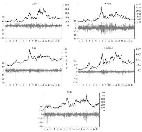
Table 1. Summary statistics of selected agricultural commodities
Mean Standard deviation Skewness Kurtosis JB
Corn 0.013 1.844 –0.620 15.691 29 234
Wheat 0.010 2.034 0.133 4.950 695
Soybean 0.016 1.713 –1.019 20.465 55 576
Rice 0.021 1.699 –0.551 17.278 36 823
Oats 0.016 2.458 –1.126 14.791 25 906
JB – value of Jarque-Bera coefficients of normality Source: authors’ calculation
Figure 1. Empirical dynamics of selected agricultural commodities
X-axis stands for years, left Y-axis denotes percentage, while right Y-axis indicates the price of the agricultural commodities; grey line denotes log returns of the agricultural commodities, while black line explains the empirical dynamics of the agricul-tural prices
Source: authors’ calculation
20 10 0 –10 –20 –30
20 10 0 –10 –20 –30
20 10 0 –10 –20 –30
20 10 0 –10 –20 –30 1 000
800 600 400 200 0
1 400 1 200 1 000 800 600 400 200
1 2 3 4 5 6 7 8 9 10 11 12 13 14 15 16 17 1 2 3 4 5 6 7 8 9 10 11 12 13 14 15 16 17
1 2 3 4 5 6 7 8 9 10 11 12 13 14 15 16 17 1 2 3 4 5 6 7 8 9 10 11 12 13 14 15 16 17
1 2 3 4 5 6 7 8 9 10 11 12 13 14 15 16 17 10
5 0 –5 –10 –15
10 5 0 25 20 15
30
2 000 1 600
1 200 800
400
600 500 400 300 200 100 0
Corn Wheat
Rice
Oats
[image:4.595.64.531.240.675.2]high, which mitigates diversification possibilities in the agricultural markets. Table 1 reveals that the highest average returns are obtained in rice, while standard deviation values indicate that oats are the riskiest agricultural commodity. Left skewness and high kurtosis are dominant among selected assets, which justifies the usage of wavelets, since this methodology can tackle outliers, but also can remove noises in the original data (Dewandaru et al. 2014). The JB test confirms the non-normality characteristics of agri-cultural commodities.
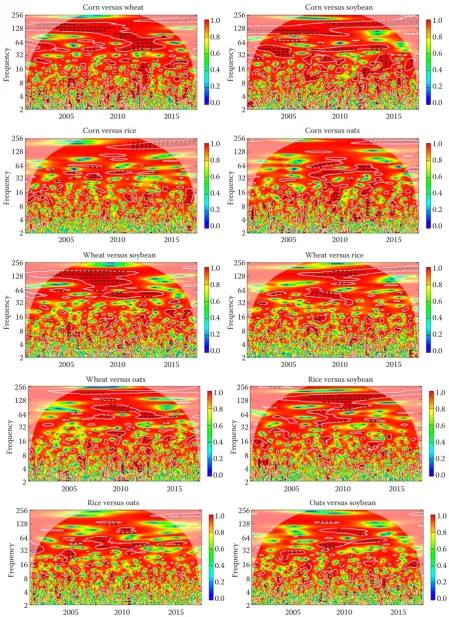
WAVELET COHERENCE RESULTS This section presents the results of the pairwise wavelet coherence1 plots between the five selected agricultural commodities. The wavelet technique can assess the strength of the interdependence both in time and frequency domains. The horizontal axis denotes time component in our WTC plots, while the left vertical axis represents the frequency component, which goes up to the seventh scale (256 days). The strength of the co-movement between each of the selected agricultural commodities is gauged via col-our surfaces, whereby blue and green colcol-ours signify low coherence, while warmer colours point to higher coherence. The colour pallet is presented at right Y-axis, and it ranges from 0 to 1. The cone of influ-ence marks the area of statistical significance at the 5% level obtained from the Monte Carlo simulations. Figure 2 reveals that cooler, that is, low correla-tion colours are dominant at high-frequency scales in all WTC plots. It implies that market-specific or idiosyncratic characteristics prevail in short-term. Although relatively unison movements of daily agri-cultural prices are found in Figure 1, the WTC plots do not show that a strong correlation exists between agricultural commodities at higher frequency scales, that is, shorter time-horizons. These results are in line with the findings of Sanjuan-Lopez and Dawson (2017), who contended that market microstructure models and the efficient markets hypothesis tend to have a major role in agricultural markets, whereby both private and public information becomes immediately compounded in prices because of electronic trading. Our results indicate that strong coherence islands are present between some agricultural commodities, but it appears evident only at higher wavelet scales, i.e. from 32 days onwards. For example, it is particularly
apparent for the corn-wheat, corn-soybean, wheat-soybean, wheat-rice and rice-soybean cases. High coherence at lower frequency scales suggests that fundamentals rather than idiosyncratic factors most likely mould the dynamics and the interrelationship between the selected cereals. This stance is in line with the findings of Gilbert (2010a), who contended that common factors, relating to demand growth, monetary and financial developments, are likely to be the main determinants of changes at the overall level of agricultural prices. In addition, he claimed that oil price and the dollar exchange rate movements had been important causal factors as well, but the impact of the former has varied over time, whereas exchange rate effects are relatively small.
High coherence areas are visible at higher scales, but it should be said that, in some instances, high correla-tions are visible even at the low scales, up to 32 days. Most striking cases in which higher coherence is visible at higher frequencies are corn-wheat, corn-soybean, corn-oats and wheat-oats. These findings could lead to the assumption that monetary and financial activi-ties could have some influence occasionally on grain prices over recent years. According to Figure 1, the boom in agricultural prices occurred in the 2006–2008 period, which took place in the context of enormous world liquidity, resulting from large US trade deficits and loose monetary policies. In the ‘post-Lehman’ months, the majority of the agricultural commodities prices saw sharp falls over the second half of 2008, which instigated high coherence as well. However, these results most likely do not reflect a direct causal link between agricultural assets, but rather common causation is a probable culprit. The increased interest in commodities, as a favourable asset class, before the world financial crisis was mostly stimulated by the general rise of energy, metal and agricultural prices. Agricultural investments are the activities that are sufficiently large to move prices and to induce nega-tive shocks to the limited agricultural inventories, galvanizing the inflation of food commodity prices. By all odds, the strong agricultural comovement does not happen immediately, but it comes at some delayed period, that is, at higher wavelet scales. However, in some cases, high coherence areas can be found even at the higher frequencies, but these are isolated phenomena. High coherence at lower wavelet scales might be the aftermath of the financial activity in fu-tures markets and various proxies for speculation
Figure 2. Pairwise wavelet coherence plots between five agricultural commodities
as explained by Cipra (2010) and Gilbert (2010b). Von Braun and Tadesse (2012) supported this stance, arguing that speculation effects could be stronger than demand- and supply-side shocks.
From the investors’ perspective, our WTC findings may indicate which agricultural commodities would serve well for diversification purposes in an n-asset portfolio. For investors who rebalance their portfolio in the short term (up to three weeks), all analysed cereals can be comprised in a portfolio, since all agri-cultural commodities have very low coherence between themselves at high frequencies. On the contrary, in-vestors who take their positions at somewhat longer time-period must contemplate more carefully which agricultural commodities are convenient to combine in a portfolio and which ones should be avoided, due to the presence of strong coherence that exists between some cereals at higher wavelet scales. For instance, our WTC results suggest that long term investors should not combine in one portfolio following pairs – corn and wheat, corn and soybean, wheat and soybean, and rice and soybean. One combination that particularly stand out among others and which would be suitable for all investors, regardless of which time-horizon they pursue, is a corn-rice pair. This pair has the lowest level of high coherence areas at all wavelet scales according to the WTC plots, whereas rice-oats, oats-soybean and corn-oats follow.
PHASE DIFFERENCE RESULTS
WTC plots provide good insight regarding the strength of coherence, which is an important in-put for the effective diversification realization. Also, WTC plots bear some information regarding the lead/lag relationship between the analysed series, and it is stored in phase-arrows of the WTC plots. One shortcoming with phase-arrows is that they can be seen only in strong coherence areas, while in other, lower coherence regions, phase arrows shift direction
constantly, without a common and stable behaviour.
In such circumstances, researchers cannot precisely make out which variable is lagging or leading the other one at higher frequency scales.In addition, it should be said that a strong minimal phase difference does
not exist under minimum dependency. So, in order
to avoid the phase difference biases,phase difference2 was calculated only at longer terms, because WTC plots suggest a stronger presence of high coherence
at longer time-horizons. This particular method car-ries the information regarding the direction of the
coherence, discloses the average lead/lag
relation-ship dynamics through the entire sample-period, and
ultimately indicates from which agricultural market
spillover shocks originate. Dajčman (2013) addressed
this issue, explaining that this information is useful
for international investors since if they know
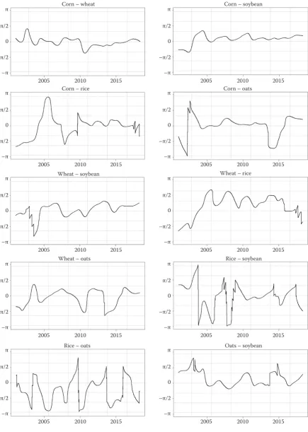
empiri-cally that one time-series leads the other one, then its realisations may be used to forecast the realisations of the lagging time series.Figures 3–4 present phase difference plots between the selected agricultural commodities at the 64–128 and 128–256 days fre-quency bands.
Figures 3–4 depict pairwise phase difference dynam-ics at the frequency range of 64–128 and 128–256 days, and it is obvious that shapes of phase differences in Figures 3–4 are relatively stable and long-lasting. All these characteristics create a good foundation for the appraisal of the lead/lag relationship between selected cereals since this information could be of a paramount significance for investors in terms of invest-ments in agricultural markets and portfolio selection. When it is clear which variable empirically leads the other one, then this information may be used to take an investment position in the lagging time series. With this type of knowledge, global investors can achieve higher returns in an n-asset portfolio.
Figure 3 describes the lead/lag nexus at the 64–128 days frequency band, and it can be seen that in some instances a stable and prolonged lead/lag patterns exist between some agricultural commodi-ties. For example, the most unambiguous relation has corn and soybean. Phase differences of these cereals are continuously above zero since 2002, which un-doubtedly suggests that developments in the soybean market precede the corn dynamics. Corn and wheat also have a relatively stable relationship since 2010, whereby corn is a commodity that has a leading role. In the case of corn and rice, rice leads corn since 2010. Striking dynamics can also be seen in the case of wheat and rice since 2003. In this case, phase difference has a very stable positive values from that year, which is clear indication that wheat is a lagging cereal. An interesting relationship have rice and oats, whereby it can be seen that phase difference frequently breaches –π/2 boundary, which is a sign that these two cereals found themselves quite often in an antiphase situation, and that is good for hedging purposes. In the cases of
Figure 3. Phase difference plots of agricultural commodities at 64–128 days frequency band
left Y-axis denotes phase difference domain, which spreads from π to –π Source: authors’ calculation
π
π/2
0
–π/2
–π
2005 2010 2015
Corn – wheat
π
π/2
0
–π/2
–π
2005 2010 2015
Corn – rice
π
π/2
0
–π/2
–π
2005 2010 2015
Wheat – soybean
π
π/2
0
–π/2
–π
2005 2010 2015
Wheat – oats
π
π/2
0
–π/2
–π
2005 2010 2015
Rice – oats
π
π/2
0
–π/2
–π
2005 2010 2015
Corn – soybean
π
π/2
0
–π/2
–π
2005 2010 2015
Corn – oats
π
π/2
0
–π/2
–π
2005 2010 2015
Wheat – rice
π
π/2
0
–π/2
–π
2005 2010 2015
Rice – soybean
π
π/2
0
–π/2
–π
2005 2010 2015
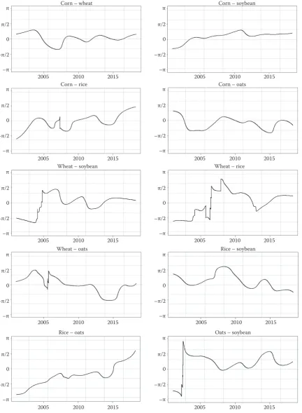
Figure 4. Phase difference plots of agricultural commodities at 128–256 days frequency band
left Y-axis denotes phase difference domain, which spreads from π to –π Source: authors’ calculation
π
π/2
0
–π/2
–π
2005 2010 2015
Corn – wheat
π
π/2
0
–π/2
–π
2005 2010 2015
Corn – rice
π
π/2
0
–π/2
–π
2005 2010 2015
Wheat – soybean
π
π/2
0
–π/2
–π
2005 2010 2015
Wheat – oats
π
π/2
0
–π/2
–π
2005 2010 2015
Rice – oats
π
π/2
0
–π/2
–π
2005 2010 2015
Corn – soybean
π
π/2
0
–π/2
–π
2005 2010 2015
Corn – oats
π
π/2
0
–π/2
–π
2005 2010 2015
Wheat – rice
π
π/2
0
–π/2
–π
2005 2010 2015
Rice – soybean
π
π/2
0
–π/2
–π
2005 2010 2015
other agricultural pairs, no steady lead/lag relation-ships were found at the sixth wavelet scale (64–128 days frequency band).
Figure 4 presents the phase difference results at the longest time-horizon. These findings seem very similar to the results found in Figure 3, but some discrepan-cies have also been reported. For instance, soybean constantly leads corn dynamics in the longest time-horizon, which is consistent with the findings pre-sented in Figure 3. On the other hand, in corn versus wheat plot, it is no longer so obvious which cereal has a dominant leading/lagging role, but it is more likely that both cereals follow the same homogeneous path, since the phase difference oscillates around zero from 2008. In the corn-rice and corn-oats plots, the results are pretty inconclusive, because lead/lag positions shift throughout the full-sample. It also applies for the wheat-soybean, wheat-rice, wheat-oats and rice-soybean pairs. At the 128–256 frequency band, rice and oats no longer report antiphase relations, which is different comparing to the findings in Figure 3. However, it is clear that rice has a dominant role till 2015, while from 2015 oats gains the upper hand. In the case of oats-soybean, it is apparent that phase difference is above zero since 2002, which suggests that soybean has a strong leading role from that year onwards.
CONCLUSION
This paper investigates the interdependence between the five spot agricultural commodities at different time-horizons. Two innovative and complementary methodologies were used – wavelet coherence and phase difference. The WTC results show the absence of strong coherence between agricultural commodities at higher frequency scales, but dark red islands were found between some agricultural commodities at longer time-horizons. High coherence at lower frequency scales suggests that common factors, that is, monetary and financial activities, are most likely the causes that have affected the comovements of the grain prices over the recent years. It is particularly apparent for the corn-wheat, corn-soybean, wheat-soybean, wheat-rice and rice-soybean cases.
The phase difference approach provides the in-formation regarding lead/lag relationship dynamics throughout the entire sample-period, and it shows from which agricultural market spillover shocks have
come from. This type of knowledge is particularly
useful for agricultural asset selection in terms of gain-ing profit, because the information about the leading
variable may be used to forecast the realisations of the lagging one. A stable pattern of the phase differ-ence can be seen at longer time-horizons, i.e. at the 64–128 and 128–256 frequency bands, whereby corn-soybean, corn-wheat, corn-rice and rice-oats are the pairs in which a clear and stable lead/lag relationship is present. More specifically, corn is the commodity that frequently lags most of all other listed cereals, while oats is a commodity that leads rice for most of the time.
Combining the findings from the wavelet coherence and phase difference methods, it can be suggested which cereals are the most appropriate to be found in an n-asset portfolio. According to evidence, at the 128–256 frequency band, corn and oats constantly and very steadily lag soybean. Therefore, observing the movements of soybean, future dynamics of corn and oats can be predicted, and thus these two cereals would be suitable elements in one portfolio. From the diversification point of view, corn and oats also have their advantages, since very low coherence is found between these two agricultural commodities in all the wavelet scales.
REFERENCES
Adammer P., Bohl M.T., von Ledebur E.O. (2017): Dynam-ics between North American and European agricultural futures prices during turmoil and financialization. Bulletin of Economic Research, 69: 57–76.
Aguiar-Conraria L., Soares M.J. (2011): Business cycle syn-chronization and the Euro: A wavelet analysis. Journal of Macroeconomics, 33: 477–489.
Baldi L., Peri M., Vandone D. (2016): Stock markets’ bubbles burst and volatility spillovers in agricultural commodity markets. Research in International Business and Finance, 38: 277–285.
Barunik J., Vacha L. (2013): Contagion among Central and Eastern European Stock Markets during the Financial Crisis. Finance a úvěr – Czech Journal of Economics and Finance, 63: 443–453.
Cipra T. (2010): Securitization of longevity and mortality risk. Finance a úvěr – Czech Journal of Economics and Finance, 60: 545–560.
Ceylan O., Gozde U. (2012): Cointegration and extreme value analyses of Bovespa and the Istanbul Stock Exchange. Fi-nance a úvěr – Czech Journal of Economics and FiFi-nance, 62: 66–90.
Dajčman S. (2012): The dynamics of return comovement and spillovers between the Czech and European stock markets in the period 1997–2010. Finance a úvěr – Czech Journal of Economics and Finance, 62, 368-390.
Dajčman S. (2013): Interdependence between some major European stock markets – A wavelet led/lag analysis. Prague economic papers, 22: 28–49.
Datastream (2018): Datastream. European University Insti-tute. Available at https://www.eui.eu/Research/Library/Re-searchGuides/Economics/Statistics/DataPortal/datastream Dewandaru G., Rizvi S.A.R., Masih R., Masih M., Alhabshi
S.O. (2014): Stock market co-movements: Islamic versus conventional equity indices with multi-timescales analysis. Economic Systems, 38: 553-571.
Gilbert C.L. (2010a): How to understand high food prices. Journal of Agricultural Economics, 61: 398–425.
Gilbert C.L. (2010b): Speculative Influences on Commodity Futures Prices 2006–2008. United Nations Conference on Trade and Development (UNCTAD). Discussion Pa-pers No. 197.
Grieb T. (2015): Mean and volatility transmission for commodity futures. Journal of economics and finance, 39: 100–118.
Hamadi H., Bassil C., Nehme T. (2017): News surprises and volatility spillover among agricultural commodities: The case of corn, wheat, soybean and soybean oil. Research in International Business and Finance, 41: 148–157. Hernandez M.A., Ibarra R., Trupki D.R. (2014): How far
do shocks move across borders examining volatility trans-mission in major agricultural futures markets. European Review of Agricultural Economics, 41: 301–325.
Irwin S.H., Sanders D.R. (2012): Financialization and struc-tural change in commodity futures markets. Journal of Ag-ricultural and Applied Economics, 44: 371–396.
Lahiani A., Nguyen D.K., Vo T. (2014): Understanding re-turn and volatility spillovers among major agricultural commodities. Journal of Applied Business Research, 29: 1781–1790.
Matošková D. (2011): Volatility of agrarian markets aimed at the price development. Agricultural Economics – Czech, 57: 34–40.
Musunuru N. (2014): Modeling price volatility linkages between corn and wheat: A multivariate GARCH esti-mation. International Advances in Economic Research, 20: 269–280.
Sanjuan-Lopez A.I., Dawson P.J. (2017): Volatility effects of index trading and spillovers on US agricultural futures markets: A multivariate GARCH approach. Journal of Ag-ricultural Economics, 68: 822–838.
Trujillo-Barrera A., Mallory M., Garcia P. (2012): Volatil-ity spillovers in U.S. crude oil, ethanol, and cornfutures markets. Journal of Agricultural and Resource Economics, 37: 247–262.
Torrence C., Webster P.J. (1999): Interdecadal changes in the ENSO-monsoon system. Journal of Climate, 12: 2679–2690. Vacha L., Barunik J. (2012): Co-movement of energy com-modities revisited: Evidence from wavelet coherence analy-sis. Energy Economics, 34: 241–247.
Von Braun J., Tadesse G. (2012): Global Food Price Volatility and Spikes: an Overview of Costs, Causes, and Solutions. ZEF-Discussion Papers on Development Policy No. 161. Živkov D., Balaban S., Đurašković J. (2018): What multiscale
approach can tell about the nexus between exchange rate and stocks in the major emerging markets? Finance a úvěr – Czech Journal of Economics and Finance, 68: 491–512. Živkov D., Đurašković J., Manić S. (2019): How do oil price
changes affect inflation in Central and Eastern European countries? A wavelet-based Markov switching approach. Baltic Journal of Economics, 19: 84–104.