A Spatial Sixth Order Finite Difference Scheme for Time Fractional Sub-diffusion Equation with Variable Coefﬁcient

(1)

A Spatial Sixth Order Finite Difference Scheme

for Time Fractional Sub-diffusion Equation with

Variable Coefficient

Shixiang Zhou, Fanwei Meng, Qinghua Feng

∗

, Li Dong

Abstract—In this paper, we present a finite difference scheme for a class of time fractional diffusion equation with variable coefficient, where the fractional derivative is defined by the Caputo derivative. The present algorithm is unconditionally stable, and possess spatial sixth order and temporal 2−α

order accuracy, which is an improvement of the spatial fourth order accuracy in the existing results. Theoretical analysis including local truncating error, unique solvability, stability and convergence for this algorithm is fulfilled. Then based on this finite difference scheme, we also investigate the construction of unconditionally stable finite difference scheme for a class of time fractional parabolic equation with spatial fourth derivative. In order to testify the efficiency of the algorithms as well as the convergence orders, some numerical examples are presented.

Index Terms—fractional sub-diffusion equation, difference scheme, variable coefficient, spatial sixth order accuracy, un-conditional stability.

I. INTRODUCTION

F

RACTIONAL differential equations containing the frac-tional derivative are widely used in various domains including physics, biology, engineering, signal processing, systems identification, control theory, finance, fractional dy-namics and so on (see [1,2] for example). In particular, the fractional derivative has proved to be very useful in describing the memory and hereditary properties of materials and processes. For the basic theory, readers can refer to the works [3,4]. One of its most important applications is to model the process of subdiffusion and superdiffusion of particles in physics, where the fractional diffusion equation is usually used for modeling this movement [5-7]. Recently, various aspects for fractional diffusion equations have been researched by many authors. In [8,9], the authors proposed certain methods for finding analytical solutions of fractional differential equations. In [10-12], qualitative and quantitative properties of solutions of fractional differential equations are investigated. In [13-15], the applications and physical mean-ing of fractional diffusion equations have been discussed, while numerical solutions for fractional diffusion equations are obtained by use of various methods including the finite element method [16,17], the meshless method [18,19], the finite difference method [20-30], the Bernstein polynomials

Manuscript received November 4, 2016; revised March 27, 2017. This work was partially supported by Natural Science Foundation of China (11671227), Natural Science Foundation of Shandong Province (China) (ZR2013AQ009) and the development supporting plan for young teacher in Shandong University of Technology.

S. Zhou, Q. Feng and L. Dong are with the School of Science, Shandong University of Technology, Zibo, Shandong, 255049 China; F. Meng is with the School of Mathematical Sciences, Qufu Normal University, Qufu, Shandong, 273165 China∗e-mail: [email protected]

method and so on [31]. Among the works for solving frac-tional diffusion equations, we notice that most of the current research for fractional diffusion equations is in constant coef-ficient case, and less attention has been paid to the research for fractional diffusion equations with variable coefficient. In [32], Chen et al. presented a fast semi-implicit difference method with convergence order O(τ+h) for a nonlinear two-sided space-fractional diffusion equation with variable diffusivity coefficients, and also developed a fast accurate iterative method by decomposing the dense coefficient matrix into a combination of Toeplitz-like matrices. In [33,34], the authors presented compact finite difference schemes with convergence order O(τ2−α ₊_h4₎ _(here ₀ _{< α <} ₁_{) for}

fractional sub-diffusion equation with the spatially variable coefficient subject to both Dirichlet boundary conditions and Neumann boundary conditions, and proved the stability and convergence order for the difference schemes. In [35], Wang established a compact finite difference method with convergence order O(τ3−α+τ2+h4) (here 1 < α < 2) for a class of time fractional convection-diffusion-wave e-quations with variable coefficients, while in [36], Wang et al. proposed a Petrov-Galerkin finite element method for variable-coefficient fractional diffusion equations, and proved the well-posedness and optimal-order convergence of this method. In [37], Anatoly et al. researched numerical methods for solving inverse problems for time fractional diffusion equation with variable coefficient.

In this paper, we consider the following time fractional sub-diffusion equation with variable coefficient and nonho-mogeneous source term

C

0D

α

tu(x, t) =

∂ ∂x(b(x)

∂u(x, t)

∂x ) +f(x, t), 0< α <1, (1)

which is subject to the following initial and periodic bound-ary value conditions

{

u(x,0) =φ(x), x∈R,

u(x, t) =u(x+L, t), x∈R, t∈[0, T], (2)

where the fractional derivative C

0Dαtu(x, t) =

1 Γ(1−α)

∫t

0

u′_t(x, s)

(t−s)αds is defined in the sense of Caputo

derivative, L is the period of u(x, t) with respect to the variable x, and b(x) is assumed to be smooth enough satisfyingb(x)≥L0>0.

The current work is devoted to deriving a finite difference scheme with spatial sixth order and temporal 2−α order accuracy for the above problems, and based on this finite

IAENG International Journal of Applied Mathematics, 47:2, IJAM_47_2_08

(2)

difference scheme we will also investigate the construction of unconditionally stable finite difference scheme for a class of time fractional parabolic equation with spatial fourth derivative as follows

C

0D

α

tu(x, t) +uxxxx=f(x, t), 0< α <1, (3)

which is subject to the following initial and periodic bound-ary value conditions (2).

We organize the rest of this paper as follows. In Section 2, we give the derivation of the finite difference scheme for solving fractional sub-diffusion equation (1) under the conditions (2). Then in Section 3, theoretical analysis of local truncating error, unique solvability, stability and convergence for the finite difference scheme are fulfilled. In Section 4, we apply the method in Section 2 to construct unconditionally stable finite difference scheme with spatial fourth order accuracy for Eq. (3). In Section 5, we give some numerical examples to verify the theoretically analytical results. In Section 6, some concluding statements are presented.

II. ESTABLISHMENT OF THE HIGH ORDER FINITE DIFFERENCE SCHEME FOREQ. (1)

Since the periodic boundary value condition is considered here, it is sufficient to assumex∈[0, L]. LetM, N be two positive integers, andh= _ML, τ= _NT denote the spatial and temporal step size respectively. Define xi =i∗h(0≤ i≤

M), tn=nτ(0≤n≤N), Ωh={xi|0≤i≤M}, Ωτ =

{tn|0 ≤ n ≤ N}, (i, n) = (xi, tn), and then the domain

[0, L]×[0, T] is covered by Ωh×Ωτ. Let Vh = {uni|0 ≤

i ≤ M, 0 ≤ n ≤ N} be the grid function on the mesh

Ωh×Ωτ.Uin=u(xi, tn) anduni denote the exact solution

and numerical solution at the point(i, n)respectively.Un₌

(U₁n, U₂n, ..., U_Mn)T, un= (un₁, un₂, ..., un_M)T.

In order to approximate the time derivative, the following lemmas are listed for further use.

Lemma 1 [33, Lem. 2.1](The L1 formula). Suppose

0< α <1, andu(t)∈C2[0, tn]. Then it holds that

| 1

Γ(1−α) ∫ tn

0

u′(s) (tn−s)α

ds− τ

−α

Γ(2−α)

[a(₀α)u(tn)− n−1 ∑

k=1

(a(_nα₋)_k₋₁−a_n(α₋)_k)u(tk)−a

(α)

n−1u(t0)]| ≤ 1

Γ(2−α)[ 1−α

12 + 22−α

2−α−(1+2

−α_{)] max} t0≤t≤tn

|u′′(t)|τ2−α,

(4)

wheret0= 0,a (α)

k = (k+ 1)

1−α₋_k1−α_{, k}_≥₀_.

Lemma 2. [38, Lem. 1.4.8] Suppose 0 < α < 1, anda(_kα), k≥0 are defined as in Lemma 2, then

{

1 =a(₀α)> a(₁α)> a₂(α)> ... > a(_kα)> ... >0,

lim

k→∞a

(α)

k = 0,

(5)

and

(1−α)k−α< a(_kα₋)₁<(1−α)(k−1)−α. (6)

Lemma 3. Supposeu(x, t)∈C(8,3)_([_x

i−3, xi+3]×[0, T]),

and define two operatorsH1, H2 such that

          

H1Uin= 1_h(−₆₀1 U n

i−3+ 3₂₀U

n

i−2−3₄U

n i−1 + 3₄U_in₊₁−₂₀3 U_in₊₂+ 1₆₀U_in₊₃),

H2Uin= 1_h2( 1₉₀Uin−3−₂₀3 Uin−2+ 3₂Uin−1−49₁₈Uin

+ 3₂U_in₊₁−₂₀3 U_in₊₂+ 1₉₀U_in₊₃),

(7)

where Un

i = u(xi, tn). Then ux and uxx can be

approx-imated by H1Uin and H2Uin respectively with sixth order

accuracy, that is,

  

|ux(xi, tn)−H1Uin| ≤ ₅84×_7! max xi−3≤x≤xi+3

|u(7)x (x, t)|h6,

|uxx(xi, tn)−H2Uin| ≤ 72_8! max x_i−3≤x≤xi+3

|u(8)x (x, t)|h6,

(8)

whereC1, C2 are two constants.

The proof of Lemma 3 can be completed by the expansion of the Taylor’s formula.

In order to establish the difference scheme, we rewrite Eq. (1) as

C

0D

α

tu(x, t) =b′(x)ux+b(x)uxx+f(x, t), 0< α <1, (9)

Denote ∆α

τUin = τ

−α

Γ(2−α)[a (α) 0 U

n i −

n∑₋1

k=1

(a(_nα₋)_k₋₁ − a(_nα₋)_k)Uk

i −a

(α)

n−1Ui0], where a

(α)

k , k = 0,1, ..., n−1 are

defined as in Lemma 1. Then it follows from Lemmas 1 and 3 that

∆α_τU_in=b′_iH1Uin+biH2Uin+f n i +R

n

i(τ, h), (10)

whereb′_i=b′(xi), bi=b(xi),fin=f(xi, tn), and

|Rn_i(τ, h)| ≤ 1

Γ(2−α)[ 1−

α

12 + 2 2−α

2−α −(1 + 2−α_{)] max}

t0≤t≤tn

|u′′_t(x, t)|τ2−α

+ 84

5×7!0max≤x≤L|u

(7)

x (x, t)|h6+ 72_8! max

0≤x≤L|u

(8)

x (x, t)|h6.

Then the difference scheme approximating Eq. (1) at the point (i, n) under the conditions (2) can be established as follows

  

∆α

τuni =b′iH1uni +biH2uni +fin, 1≤n≤N,

u0

i =φ(xi),

un

i =uni±M, 1≤i≤M, 1≤n≤N.

(11)

III. THEORETICAL ANALYSIS OF THE DIFFERENCE SCHEME

In this section, we fulfill analysis of local truncating error, unique solvability, stability and convergence for the finite difference scheme (11) by use of the Fourier analysis method.

IAENG International Journal of Applied Mathematics, 47:2, IJAM_47_2_08

(3)

A. Local truncating error and unique solvability

First the local truncating error for the difference scheme (11) can be directly obtained as O(τ2−α₊_h6₎_.

In order to facilitate fulfilling the analysis, we rewrite the first equation of the finite difference scheme (11) as the following form

[µ−180h2(b′iH1+biH2)]uni = n−1

∑

k=0 Bknu

k i+180h

2

fin,1≤i≤M,

(12)

where µ = 180h2τ−α Γ(2−α), B

n

0 = µa

(α)

n−1, Bkn =

µ(a(_nα₋)_k₋₁−a(_nα₋)_k), k= 1,2, ..., n−1,(b′_iH1+biH2)uni =

− 1

180h2[gi,i−3u

n

i−3+gi,i₋2uni−2 +gi,i₋1uni−1 +gi,iuni +

gi,i+1uni+1+gi,i+2uni+2+gi,i+3uni+3], 1 ≤ i ≤M, uni =

un

i_±M, and

                  

gi,i= 490bi,

gi,i+1=−135hb′i−270bi,

gi,i+2= 27hb′i+ 27bi,

gi,i+3=−3hb′i−2bi,

gi,i₋1= 135hb′i−270bi,

gi,i−2=−27hb′i+ 27bi,

gi,i−3= 3hb′i−2bi,

i= 1,2, ..., M. (13)

For the sake of using the Fourier analysis method, define

vn₍_x_{) =}

{

un

i, x∈[xi−1, xi+1

2), i= 1,2, ..., M−1,

un

M, x∈[xM−1, xM],

yn(x) = {

fn

i , x∈[xi−1, xi), i= 1,2, ..., M−1,

fn

M, x∈[xM−1, xM],

and a periodic extension is applied to vn₍_x₎_{, y}n₍_x₎_.

Then from Eq. (12) one can obtain that

[µ−180h2(b′iH1+biH2)]vn(x) =

n−1

∑

k=0 Bknv

k

(x) + 180h2yn(x).

(14)

where

(b′iH1+biH2)vn(x) =

b′i

h[−

1 60v

n₍_x₋₃_h_{) +} 3

20v

n₍_x₋₂_h₎

−3

4v

n₍_x₋_h₎₊3

4v

n₍_x₊_h₎₋ 3

20v

n₍_x₊₂_h₎₊ 1

60v

n₍_x₊₃_h_)]

+bi

h2[

1 90v

n₍_x₋₃_h₎₋ 3

20v

n₍_x₋₂_h_{) +}3

2v

n₍_x₋_h₎

−49

18v

n₍_x_{) +}3

2v

n₍_x₊_h₎₋ 3

20v

n₍_x_{+ 2}_h_{) +} 1

90v

n₍_x_{+ 3}_h_)]_.

The functionsvn₍_x₎_and_yn₍_x₎_{can be denoted by the Fourier}

series forms as follows

vn(x) = ∞ ∑

l=−∞ e

vnl exp( 2πlxj

L ), y

n (x) =

∞ ∑

l=−∞ e

ylnexp( 2πlxj

L ),

(15)

where

e

vn l = 1_L

∫L

0 v

n₍_x_{) exp(}₋2πlxj

L )dx,

e

y_ln= 1_L∫₀Lyn(x) exp(−2πlxj_L )dx, andj denotes the imaginary unit.

Define the discreteL2 norm by ∥un∥2 = (

M

∑

i=1

h|un i|2)

1 2.

Then by use of the Parseval’s equality one can obtain that

∥un_∥

2= ( ∫L

0 |v

n₍_x₎_|2_dx₎1 2 = (

∞ ∑

l=−∞

|ven l|2)

1 2,

∥fn_∥

2= ( ∫L

0 |y

n₍_x₎_|2_dx₎1 2 = (

∞ ∑

l=−∞

|yen l|

2₎1 2.

Substituting (15) into (14), and denoting p = 2_Lπl, we can get that

∞ ∑

l=−∞

{[µ−180h2(b′_iH1+biH2)] exp(pxj)}venl

= ∞ ∑

l=−∞ [

n₋1 ∑

k=0

B_knevk_l exp(pxj) + 180h2yen_l exp(pxj)]. (16)

Furthermore, after some basic computation, one can see that the following relations hold

−180h2₍_b′

iH1+biH2) exp(pxj) =

exp(pxj)[gi,i₋3exp(−3phj) +gi,i₋2exp(−2phj) +gi,i₋1exp(−phj) +gi,i+gi,i+1exp(phj) +gi,i+2exp(2phj) +gi,i+3exp(3phj)]

= exp(pxj)(q1+h2q2j), (17)

where

q1=−4[4 cos3(ph)−27 cos2(ph) + 132 cos(ph)−109]bi,

q2= [−270 sin(ph) + 54 sin(2ph)−6 sin(3ph)]b ′

i

h .

By a close observation onq1, q2one can deduce thatq1≥0,

q2 is continuous withouth= 0, and lim

h→0q2=−180pb ′

i.

So it follows from above that

∞ ∑

l=−∞

{[µ+ (q1+h2q2j)]evln}exp(pxj)

= ∞ ∑

l=−∞

{

n−1 ∑

k=0

B_knev_lk+ 180h2yen_l}exp(pxj). (18)

On the other hand, due to the orthogonality of

exp(2πlxj

L ), l = 0,±1,±2, ...,±∞, multiplying

exp(−pxj)on both sides of (18), and integrating from0 to Lwe get that

[µ+ (q1+h2q2j)]evln= n_∑−1

k=0

Bnkvekl + 180h2eynl,

l= 0,±1,±2, ...,±∞. (19)

Theorem 1. The finite difference scheme denoted by (11) is uniquely solvable.

Proof. In order to prove the unique solvability of (11), it is sufficient to prove that there is only zero solution for the corresponding homogeneous difference equation.

IAENG International Journal of Applied Mathematics, 47:2, IJAM_47_2_08

(4)

From the process above one can see that after fulfilling Fourier transformation, the following equation can be ob-tained due to the homogeneous difference equation

[µ+ (q1+h2q2j)]evnl = 0, (20)

which impliesev_ln= 0 due to|µ+ (q1+h2q2j)|>0.

So by (15) one hasvn₍_x_{) = 0}_{, and then}_∥_un_∥

2= 0, which

impliesun

i = 0, i= 1,2, ..., M. The proof is complete.

B. Stability

Theorem 2. For Eq. (19), it holds that

|evnl| ≤ |ev

0

l|+ (1 +τ) n

max

1≤s≤n|ye s l| ≤ |ev

0

l|+e T

max

1≤s≤n|ye s l|. (21)

Furthermore, the finite difference scheme denoted by (11) is unconditionally stable on the initial value and the right source termf(x, t).

Proof. We will use the mathematical induction method to prove (21).

Whenn= 1, from (19) it holds that

[µ+(q1+h2q2j)]ev1l =B

1

0evl0+180h

2_e_y1

l =µev

0

l+180h

2_y_e1

l,

which implies that

|ev1

l|=|

µev_l0+ 180h2ye1_l µ+ (q1+h2q2j)|

≤ √ µ

(µ+q1)2+h4q22

|ev0

l|+ 180h

2 √

(µ+q1)2+h4q22

|ye1

l|

≤ |ev0

l|+ Γ(2−α)τ α_|_y_e1

l| ≤ |ev

0

l|+τ α_|_e_y1

l|.

In the case τ≥1, one hasτα_≤_τ _≤_{1 +}_{τ, while in the}

case 0< τ <1, one has τα ≤1≤1 +τ. So τα≤1 +τ holds for∀τ >0. Then

|ve_l1| ≤ |ev_l0|+ (1 +τ)|ye1_l| ≤ |ev_l0|+eT|ey1_l|. So (21) holds for n= 1.

Suppose (21) holds for the time levels 1,2, ..., n− 1. Then for the time level n, from (19) one can deduce that

|evn_l|=|

n∑−1

k=0

Bnkev k

l + 180h

2_e

yln

µ+ (q1+h2q2j) |

≤ 1

|µ+ (q1+h2q2j)|

n∑−1

k=0

|B_kn||vek_l|+| 180h 2_e_yn

l

µ+ (q1+h2q2j)|

≤ 1

|µ+ (q1+h2q2j)|

n∑−1

k=0

|Bn

k||ve0l|+_|_µ_{+ (}_q 1

1+h2q2j)|

n∑−1

k=0 [|Bn

k|(1 +τ)k max

1≤s≤k|ye s l|] +|

180h2ye_ln µ+ (q1+h2q2j)|

=√ 1

(µ+q1)2+h4q22

n−1 ∑

k=0

|Bkn||ev0l|+

1 √

(µ+q1)2+h4q22

n∑−1

k=0

[|B_kn|(1 +τ)k max 1≤s≤k|ye

s l|] +|

180h2yen_l

√

(µ+q1)2+h4q22

|

≤_√ 1

(µ+q1)2+h4q22

n∑−1

k=0

|Bn k||evl0|

+

(1 +τ)n−1 max 1≤s≤n−1|ye

s l|

√

(µ+q1)2+h4q22

n_∑−1

k=0

|Bn_k|+| 180h 2_e_yn

l

√

(µ+q1)2+h4q22

|.

From Lemma 2 one can obtain

n∑−1

k=0

|Bn k|=µa

α

0 =µ. So

|evn l| ≤

µ

√

(µ+q1)2+h4q22

|ev0

l|+

µ

√

(µ+q1)2+h4q22

(1 +τ)n−1 _max 1≤s≤n−1|ey

s l|+|

180h2ye_ln

√

(µ+q1)2+h4q22

|

≤ |ev0

l|+ (1 +τ)n−1 max

1≤s≤n−1|ey

s l|+|

180h2ye_ln µ |

=|ev0

l|+ (1 +τ)n−1 max

1≤s≤n−1|ey

s

l|+ Γ(2−α)τα|eynl|

≤ |ev0

l|+ (1 +τ)n−1 max

1≤s≤n−1|ey

s

l|+ (1 +τ)|yeln|

≤ |ev0_l|+ (1 +τ)n max 1≤s≤n|ye

s l|

≤ |ev0_l|+enτ max 1_≤s_≤n|ye

s l|

≤ |ev0_l|+eT max 1_≤s_≤n|ey

s l|

So (21) holds according to the mathematical induction method.

By the Parseval’s equality, one can deduce that ∥un_∥

2 ≤

∥u0_∥

2 +eT max 1≤s≤n∥f

s_∥

2. So the finite difference scheme

denoted by (11) is unconditionally stable on the initial value and the right source termf(x, t). The proof is complete.

C. Convergence

Theorem 3. The finite difference scheme denoted by (11) is convergent.

Proof. Letηn

i =Uin−uni, i= 1,2, ..., M, n= 0,1, ..., N

denote the absolute error between the exact solutions and the numerical solutions, andηn= (η₁n, η₂n, ..., ηn_M)T. Then η_i0= 0, and from (10)-(12) one can deduce that

[µcn₀−180h2(b′_iH1+biH2)]ηni = n_∑₋1

k=0

B_knuk_i+180h2Rn_i(τ, h),

(22)

where|Rn

i(τ, h)|=O(τ2−α+h6).

Define

θn₍_x_{) =}

{

ηn

i, x∈[xi₋1, xi), i= 1,2, ..., M−1,

ηn

M, x∈[xM₋1, xM],

rn(x) = {

Rn_i(τ, h), x∈[xi−1, xi), i= 1,2, ..., M−1,

Rn_M(τ, h), x∈[xM−1, xM],

and a periodic extension is applied to θn(x), rn(x). The functions θn(x) and rn(x) can be denoted by the

IAENG International Journal of Applied Mathematics, 47:2, IJAM_47_2_08

(5)

Fourier series form as follows

θn₍_x_{) =} ∑∞ l=−∞

e

θn l exp(

2πlxj L ),

rn₍_x_{) =} ∑∞ l=−∞

e

rn l exp(

2πlxj L ),

where

e

θ_ln= 1_L∫₀Lθn(x) exp(−2πlxj_L )dx,

e

rn l = 1_L

∫L

0 r

n₍_x_{) exp(}₋2πlxj

L )dx.

Following in a similar manner as the proof of Theorem 2 one can get that

|θe_ln| ≤ |θe_l0|+eT max 1≤s≤n|er

s l|.

By η_i0= 0we have θe0_l = 0, and then |θe_ln| ≤eT max

1_≤s_≤n|er s l|.

Furthermore,

∥ηn∥2≤eT max 1≤s≤n∥R

s₍_{τ, h}₎_∥

2≤C(τ2−α+h6), (23)

whereC is a positive constant.

The convergence of the finite difference scheme (11) follows from (23), and the proof is complete.

IV. THE HIGH ORDER FINITE DIFFERENCE SCHEME FOR

EQ. (3)

In this section, we apply the concept of constructing high order finite difference scheme in Section 2 to a class of time fractional parabolic equation with spatial fourth derivative denoted by Eq. (3), and try to construct unconditionally stable finite difference scheme for it under the conditions (2).

In order to approximate the spatial derivative, the following lemma will be used.

Lemma 4. Supposeu(x, t)∈C(8,2)_([_x

i₋3, xi+3]×[0, T]),

and define one operator ϕsuch that

ϕU_in= 1

h4(−

1 6U

n i−3+ 2U

n i−2−

13 2 U

n i−1+

28 3 U

n i −

13 2 U

n i+1 +2U_in₊₂−1

6U

n

i+3), (24)

whereUn

i =u(xi, tn). Then it holds that

|uxxxx(xi, tn)−ϕUin| ≤

7

240x_i−3max≤x≤xi+3

|u(8)_x (x, t)|h4.

(25)

The proof of Lemma 4 can be completed by applying the expansion of the Taylor’s formula to the right term of Eq. (24).

By use of Lemmas 1 and 4, one has the following observation at the point(i, n)

τ−α

Γ(2−α)[a (α) 0 U

n i −

n∑−1

k=1

(a(_nα₋)_k₋₁−a(_nα₋)_k)U_ik−a(_nα₋)₁U_i0] +ϕUin=f

n i +R

n

i(τ, h), (26)

whereϕ is define as in Lemma 1,fn

i =f(xi, tn), and

|Rn_i(τ, h)| ≤ 1 Γ(2−α)[

1−α

12 + 22−α

2−α−(1 + 2

−α_)]

max

t0≤t≤tn

|u′′t(x, t)|τ2−α+

7

2400max_≤x_≤L|u

(8)

x (x, t)|h4.

So the finite difference scheme approximating Eq. (3) at the point (i, n) under the conditions (2) can be established as follows

          

τ−α

Γ(2−α)[a (α) 0 uni −

n∑−1

k=1

(a(_nα₋)_k₋₁−a(_nα₋)_k)uk i −a

(α)

n−1u0i]

+ϕun

i =fin, 1≤n≤N,

u0

i =φ(xi),

un

i =uni±M, 1≤i≤M, 1≤n≤N.

(27)

By use of the Fourier analysis method, similar to the process of Theorems 1-3, we have the following theorems.

Theorem 4. The finite difference scheme denoted by (27) is uniquely solvable.

Theorem 5. For the difference scheme (27), it holds that

∥un∥2≤ ∥u0∥2+eT max 1≤s≤n∥f

s_∥

2, n= 1,2, ..., N,

(28)

that is, the finite difference scheme denoted by (27) is unconditionally stable on the initial value and the right term f(x, t).

Theorem 6. The finite difference scheme denoted by (27) is convergent with spatial fourth order and temporal

2−αorder accuracy.

V. NUMERICAL EXPERIMENTS

In this section, we present some numerical examples for the present finite difference schemes. In the following, the maximum error at all grid points is denoted by

e(τ, h) = max 1≤n≤N|U

n₋_un_|_,

and the convergence orders in temporal direction and spatial direction are defined by

Rateτ =

ln(e(τ1, h)/e(τ2, h)) ln(τ1/τ2)

,

Rateh= ln(e(τ, h_ln(_h1)/e(τ, h2))

1/h2)

respectively.

Example 1. Consider the problems (1)-(2) with an exact analytical solutionu(x, t) = (t3+ 1) sin(2πx), where the period with respect to the variable x is L = 1, and satisfies

IAENG International Journal of Applied Mathematics, 47:2, IJAM_47_2_08

(6)

        

b(x) =x2+ 1,

u(x,0) =φ(x) = sin(2πx), f(x, t) = [ Γ(4)

Γ(4−α)t

3₋α_{+ 4}_π2₍_t3_{+ 1)(}_x2_{+ 1)]} sin(2πx)−4πx(t3_{+ 1) cos(2}_πx₎_.

In Fig. 1, the errors between the exact solutions and the nu-merical solutions under certain conditions are demonstrated, from which one can see that the errors between the numerical solutions and the exact solutions can be restricted to a low level. Even with the increasing of the time steps, the errors can also be maintained to an accepted level, which coincides with the stability analysis in Section 3.

[image:6.595.315.556.57.330.2]

The maximum errors and convergence orders in spatial direction after five time steps are listed in Tables 1-2.

Table 1: The maximum errors and convergence orders in spatial direction atτ= 0.01

α= 0.3 α= 0.5

h e(τ, h) Rateh e(τ, h) Rateh 1

10 1.245×10−

4

- 1.109×10−4

-1

12 4.040×10−

5

6.173 3.693×10−5 6.031

1

14 1.578×10−

5

6.097 1.460×10−5

6.018

1

16 7.022×10−

6

6.066 6.620×10−6 5.924

1

18 3.372×10−6 6.227 3.229×10−6 6.095 1

20 1.786×10−

6

[image:6.595.61.267.67.318.2]

6.033 1.754×10−6 5.795

Table 2: The maximum errors and convergence orders in spatial direction atτ= 0.001

α= 0.3 α= 0.5

h e(τ, h) Rateh e(τ, h) Rateh 1

10 1.153×10−

4

- 8.137×10−5

-1

12 3.820×10−5 6.062 2.764×10−5 5.922 1

14 1.506×10−

5

6.036 1.082×10−5 6.084

1

16 6.798×10−

6

5.958 4.964×10−6 5.836

1

18 3.289×10−

6

6.164 2.442×10−6

6.022

1

20 1.760×10−

6

5.935 1.296×10−6 6.011

The results in Tables 1-2 show that the convergence orders in spatial direction are about sixth order, which coincide with the theoretical analysis in Section 3.

Example 2. Consider the problems (2)-(3) with an exact analytical solutionu(x, t) = t1.7_cos(2_πx₎_{, where the}

periodL= 1 with respect to the variable x, and satisfies

{

u(x,0) = 0,

f(x, t) = [ 1.7Γ(1.7) Γ(2.7−α)t

β₋α₋₁₆_t1.7_π4_{] cos(2}_πx₎_.

The accuracy of the finite difference scheme is checked by comparing the exact solutions and the numerical solutions, which can be seen from the maximum error. Also the convergence orders in both spatial direction and temporal direction are obtained.

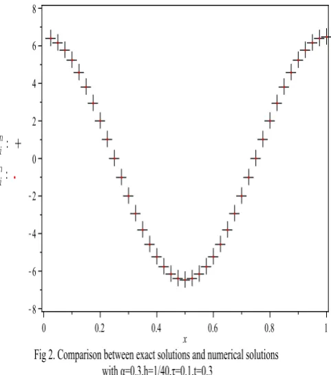
In Fig. 2, comparison between the exact solutions and the numerical solutions with different conditions is made, which shows that the numerical solutions can approximate the exact solutions satisfactorily.

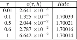
The maximum errors and convergence orders in spatial and temporal directions are listed in the following tables respectively, where t ∈ [0,1] in Table 3, while t ∈ [0,3]

in Table 4.

Table 3: The maximum errors and convergence orders in spatial direction atα= 0.3, τ = 0.1

h e(τ, h) Rateh 1

8 3.152×10−3 -1

10 1.325×10−

3

3.88523

1

15 2.673×10−

4

3.94707

1

20 8.385×10−

5 _4.03054

1

25 3.308×10−

5

4.16818

IAENG International Journal of Applied Mathematics, 47:2, IJAM_47_2_08

[image:6.595.57.283.542.785.2]

(7)

[image:7.595.105.235.85.153.2]

Table 4: The maximum errors and convergence orders in temporal direction atα= 0.3, h= 0.1

τ e(τ, h) Rateτ

0.01 2.641×10−5 -0.1 1.325×10−3 1.70039 0.5 2.044×10−2 1.70021 0.6 2.787×10−2 1.70016 1 6.642×10−2 1.70014

From the results in Tables 3-4 one can see that the convergence orders are fourth order and2−αorder roughly in spatial direction and temporal direction respectively, which coincide with the theoretical analysis in Section 4.

VI. CONCLUSIONS

In this paper, a new high order finite difference algorithm for solving a class of time fractional sub-diffusion equation with variable coefficient was developed. The present algorith-m is of spatial sixth order and tealgorith-mporal2−αorder accuracy. The unconditional stability and convergence for this algo-rithm were proved by use of the Fourier analysis method. This concept of constructing high order finite difference scheme was applied to a class of time fractional parabolic equation with spatial fourth derivative, and a high order unconditionally stable finite difference scheme for it was also proposed. In order to verify the validity of the present algorithms, numerical experiments were carried out, and the numerical results show their coincidence with the theoretical analysis. Finally, we note that this handling process can be applied to other fractional differential equations to develop corresponding finite difference algorithms with high order.

REFERENCES

[1] A. Bouhassoun, “ Multistage Telescoping Decomposition Method for Solving Fractional Differential Equations,”IAENG International Jour-nal of Applied Mathematics, vol. 43, no. 1, pp. 10-16, 2013. [2] A. M. Bijura, “ Systems of Singularly Perturbed Fractional Integral

Equations II,”IAENG International Journal of Applied Mathematics, vol. 42, no. 4, pp. 198-203, 2012.

[3] I. Podlubny, “Fractional Differential Equations,”Academic Press, New York, 1999.

[4] A. Kilbas, H. Srivastava and J. Trujillo, “Theory and Applications of Fractional Differential Equations,”Elsevier, Boston, 2006.

[5] A. V. Chechkin, R. Goreno and I. M. Sokolov, “Retarding subdiffusion and accelerating superdiffusion governed by distributed-order fractional diffusion equations,”Phys. Rev. E., vol. 66, pp. 046129-1-046129-7, 2002.

[6] N. Krepysheva, L. D. Pietro and M. C. N´eel, “Space-fractional advection-diffusion and reflective boundary condition,”Phys. Rev. E., vol. 73, pp. 021104-1-021104-9, 2006.

[7] D. C. Negrete, B. A. Carreras and V. E. Lynch, “Front Dynamics in Reaction-Diffusion Systems with Levy Flights: A Fractional Diffusion Approach,”Phys. Rev. Lett., vol. 91, pp. 018302-1-018302-14, 2003. [8] H.M. Jaradat, S. Shar’a, Q. J.A. Khan, M. Alquran and K.

Al-Khaled, “ Analytical Solution of Time-Fractional Drinfeld-Sokolov-Wilson System Using Residual Power Series Method,”IAENG Inter-national Journal of Applied Mathematics, vol. 46, no. 1, pp. 64-70, 2016.

[9] Q.H. Feng, “ Jacobi Elliptic Function Solutions For Fractional Partial Differential Equations,”IAENG International Journal of Applied Math-ematics, vol. 46, no. 1, pp. 121-129, 2016.

[10] B. Rebiai and K. Haouam, “ Nonexistence of Global Solutions to a Nonlinear Fractional Reaction-Diffusion System,”IAENG International Journal of Applied Mathematics, vol. 45, no. 4, pp. 259-262, 2015. [11] M. A. Abdellaoui, Z. Dahmani, and N. Bedjaoui, “ Applications

of Fixed Point Theorems for Coupled Systems of Fractional Integro-Differential Equations Involving Convergent Series,”IAENG Interna-tional Journal of Applied Mathematics, vol. 45, no. 4, pp. 273-278, 2015.

[12] Z. Yan and F. Lu, “ Existence of A New Class of Impulsive Riemann-Liouville Fractional Partial Neutral Functional Differential Equations with Infinite Delay,”IAENG International Journal of Applied Mathe-matics, vol. 45, no. 4, pp. 300-312, 2015.

[13] R. Metzler and J. Klafter, “The random walk’s guide to anomalous diffusion: A fractional dynamics approach,”Phys. Rep., vol. 339, pp. 1-77, 2000.

[14] R. Gorenflo and F. Mainardi, “Random walk models for space-fractional diffusion processes,” Fract. Calc. Appl. Anal., vol. 1, pp. 167-191, 1998.

[15] E. Barkai, “CTRW pathways to the fractional diffusion equation,”

Chem. Phys., vol. 284, pp. 13-27, 2002.

[16] L. B. Feng, P. Zhuang, F. Liu, I. Turner and Y. T. Gu, “Finite element method for space-time fractional diffusion equation,”Numer. Algorithms, vol. 72, pp. 749-767, 2016.

[17] W. Bu, Y. Tang and J. Yang, “Galerkin finite element method for two-dimensional Riesz space fractional diffusion equations,”J. Comput. Phys., vol. 276, pp. 26-38, 2014.

[18] W. Chen, L. Ye and H. Sun, “Fractional diffusion equations by the Kansa method,”Comput. Math. Appl., vol. 59, pp. 937-954, 2010. [19] Q. Liu, Y. Gu and P. Zhuang, “An implicit RBF meshless approach

for the time fractional diffusion equations,”Comput. Mech., vol. 48, pp. 1-12, 2011.

[20] T.A.M. Langlands and B.I. Henry, “The accuracy and stability of an implicit solution method for the fractional diffusion equation,”J. Comput. Phys., vol. 205, pp. 719-736, 2005.

[21] P. Zhuang, F. Liu, V. Anh and I. Turner, “New solution and analytical techniques of the implicit numerical method for the anomalous subdif-fusion equation,”SIAM J. Numer. Anal., vol. 46, pp. 1079-1095, 2008. [22] A. A. Alikhanov, “A new difference scheme for the time fractional

diffusion equation,”J. Comput. Phys., vol. 280, pp. 424-438, 2015. [23] Z. Sun and X. Wu, “A fully discrete difference scheme for a

diffusion-wave system,”Appl. Numer. Math., vol. 56, pp. 193-209, 2006. [24] G. Gao and Z. Sun, “A compact finite difference scheme for the

fractional sub-diffusion equations,”J. Comput. Phys., vol. 230, pp. 586-595, 2011.

[25] Y. Zhang, Z. Sun and H. Wu, “Error estimates of Crank-Nicolson-type difference schemes for the subdiffusion equation,”SIAM J. Numer. Anal., vol. 49, pp. 2302-2322, 2011.

[26] S.B. Yuste, “Weighted average finite difference methods for fractional diffusion equations,”J. Comput. Phys., vol. 216, pp. 264-274, 2006. [27] S.B. Yuste and L. Acedo, “An explicit finite difference method and

a new von Neumann-type stability analysis for fractional diffusion equations,”SIAM J. Numer. Anal., vol. 42, pp. 1862-1874, 2005. [28] C. Tadjeran, M. M. Meerschaert and H. P. Scheffler, “A second-order

accurate numerical approximation for the fractional diffusion equation,”

J. Comput. Phys., vol. 213, pp. 205-213, 2006.

[29] M. Cui, “Compact alternating direction implict method for two-dimensional time fractional diffusion equation,”J. Comput. Phys., vol. 231, pp. 2621-2633, 2012.

[30] C. Ji and Z. Sun, “A high-order compact finite difference scheme for the fractional sub-diffusion equation,”J. Sci. Comput., vol. 64, pp. 959-985, 2015.

[31] H. Song, M. Yi, J. Huang and Y. Pan, “ Bernstein Polynomials Method for a Class of Generalized Variable Order Fractional Differential Equa-tions,”IAENG International Journal of Applied Mathematics, vol. 46, no. 4, pp. 437-444, 2016.

[32] S. Chen, F. Liu, X. Jiang, I. Turner and V. Anh, “A fast semi-implicit difference method for a nonlinear two-sided space-fractional diffusion equation with variable diffusivity coefficients,”Appl. Math. Comput., vol. 257, pp. 591-601, 2014.

[33] X. Zhao and Q. Xu, “Efficient numerical schemes for fractional sub-diffusion equation with the spatially variable coefficient,”Appl. Math. Model., vol. 38, pp. 3848-3859, 2014.

[34] S. Vong, P. Lyu and Z. Wang, “A Compact Difference Scheme for Fractional Sub-diffusion Equations with the Spatially Variable Coeffi-cient Under Neumann Boundary Conditions,”J. Sci. Comput., vol. 66, pp. 725-739, 2016.

[35] Y. M. Wang, “A compact finite difference method for a class of time fractional convection-diffusion-wave equations,”Numer. Algor., vol. 70, pp. 625-651, 2015.

[36] H. Wang, D. Yang and S. Zhu, “A Petrov-Galerkin finite element method for variable-coefficient fractional diffusion equations,”Comput. Methods Appl. Mech. Engrg., vol. 290, pp. 45-56, 2015.

[37] A. N. Bondarenko and D. S. Ivaschenko, “Numerical methods for solving inverse problems for time fractional diffusion equation with variable coefficient,” J. Inverse ILL-POSE. P., vol. 17, pp. 419-440, 2009.

[38] Z. Sun and G. Gao, “Finite difference method for fractional differential equations,”Science press, China, 2015.