Lattice anomalies and magnetic states in Fe 5Si 3 Mn 5Si 3 alloys

(1)

IN Fe

5Si3-Mn5Si3 ALLOYS

Thesis by Chih Chieh Chao

In Partial Fulfillment of the Requirements for the Degree of

Doctor of Philosophy

California Institute of Technology Pasadena, California

1972

(2)

(3)

ACKNOWLEDGEMENT

The author wishes to express his deepest appreciation to Professor Pol E. Duwez and Dr. Chang-chyi Tsuei for their highly inspirational advice and continuing support and encouragement throughout this work. He is also deeply thankful to Professor Borje Persson for numerous stimulating and highly rewarding dis-cussions. Many useful discussions with Dr. R. Hasegawa and his assistance in connection with the magnetization measurements are gratefully acknowledged. The author is also indebted to Dr. Thomas Sharon for many helpful discussions. This work was made possible through the help of Charles Young in the electrical resistance and Curie temperature measurements, F. Youngkin, J. Brown, J. Wysocki, S. Kotake and C. Geremia in technical assistance, and Mrs. Betty Wolar in typing the rough draft. It is a privilege to have Mrs. Ruth Stratton type the thesis.

Financial support was gratefully received from the Atomic Energy Commission and the California Institute of Technology.

(4)

ABSTRACT

The lattice anomalies and magnetic states in the (Fe

100_xMn)sSi3 alloys have been investigated. Contrary to what was previously reported, results of x-ray diffraction show a second phase (a') present in Fe-rich alloys and therefore strictly speaking a com-plete solid solution does not exist. Mossbauer spectra, measured as a function of composition and temperature, indicate the presence of two inequivalent sites, namely 6(g) site (designated as site I) and 4(d) (site II). A two-site model (TSM) has been introduced to inter-pret the experimental findings. The compositional variation of lattice parameters a and c , determined from the x-ray analysis, exhibits anomalies at x 22.S and x

=

SO , respectively. The former can be attributed to the effect of a ferromagnetic transition; while the latter is due to the effect of preferential substitution

between Fe and Mn atoms according to TSM.

(5)

-v-only Mn in site II are responsible for the antiferromagnetism in Mn

5si3 contrary to a previous report.

(6)

I

II

III

The Fe-Mn-Si alloys were prepared by induction melting of appropriate quantities of the constituents (99.99% pure Fe, 99.99% pure Mn and 99.999% pure Si) on a water-cooled silver boat(2l) in an argon atmosphere. During the melting process a certain amount of Mn evaporated from the sample. This was compensated for by adding extra Mn to the initial weight of Mn. After melting, the ingot was care-fully weighed to ensure that the composition was close to the nominal one. To obtain both the desired alloy phase and the homogeneity, the samples were annealed for approximately 9 days at 950°C.

It should be mentioned here that alumina crucible used in Ref. 20 would not be appropriate in preparation of these alloys for the reason that Mn reacts strongly with Al forming a number of possible second phases such as MnA1

6 and MnA1( 22

), for example.

B. X-Ray Diffraction

The Debye-Scherrer method(23) was used both to identify the alloy structure and to determine the lattice constants. The powdered specimen prepared by grinding the alloy and then passing it through a 325-mesh screen, was loaded into a thin-walled quartz capillary of 0.5 nun diameter. The capillary was then mounted on the rotating specimen holder of a 114.6 nun diameter Debye-Scherrer camera. The sample capillary must be centered in the incoming x-ray beam. Ty?ical exposure was about 24 hours at 35 kV and 10 ma with vanadic acid

(14)

high angle region of the Bragg diffraction pattern due to fluorescent

radiation and diffuse scattering. Appreciable reduction of background

was achieved, however,, by first doubling the exposure time and then

bleaching the film with Farmer's reducer (Kodak R-4a).

C

24) Lattice

parameters were corrected for film shrinkage, camera radius error, and

specimen centering error by extrapolating against the Nelson-Riley

function.

C. Mossbauer Effect Experiments

Figure 1 shows the schematic diagram of the Mossbauer effect

apparatus used to obtain the Y ray resonance absorption spectra. The

source in this case is 15 mCi of co57 diffused in a Cu matrix. The

absorber is the powdered specimen dispersed uniformly in a wax-disc of

approximately 1.5 cm diameter. To achieve the maximum absorption, the

optimum absorber thickness is found experimentally to contain 20-30 mg

of Fe per square centimeter of the absorption area.

A current pulse proportional to the y ray energy is generated

whenever a transmitted photon is detected by a Xe-Co

2 proportional

counter. This pulse is amplified and then analyzed for energy by a

single channel analyzer, and only photons of energy corresponding to

14.4 keV transition are allowed to enter a multichannel analyzer. This

multichannel analyzer with 512 channels produces a square wave with a

period of 512 XlOO µsec, which is then integrated by an operational

amplifier. This triangular wave is used as the reference signal to

drive the velocity transducer(25) which produces the Doppler shift of

[image:14.556.23.550.40.749.2]

(15)

SINGLE CHANNEL AMPLIFIER ANALYZER

FROM

TO DRIVE

COIL

VELOCITY SENSING COIL DISPLAY

8

ERROR SIGNAL

DIFFERENTIAL AMPLIFIER

+

MUL Tl CHANNEL ANALYZER

INTEGRATOR

JUUL. /VVV\

REFERENCE SIGNAL

Fig. 1. Schematic diagram of the Mossbauer effect apparatus

I

(16)

parabolic motion corresponding to a triangular velocity wave, a clock

inside the multichannel analyzer opens one channel after another for

100 µsec intervals. The actual motion of the source is sensed by a

pickup coil which feeds the information back to compare with the

reference signal through a differential amplifier. Thus by adjusting

both the differential and power amplifiers the error signal may be

minimized so that the transducer actually follows very closely the

triangular velocity wave.

To calibrate the velocity scale, the data due to an Fe foil were

least squares fitted to a six peak spectrum (Fig. 2), and the peak

separation was assumed to be that of Preston et al (10.657 mm/sec for

the outer peak separation).

<

26)

.. 0 0

Mossbauer effect was also measured at 77 Kand 4.2 K using

liquid-nitrogen and helium, respectively. Above room temperature, a

specially designed oven was used to provide continuous temperature

control with a stability of about ±O.S°K.

D. Magnetic Properties Measurements

Magnetic moments of alloys (Fe

100_xMnx)5si3 for x

=

0,10,···,70

were measured between 4.2°K and 300°K and in magnetic fields up to

7.3 kG. The measurements were made in the null-coil pendulum

magnetom-. eter whose design and performance are described in detail in Ref. 27. The reciprocal susceptibility and magnetization as functions of

tern-perature, both derived from magnetization vs. magnetic field, are useful

(17)

z

0

~

0::

0 (/) m

<l: w

>

ti

_J

w 0::

-8 -4 0 4 8

VELOCITY (mm/sec)

Fig. 2. Mossbauer absorption spectrum of a .001" Fe foil

I

(18)

E. Ferromagnetic Transition Temperature Measurements

In the ferromagnetic region, the Curie pointwas determined by

means of an AC inductance Wheatstone bridge with a PAR lock-in ampli-fier as a null detector. The output signal of the lock-in amplifier was plotted on an X-Y plotter against temperature which was measured by copper-constantan thermocouples. The bridge was initially balanced to a null at room temperature. As temperature increases through the Curie point, the sample undergoes a magnetic transition which causes an appreciable change in the sample coil inductance. Thus an abrupt change in the lock-in amplifier output would be observed.

F. Electrical Resistance Measurements

Due to the extreme brittleness of the alloys, cutting of a

resistivity sample was rather difficult. Two techniques were employed. Samples were first cut into rectangular rods by a mechanical wire saw with tungsten carbide abrasive, and then cleaned in an ultrasonic vibrator. The desired dimensions of the sample were successfully obtained, but more cracks were introduced by this technique which pro-duced random discontinuities in the resistance vs. temperature curves. A wire spark cutter was then used to cut the ingots into somewhat

(19)

successfully measured.

The resistance was measured by the standard four-point method. This essentially consists of measuring the current flowing through the specimen and the potential difference across the sample. Temperature was measured from 77°K to 300°K using copper constantan thermocouples,

d from 4.2oK to 77°K . l.b d . 1

an using a ca i rate germanium crysta . The

(20)

III. BRIEF REVIEW OF RELEVANT THEORIES

A. Mossbauer Effect

1. General Discussion

The Mossbauer effect is a phenomenon of recoilless nuclear

gamma ray resonance in solids. In this recoil-free emission, the

line-width 6E of the

Y

ray in the ideal case is determined by the lifetime

of the excited state. I f T ~ 10 -7 sec, it follows from the

uncer-· · · 1 h AE --

-1</..,. --

5 x l0-9ev .

tainty princip e t at o u , The ultimate resolving

power for a 14.4 keV

Y

ray source is then 6v/v

=

6E/E ~ 10 -12 , where v is the frequency of the y photon. This extremely high

energy-resolution clearly indicates that Mossbauer effect is capable of

resolving the hyperfine (hf) splittings in solids which are very small

energy differences

(~

l0-8ev) arising from the interaction of nuclear

quadrupole and magnetic moments with the surrounding electric charge

and magnetic spin distributions. It is, therefore, a highly useful

technique in the field of solid state physics.

Out of a great number of Mossbauer isotopes, Fe57 has been most

widely used due to its low Y energy (14. 4 keV), relatively long

life-57

time of the excited state and long lifetime of Co (270 days). This,

in particular, is owing to the fact that iron, possessing 2.14% of

F _e57 _' is a common constituent of magnetic materials. The decay scheme

f C 57 .

0 0 lS shown in Fig. 3.

_?___. __ Recoilless Probability

Recoilless probability f is defined as the fraction of

(21)

Fig. 3.

706.4 _. 2 ₂

366.8

136.4

14.4

0

keV

3-2

5

2

3-2

1-2

I 1T

57

Co r₁₁₂= 270d

9%1

91%1

T₁₁₂=0.98x10-1 sec

Decay scheme of co57. The Mossbauer transition is indicated by the dashed arrow.

I

f-' f-'

(22)

one-phonon transitions where a phonon of energy -trw is excited where

w is frequency of the y wave. The recoil energy E

r or the average

energy transferred to the lattice is then -trw(l - f), that is,

-hw(l - f)

=

_E

r (1)

for an oscillating nucleus,

where k is the gamma wave vector and is the mean square

dis-placement of the nucleus, Eq. (1) becomes

f

=

1 1 - k 2

'\,

=

2 2

exp ( -k )

According to the Debye approximation(28)

~ax

3ir

J

Mw

max 0

[ l

- +

2 exp (irw

I

1 ~ T) - 1

l

w dw

(2)

(3)

where M is the mass of crystal and

w

=

k 8

/tr

where 8D is the max B D

Debye temperature. After integrating the first term, Eq. (3) becomes

I

2 en/T

l

1

+

4 .I_

J

z dz

e

2 e2- 1

D 0

The integral in Eq. (4) approaches in the limit

since

E

r = - -_2Mc2 and k

E

.tfc

it follows from Eqs. (2), (4) and (5) that for T « 8

D

(4)

T << 8 , and

D

(23)

f exp [ -

cl+

₂ lI.._l_) 2 2 ]

82

D

(6)

It is clear from Eq. (6) that at low temperatures the Hossbauer

absorption probability is considerably large for most Fe-compounds

(E

~

2 x l0-3eV) . However, as temperature increases, the recoil-free

r

fraction decreases exponentially.

3. Electrostatic Hyperfine Interactions

The energy of a nuclear charge distribution p(x) in the

electrostatic potential ¢(x) produced by electrons of the parent

atom as well as the surrounding charges can be writtenCZ9) as

(7)

Since the potential ¢ is reasonably slowly varying over the region

where p(x) is non-negligible, ¢(~) may be expanded in a Taylor's

series around x = 0 , and Eq. (7) becomes

where E

e

f

3 3 3

P

(~)

(¢(0)

+

l

¢.x.

+

t

L

l

¢ .. x.x.

+

···)d3x

i=l l l i=l j=l l ] l J

¢.

l

¢ ..

lJ

(~!)-l x = 0

()2¢

(ax

ax

)_

i j x = 0

(8)

Since the electric field gradient ¢ij , a synunetric matrix, may be

(24)

form

E

e

3

Ze <P(O)

+

l

i=l

p(x) x. l

3 1 3

J -

2 3

d x

+

2

l

. . p (x) x. d x + · · · i=l l l l

(9)

where the fact

J

p(x) d3x = Ze is used in obtaining the first term.

As far as Mossbauer transitions are concerned, the first term

in Eq. (9) is not interesting for it does not contribute a net

dis-placement in the transition energy, and neither is the second term,

since the electric dipole moment of the nucleus is zero due to its

parity. Furthermore, it has been shown by Wegener(JO) that all higher

order terms above the third are also zero. Rearranging the third term

of Eq. (9), one then obtains

E

e 1 6 L

f

. •

J

p (x) r2d3x

+

1-_ 6 l

f

'¥.

"'

•

J - (

P (x) 3xi - r 2 2) d 3 x •

i=l l l i=l l l

This inunediately leads to the contribution of the isomer shift and

quadrupole splitting.

a. Isomer shift

Applying Laplace's equation, one obtains

3

l

i=l ••

l l -4np(O) 4nejlf'(O)j

2

(10)

(11)

where jlf'(O)j2 is the total electronic density at the nucleus. Also,

if a unifonn nuclear charge density is assumed throughout a sphere of

nuclear radius R , i.e., p(x) = Ze/ 4n R3 for

(25)

From Eqs. (11) and (12), the first term in Eq. (10) becomes

2 Ze2 2 2

7T R llf'CO)

I

5

The net shift 6E

15 of the energy levels of the excited (e) and

ground (g) states is therefore

(12)

(13)

(14)

Hence the isomer shift 8 , which is observed as the net shift of the

Mossbauer absorption line between absorber and source, is

Conventionally one writes

where 6R = R - R , so that

e g

(15)

(16)

(17)

It is clear that the first part of this equation (everything outside

the brackets) is basically a nuclear parameter, while the second is

atomic which is affected by the valence state of the atom.

57

For Fe , R < R or

e g 6R/R < 0 ( 2S) and, therefore,

(26)

corresponds to decreasing the isomer shift. On the other hand, adding

d electrons decreases charge density at the nucleus because of

shield-ing effect, and in turn results in a larger, positive isomer shift.

b. Quadrupole splitting

In the case of quadrupole splitting, the second term in Eq. (10),

(18)

may now be considered. Since only s electrons can be present at the

nucleus and these electrons make up a spherically symmetric potential,

i.e., ¢

xx ¢ yy ¢ zz , it follows that

i

0 zz

f

p{x) [ 3 (

1

x~)

- 3r2] d3x 0

It is, therefore, clear that s electrons do not contribute to t~e

(19)

quadrupole interaction. However, for those that do contribute to the

electric field gradient (efg),

¢

+

¢

+

¢

=

4ne/~(0)/

2

xx yy zz 0 (20)

For cubic symmetry, ¢

=

¢

=

¢

xx yy zz 0 (from Eq. (20)), and

conse-quently quadrupole splitting does not exist.

If axial symmetry is assumed, or

¢

xx

Eq. (18) then becomes

¢

(27)

(22)

The quantum mechanical expression for Eq. (22) follows from the fact

that (30)

where

J

p(x)(3z-r)dx

-

2 2 3

2

eQ 3m - I (I+ 1)

312-I(I+l)

is the expression for the quadrupole moment of the nucleus of A

nucleons and spin I, and m is the quantum number for I

z lf'II

(23)

is

the wave function corresponding to the maximum projection of spin I

on the z axis. Hence, for the quadrupole splitting in an axially

sym-metric efg,

2

1 2 3m - I (I

+

1)

EQ(m)

= -

e qQ

-4

312- I(I +l)

(24)

where eq = ~ is the conventional definition for efg.

zz

For Fe57 (I

e 3/2), two energy levels are given by Eq. (24),

i.e.,

1 2

=

4

e qQ

1 2

E

(± 1/2)

= -

-4

e qQ Q .

In Fig. 4a is shown the resulting Mossbauer spectrum (for q > O) with

(28)

However, if nonaxial symmetry is assumed, the quadrupole

Hamiltonian is then

2

e qQ [ 31 2

2

- 1 ( 1 + 1) + .!1

2 ( 1+2 + 1

~)

]

41(21 - 1) (25)

where

n

=

is the asyrrunetry parameter, 1 = 1 ± i I

± x y are

the raising and lowering operators, and the components are usually

chosen so that

I

<P

I

>

I

<P

I

>

I

<P

I

,

making

o

~

n

< 1

zz - xx - yy Equation

(25) has the eigenvalues

1 2 3m 2 - 1 ( 1 + 1) n 2 1I2

4

e qQ 1(21-1) (1 + 3 ) 'm=I,r-1,···,-r. (26)

For F e 57 , again . two energy levels result, and the splitting, however,

is 1 2 ( n

2 1/2

12

e qQI i +

3)

.

4.

Magnetic Hyperfine Interaction

a. Pure magnetic coupling

The magnetic hyperfine splitting arises from the interaction of

the nuclear magnetic dipole moment µ with the magnetic field H at

the nucleus which results from its own electrons. The Hamiltonian of

the interaction is

gµ I • H

n (27)

where g is the gyromagnetic ratio and µn the nuclear magneton. The

A

(29)

~(m) = -µHro/I = -gµ Rm

n ' m=l,I-1,···,-I (28)

where m is the quantum number corresponding to I

z A magnetic hf

structure may be obtained by applying Eq. (28) to Fe57 (Fig. 4b and

Fig. 2). It should be noted that as mentioned earlier quadrupole

split-ting does not exist in cubic systems such as iron.

b. Combined magnetic and electric interactions

Both magnetic hyperfine and electric quadrupole interactions in

general exist in magnetic solids if the symmetry of either the crystal

. (3l,J 2 ) 1 . . 1 h b'

or magnetic attice is ower t an cu ic. The Hamiltonian of such

a combined interaction is the sum of and described earlier,

and they take the form of Eqs. (25) and (27) provided that the principal

axis of the axially symmetric efg is parallel to the magnetic field. For

the most general case where each is expressed in terms of its own

coor-dinate system, there is no closed form solution available then. However,

a closed form solution does exist in the case of axially symmetric efg

with symmetry axis at an angle .

e

with respect to the direction of the

. f' ld( 2S) d 't .

magnetic ie , an l is

E(m) (29)

for e qQ/µH 2 « 1 •

For 8 = 0 , this reduces to the special case where the

princi-pal axis of the axially symmetric efg is parallel to H (see Fig. 4c).

In fact this is formally identical to Eq. (29) if in the latter

2

(30)

Ie=

t

+~ I -2 2e2qQ

+.!..

-2

l g = J _ _ ₂ _--

ll

·

±.!..

2

VY

(a)

+2 2

+.!..

' t.E 2

' I ' I I, e I

t.Eg

-2 _}.

2

I -2

+..!.. 2

-€;=r~t

.lhlt

₂

-~

t.Eg

I -2

I

+2

.

VV'N\fY

wmnr

(b) _(c)

. 4 57 d 1 . .. ( ) 1 .

Fig. . Nuclear energy levels of Fe an resu ting Mossbauer spectra: a E ectric

quadrupole interaction. (b) Magnetic hyperfine interaction. (c) Combined

magnetic and electric quadrupole interaction with the principal axis of

electric field gradient parallel to Hhf"

I

N

(31)

S.

Contributions to the Magnetic Hyperfine Field

Due to interactions with the surrounding ions, electronic spins

fluctuate between the up and down states. When the fluctuations are

fast compared to the Larmer frequency of the nuclear spin, the

hyper-fine field seen by the nucleus averages to zero in the absence of an

external field. This is generally the case for the paramagnets.

However, when the electronic relaxation rates are comparable to or

smaller than the nuclear Larmer frequency, a finite hyperfine field

will then be observed. This magnetic hyperfine field is, in fact, due

to several mechanisms. According to Marshall . (33 34) ' ,

H

where each term will be discussed individually as follows:

a. Internal field

This contribution can be written as

H.

l H ext

DM

+

4_n

M'

+

H'

3

(30)

(31)

where D is the demagnetizing factor, M the magnetization, and M'

the domain magnetization (M'

=

M in a paramagnet), and

H'

is the

correction term to the Lorentz field - M ' 47T

-3 for non-cubic symmetry.

When H

=

0 , H. is usually very small, of the order of several

ext i

kilogauss.

b. Dipolar field

Contributions from Rd in Eq. (30) arise from the interaction

(32)

surrounding ions. This term can be expressed as follows:

s

2µ [

-B 3

r

3r(r • S)]

5 r

Conbributions from Rd are relatively small (~ lOkOe)

vanish in cubic systems due to zero spin-orbit coupling.

c. Orbital current field

(35)

(32)

and

The orbital part of the electronic angular momentum gives rise

to a field H

0

H

0 -2µ B

L

3

r

(33)

In trivalent iron, this contribution is zero since L= 0 , while in

metallic Fe where the angular momentum is partially quenched H

0 is

estimated to be +70kQe •

<

23) In the case of rare earths, however,

this term becomes dominant, of the order of 103 -104koe . <35)

d. Fermi contact term

The last term in Eq. (30), known as the Fermi contact termC35•

36)

, is given as

H

s

l

(l~st(O)j2

-

1~s~(O)l2

(34)

s

This field results from the spin density present at the nucleus, in

other words, from the polarization of only the core s and 4s

elec-trans by the 3d electron spins. In describing this mechanism, the sign

convention is adopted such that the spins are said to be positive if

(33)

field positive when directed parallel to the magnetization.

According to the Pauli principle, electrons of antiparallel

spinsare closer to each other than those of parallel spins. However,

when the Coulomb interaction is "switched on", the exchange coupling

between the 3d and core s electrons is stronger for electrons of

antiparallel spin than for parallel spin. In effect, the electron

with antiparallel spin to the 3d spins experiences a greater rep

ul-sion by the 3d electrons. Consequenty , the inner shell s

elec-trons produce a negative spin density at the nucleus which gives rise

to a negative magnetic field. The opposite is true, on the other

hand, of the outer shell s electrons. The net magnetic field then

depends on whether the inner or the outer s electrons produce a

greater contribution. For metallic Fe, the inner electrons predominate,

so that a contribution of -(400-SOO)kOe results from the polarization

of the core electrons.

d (MFT)(37,38,39)

B. The Molecular Fiel Theory _ _

It is a well known fact that magnetism to some extent has been

successfully explained by the exchange interaction which tends to

orient the magnetic moments of the atoms in an ordered pattern. This

interaction, approximated by a concept known as the molecular field,

is opposed by the effect of thermal agitation to preserve a random

orientation of magnetic moments. Furthermore, the molecular field H

e

is assumed proportional to the magnetization M ,

I-I

(34)

where E;, is a constant, independent of temperature. As can be seen

from Eq. (35), each spin sees the average magnetic moment due to all

the other spins. This assumption was first introduced by P. Weis. s (40) .

It should be noted, however, that Weiss' theory was developed several

years before the Bohr theory of the atom and Von Laue's discovery of

x-ray diffraction, so that a reproduction of Weiss' treatment should

be carried out with a more realistic modification of the quantum

theory and the discrete character of the crystal structure. Moreover,

since presently we are only interested in the transition elements, the

orbital angular momentum is therefore assumed to be quenched (L

=

0)

throughout the following treatment.

1. MFT of Ferromagnetism

According to the Heisenberg model, the Hamiltonian of the ex

-change interaction for a single atom i is given as

A

H -2J

s . .

1

p

I

j=l

s.

J (36)

where the sum is over the p nearest neighbors of the ith atom and the

exchange integral J is related to the overlap of the charge dis

tribu-tions of the atoms i and j .

The interactions in Eq. (36) can be replaced by a molecular

field H so that the Hamiltonian has the form

e

-gµ S. • H

B 1 e (37)

where g is the g-factor and µB the Bohr magneton. Comparing Eqs.

(35)

H

e

~t

_gJJB _jl ₌₁ S. _J

(38)

where <S> is the average value of

s.

J In a simple lattice where

all magnetic atoms are identical and crystallographically equivalent,

the total magnetic moment M can be written in tenns of <S> as

so that

M

H

e

2pJ 2 2 M Ng µB

where N is the number of atoms per gram of sample. This is the

(39)

(40)

molecular field equation with the Weiss coefficient ~ in Eq. (35)

given by

2pJ

2 2

Ng µB

As the effect of an applied field

Hamiltonian in Eq. (37) becomes

A

H

where

H H

+

H

o e

H

0 is considered, the

(41)

(42)

(43)

is the total field acting on the ith atom, and, without loss of ge

n-erality, H is chosen to lie in the same direction as M and H

o e

(36)

E(m) _-g)JB Hm , m

=

S, S-1, • · • , -S

The partition function is then

where

z

_s

x

s

\ mx

l exp(s) m=-S

(44)

(45)

( 46)

is a ratio of magnetic and thermal energies. Therefore, the

magneti-zation M can be given in terms of the partition function as

M _NgµB_<_Sz>

Tr[S

2exp(H/kBT)] NgJJB Z (x)

s

Ng)JB

l

m exp(mx/S) m=-S

s

l

exp(mx/S) m=-S

This can then be reduced to

M

=

Ng)JB SBs(x)

where the Brillouin function B (x) is defined as(4l)

s

B (x)

s

For large x ,

2S+l h(2S+l )

~cot ~x 1 _{28 coth}

2s

x

coth y 1

+

2e -2y .

+ · · ·

and Eq. (48) becomes

(4 7)

(48)

(49)

(37)

M (x large)

However, for small x , it can be shown that the Brillouin

function in Eq. (49) reduces to

B (x) s

and therefore from Eq. (48)

S+l

JS"

x

M.

Ng

2

µ~

S(S+l)

3kBT (H o

+

H ) e

Substituting Eq. (40) into Eq. (53), one obtains the susceptibility

x

-2 -2

Ng µB S(S+l)/ 3kB

M

li=

o T _ 2pJ S (S+l)

3kB

(51)

(52)

(53)

(54)

Comparison with the Curie-Weiss law _X

=

_T-T

c

gives the Curie

tern-perature

T c

2pJ S(S+l)

3kB (55)

It is convenient at this stage to define the reduced

spontane-ous magnetization a as the ratio of magnetization to its maximum

value M

0

=

NgµBS , that is, from Eqs. (46) and (48)

a (56)

It is easy to see that a+ 1 as T + 0 (from Eq. (51)). Substitution

(38)

0 for H

0 0 (5 7)

According to Eq. (SO) at low temperatures (o + 1), Eq. (57)

becomes

At T

where

1 3 T

a 1 -

s

exp ( -

s+

_{1 •}

~)

l-l:.[1--3-Tc]

S S+l T

T , this can be written as

0

A 0

S-1

s

and where

3

S(S+l) T

0

(58)

(59)

(60)

(61)

is a positive constant. It is, therefore, clear from Eq. (59) that an

increase in a corresponds to a higher Curie temperature.

2. MFT of Antiferromagnetism

In the present discussion, a simple magnetic structure will be

considered, where the lattice of magnetic atoms can be subdivided into

two equivalent, interpenetrating sublattices, A and B, such that A

atoms have only B atoms as nearest neighbors and vice versa. Then if

(39)

neighbors, the sublattices A and B will be spontaneously magnetized

antiparallelly. This is called the two-sublattice model.

Clearly two molecular fields HeA and HeB must now be

con-sidered to act on the sublattices A and B , respectively. Since A

atoms interact only with B atoms and vice versa, equations similar

to Eqs. (35) and (40) can be written as follows:

( 62)

(63)

where J < 0 in both equations.

The total fields acting on A and B atoms are then

(64)

and

(65)

Similar calculation of Eqs. (42) to (56) leads to the reduced

spontane-ous magnetizations

MA gµBS HA

1 B (

~T

)

z

NgµBS s

(66)

MB gµBA HB

1 B ( k T )

z

NgµBS s B

(6 7)

In order to determine the transition temperature, Eqs. (66) and

(40)

temperature region where

S+l

B (x)

= -

x

s 3S

One finds the susceptibility

c

x

T -C~

where

c~ 2pJ S(S+l)

=

31l3

is negative, since J < 0 .

T

c

(52)

(68)

(69)

As H

0

=

0 , MA and MB in Eqs. (66) and (67) have non-zero

solutions only when

or

T

=

C~ < 0

c and (70)

(71)

It is easy to see that Eq. (71) is the situation for antiferromagnetism. Below the N~el temperature as H

=

0 , the reduced spontaneous

0

magnetizations can be obtained in the same procedure as in the ferro-magnetic case,

(72)

and

(73)

(41)

0

s (74)

where Since 0 + 1

s at low temperatures, Eq. (74)

then becomes identical to Eq. (59) with

0

s

T

c replaced by TN ,

(75)

where 0 is the sublattice reduced spontaneous magnetization, and

s

A

0 and A1 > 0 are as defined in Eqs. (60) and (61). It should be

noted that an exact relation which holds between 0 and T holds

c

also between Os and TN .

C. The Bloch Theory of Electrical Resistivity

According to the Matthiessen rule(4l) the total electrical

resistivity p in a reasonably pure metal is due to both residual or

impurity resistivity pi and lattice resistivity p

1 , and can be

written as

p(T)

where p. is independent of temperature.

l

(76)

However, in a well-annealed, nominally-pure sample in which

scattering contributions from vacancies, dislocations and isotopes are

negligible,

resistivity

pi is mainly due to foreign impurity atoms. The residual

p. for low concentration impurities is generally small

l

compared with p

1(T) except at low temperatures where p1 approaches

zero. As temperature increases, remains constant while

(42)

electron interacts with a phonon of frequency v , an energy hv is

exchanged. Based on the Debye approximation, the phonon density varies

as at low temperatures. Furthermore, since only lower frequency

phonons can be excited at these low temperatures, the corresponding low

momenta indicate that the conduction electrons will be scattered

through small angles of order T/8D where 8D is the Debye

tempera-ture. For small angles, the effect of this scattering on the

resistivity depends on the square of the angle

T

2

/

e~

. Hence at low

temperatures the total resistivity p(T) can be expressed by

p.

+

AT5 where A is a positive constant.

i

At temperatures T >> 8D , the effect of the quantization of

the lattice vibrations is less significant since hv is much smaller

than ~eD , and the classical conditions become dominant. The

avail-able phonons, therefore, increase in proportion to temperature.

Con-sequently, the probability of electron scattering is proportional to

T . Hence at

stant.

T » 8 , p(T)

D

P.+

i BT where B is a positive

con-To express the entire temperature variation of the electrical

. . . 1 1 h f 11 . . b . ( 41 )

resistivity in a simp e meta , t e o owing equation may e written

p(T)

e

+

k T G(__g_)

pi

;z

T

R

(77)

where G(8R/T) is the Gruneisen-Bloch equation,

G(z)

5 s ds

(78)

s -s

(e -1) (1- e )

(43)

resistance in the same way as the Debye temperature 8D is a

characteris-tic of the latcharacteris-tice specific heat.

When k and 8R are suitably chosen, Eqs. (77) and (78) are

found to represent the experimental temperature variation of the

resistivity of a wide selection of metals rather well. The important

consequence that follows immediately is that because of its

compara-tive simplicity, the Gruneisen-Bloch equation provides a valuable tool

for analyzing the experimental data. It should be pointed out,

however, that its success is surprising insofar as the assumption on

which it is based might be thought to limit its use to no more than

idealized simple metals with Debye phonon spectra and spherical Fermi

(44)

IV. EXPERIMENTAL RESULTS AND DATA ANALYSIS

A. X-Ray Diffraction

1. Crystal Structure of the Alloy System

The (Fe

100_xMnx)5si3 alloys crystallize in the D88 structure(

2 ).

The D8

8 or Mn5si3 type structure has 16 atoms per unit cell and has

the space group symmetry P6

3/mcm(l, 2

) in which Me (metal atoms or Fe

and Mn in this case) have two crystallographically inequivalent sites. The Me

1 atoms in 6(g) site form tetrahedrons with their symmetry axis

perpendicular to the basal plane, and the Me

11 atoms in 4(d) site

sur-rounded by tetrahedrons of Si form linear chains in the direction of the c-axis. A (001)-projection of an Me₅si₃ unit cell is shown in Fig. 5. The atomic coordinates for the Me

5si3 lattice(l) are shown in

Table I.

2. Lattice Constants and Their Anomalies

The Debye-Scherrer x-ray diffraction spectra of all alloys

(Fe

100_xMnx)5si3 with x

=

0,10,20,· ··,100 indeed show a pattern

characteristic of a D8

8 structure. Determination of the lattice

param-eters of such a hexagonal crystal structure involves the iteration of

f 11 . . (23)

the o owing two equations :

A

[i(h2+ hk + k2) + i 2

]1/2 a

=

2 sin

e

3 2

(c/a)

(79)

and

A _[i(~)_{2 (h2+ hk+k2) +} _t_2]1/2

c

=

2 sin

e

3 a (80)

(45)

....

_._

.... Fe

11

0R Mnrr AT Z = 1/4 AND 3/4

•

Fer OR Mn

1

AT Z =

0

6

Si AT Z =

0

'

Fer OR Mn

1

AT Z

=

1/2

?

Si AT Z =

1/2

Fig. S. Structure of Me

5si3 projected to the basal plane.

I

w

(46)

Atomic coordinates* of the Me

5si3 lattice

Atom Coordinates

6 Me

1 in 6(g)

- - 1 1 1

u,u,o o,u,o u, 0 ,.o _u,u,2 o,u,2 u,o,2

4 Hell in 4(d)

- - -

1 2 1 _3'3'4 - - -2 _3'3'41 1

3•3•4

1 2 3

3•3•4

2 1 3

6 Si in 6(g) v,v,o o,v,o

-

-v,o,o - - 1 v,v,2 o,v,2 1 v,o,2 1 I

w

(J"\

I

(47)

program was written first to calculate the (a,c) values for each

(hki) line using equations (1) and (2). It then least-squares fits

a and c values against the Nelson-Riley function(43)

2 2

f

=

cos

e

+

cos

e

'

and extrapolates them to

e

=

0 as the NR sin 8 8

desired lattice parameters, a and c . Figures 6 and 7 show the

lattice constants a and c , respectively, of (Fe

100_xMnx)5si3 as

functions of alloy composition (empty circles). It is clear that

Vegard's law has been violated in both of these curves. Furthermore,

Fig. 6 indicates that lattice parameter a increases with Mn con

-centration at a constant rate until x

=

22.5 where the rate of

increase per Mn concentration slows down by 51.9%; while the slope of

lattice parameter c increases even more sharply at x

=

50 by

112.6% as shown in Fig. 7. These lattice constant results are in good

agreement with those reported in Ref. 2, but not at all with those in

Ref. 20 which are also plotted as solid points in Figs. 6 and 7.

3. Identification of a Second Phase in the Fe-Rich Alloys

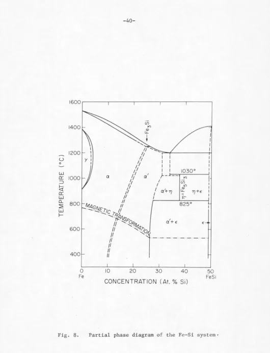
From the Fe-FeSi phase diagram in Fig. 8, the

intermetal-lie compound Fe

5si3(n) is in fact a high temperature phase,

0

stable only between 825 and 1030°C (22). This is unlike the

case for Mn

5si3 which is a congruently melted intermetallic com-( 22)

pound . A closer examination of the x-ray diffraction spectrum

of the Fe

5si3 compound indicates definite broadening of certain.low

angle lines, in particular, the (211) line shown with an arrow in Fig.

9b compared with the corresponding line in the Mn

5si3 diffraction

pat-tern in Fig. 9e. In Fig. 9c, the (211) line on the (Fe

(48)

6.90

---O<l:

..__..

0

I-z

<!

6.85

I-(J)

z

0

u

w

6.80

u

I-<!

_J

6.75

LJ_

0

20

40

60

80

100

Mn CONCENTRATION (

x)

IN (Fe

₁₀₀_x

Mn)

5

Si

3

Fig. 6. Lattice constant a _{of the (Fe 100_}xMnx)

5Si3 alloys. Filled circles (•) are

data reported in Ref. 20.

I VJ 00

(49)

u

~

z

~

(f)

z

0 4.76

u

w

u

~ ~ <t _J

4.72

0 20 40 60 80

Mn CONCENTRATION

(x)

IN (Fe

₁₀₀

_x Mnx)

₅

Si

3

100

Fig. 7. Lattice constant c of the (Fe

100_xMnx)5si3 alloys. Filled circles (•) are

data reported in Ref. 20.

I

w

(50)

u

0

w

1400

1200

0:: 1000

::J

~

0::

w

Q_

~ w

f--800

600

400

0 Fe

Fig. 8.

10 20 30 40

CONCENTRATION (At.% Si)

50 Fe Si

[image:50.554.8.538.31.723.2]

(51)

b

c

d

e

t

Fig. 9. Debye-Scherrer diffraction patterns of (a) (n

+

a1

) -Fe

67si33,

(b) n - Fe

5si3, (c) (Fe90Mn10) 5si3, (d) (Fe70Mn30) 5si3, and

(e) Mn

5Si3.

I

.i::--1--'

[image:51.784.135.768.23.532.2]

(52)

diffraction pattern exhibits a weaker but still noticeable broadening.

The (211) line broadening completely disappears in the (Fe

70Mn30)5si3

spectrum (Fig. 9d). This suggests that a second phase may exist even

in the quenched Fe-rich alloys. Figure 8 indicates that this second

phase might be either the a' or E: phase or a combination of both

a' and E •

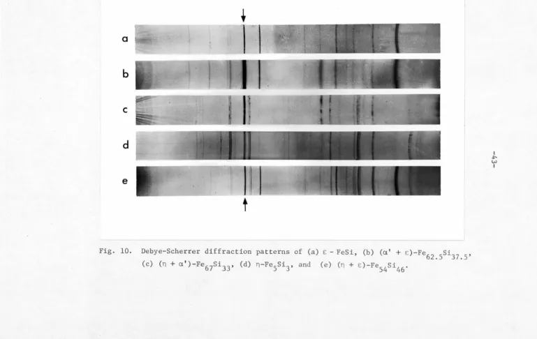
In order to identify the existing second phase, alloys of

Fe

67si33, Fe54si46 and FeSi were then made, which were annealed at 9S0°C for 10 days to form the (a' +

n), (n

+ E) and the E phases,

respectively. In addition, a two-phased (a' + E) alloy containing

37.S at.% Si was obtained by annealing a portion of the Fe

5si3 alloy at 7S0°c for 10 days. The prolonged-exposure (70 hrs) x-ray diffraction

technique, as described in Chapter II, was applied to all samples

concerned. These included the (a' + n)-Fe

67si33, (n + E:)-Fe54si46, £ -FeSi, (a'+E:)-Fe

62.5si37.5, n-Fe5si3, (Fe90Mn10)5si3, (Fe80Mn20)5Si3, (Fe

70Mn30)5si3,(Fe50Mn50)5si3 and Mn5si5 alloys. After reduction the diffraction patterns exhibit distinctive details of the lines as shown

in Figs. 9 and 10. These diffraction spectra indicate that at the

Bragg angle of (211) reflection, 28

=

70.026°, there co-exist a sharp

line in E:-FeSi diffraction pattern (Fig. lOa) and a much diffused line

in the (a' + E:)-Fe

62.5si37.5 spectrum (Fig. lOb). It is interesting to note that the corresponding line of particular interest is rather

sharp and narrow in the spectrum of (n + E:)-Fe

54si46 (Fig. lOe), while it is much more broadened in the case of (n + a')-Fe

67si33 (Fig. lOc). This leads one to believe that the diffused background of the (211)

line in the Fe

[image:52.553.24.550.41.749.2]

(53)

b

c

d

,i .. ,,., .. - - . ·-;·~.'

"' --.l~~ ,.. ;~.

~-,. '• ' ' '

·,.

>f., -;; !':x.~-.

f•-;

t

I

... ·~~

', c,.i ;9$

e

l

!{"f..~ \) . ·.~'j',...)-1''1'.

-,,

·..

..r;c~-• ._.

• i&i::

t

Fig. 10. Debye-Scherrer diffraction patterns of (a) E - FeSi, (b) (a'

+

E)-Fe

62.5si37.5, (c) (n

+

a')-Fe

67si33, (d) n-Fe5si3, and (e) (n

+

E)-Fe54si46.

I

+:-w

[image:53.785.0.770.50.536.2]

(54)

contribution of the small amount of the a' phase. The amount of the

a ' phase in Fe

5si3 was estimated as 10-20%. Furthermore, Fig. 9 shows

that the a' phase decreases as Mn concentration increases, and it

appears to vanish at composition x

=

30 .

Attempts were made to eliminate the a' phase in the Fe-rich

alloys. These included the prolonged annealing time up to a month,

the technique of solid state quenching, variation of annealing te

mpera-ture (between 825° and 1030°C), and introduction of 0.2- 0.5 at.%

carbon as the structure stabilizing agent(lB).

All of these efforts to stabilize the D8

8 structure in the

Fe-rich (Fe

100_xMnx)5si3 alloys were made in vain. One finally just

has to live with it.

B. Mossbauer Effect

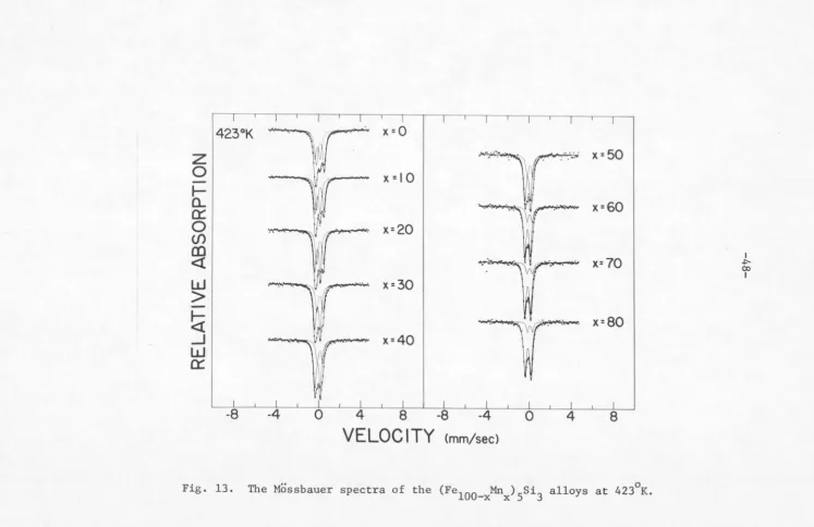
In Fig. 11, the room temperature Mossbauer absorption spectra

for the (Fe

100_xMnx)5si3 alloys are shown. All. alloys except for

x 0 and iO exhibit features of non-magnetic splitting. For

T 77°K and 423°K, the Mossbauer spectra of the alloys are shown,

respectively, in Figs. 12 and 13.

It is clear from these figures that all alloys are in the

para-magnetic state at T

=

423 K and, on the 0 other hand, all but fo1:

x

=

90 show magnetic hyperfine splitting at T

=

77°K. It can be seen

from Fig. 11 that as the Mn concentration x decreases from x

=

90 the spectrum deviates gradually from its symmetrical quadrupole

doublet. For higher Fe concentration, the appearance of a second

(55)

295°K

~-\.

,,,

"'~

r

,,,.,-

x

= O

y

x•50

I

51

~ • v ~ ,

I

\ 1

fM\/ \ . f

f

x = 10

_~

1

_1\_r-

x=GO

I-Cl..

~,

~

.

r-

x=25

I

---.;\

!

,..--

x= 70

en

m

<(

~I

WU

x=30

I

~

x=80

I

I +:--V1 I

~

T

x=40

_J

w

a:::

-8

-4

0

4

8 -8

-4

0

4

8

VELOCITY

<mm/sec>

Fig. 11. Mossbauer spectra of the (Fe

(56)

77°K

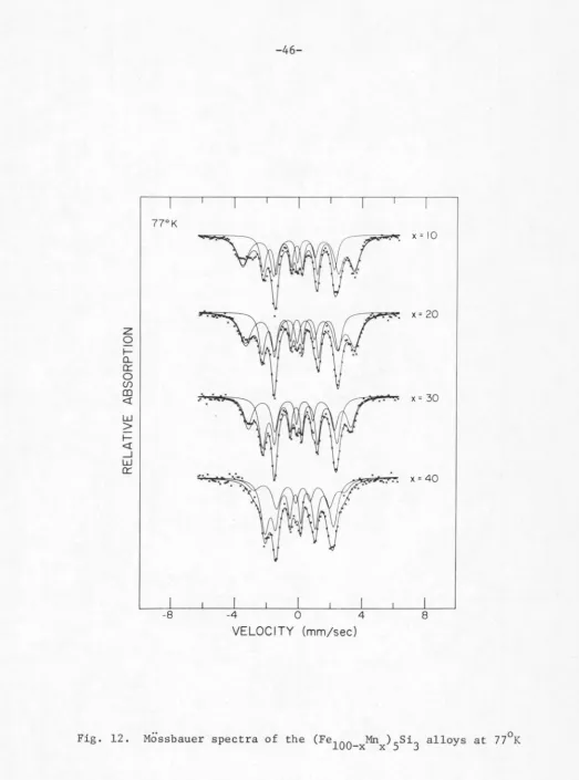
x = 10

.~

.

x= 20

z

0 1--CL

a:::

0

(/)

CD

x = 30 <! ,,.

w

>

1--<! _J

w

a:::

,.

..

x = 40

-8 -4 0 4 8

VELOCITY (mm/sec)

Fig. 12. Mossbauer spectra of the (Fe

[image:56.555.15.539.26.732.2]

(57)

z

0

l-o...

a::

0

(f)

CD

<I

w

>

1-<I

_J

w

a::

77°K

-8

x = 70

..

'\,

..

: x = 80

-4 0 4 ₈

VELOCITY (mm/sec)

Fig. 12 (continued). Mossbauer spectra of the (Fe

[image:57.552.9.538.32.738.2]

(58)

423°K

w

r

x =O

I

... ""' 17"!""' :··:: .• ·

x = 50

z

1

0

1

""

II

,-,

x =I 0

r-CL

1

0:::

1~11.V

I

.. ... . 'fV . ....

. ·•• '"""'~

,.

. ''"'

x=60

0

1

Cf)

II

.

.\ •. ~ ,...,... > • .

x=20

en

I

.·~.

,nr· ..

x=7o

I

<l

-I:'

00

· : c

0.iJ

...

I

w

>

.

8

.

I, ~

'

£ C W

.

F

x=30

>

-~

I

.

·~

W

/JI< ..

•::.· cJw,;: ~ ~ r;;::.-:• •."<• •·

x=80

x=40

w

0:::

-8

-4

0

4

8

-8

-4

0

4

8

VELOCITY

cmm/sec)

Fig. 13. The Mossbauer spectra of the (Fe

[image:58.774.15.762.30.514.2]

(59)

423°K

z

0

I- 295°K

CL

0::

0

(f)

CD

<[

w

>

I-<!

_J

77°K ,,.

..

w 'I.

...

0::

-8 -4 0 4 8

VELOCITY (mm/sec)

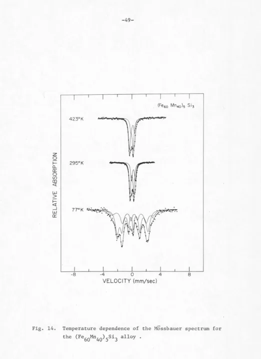
Fig. 14. Temperature dependence of the Mossbauer spectrum for

the (Fe

[image:59.561.17.539.30.747.2]

(60)

423°K "'""

.

...

z

295°K

0

I-0....

er:

0

(f) m <I w

>

77°K

t:r

_J

w

er:

..

...

'\,

4.2°K

,.

·.

-8 _-4 ₀ ₄ ₈

VELOCITY (mm/sec)

the (Fe

[image:60.556.16.544.23.739.2]

(61)

423°K

z

0

I-CL _295°K

0::

0 Cf)

CD <!

w

>

I-<! _J

77°K

w

...

.

0::

-8 -4 0 4 8

VELOCITY (mm/sec)

the (Fe

[image:61.555.11.540.24.743.2]

(62)

Mossbauer spectra as functions of temperature for the alloys

(Fe

60Mn40)5si3, (Fe50Mn50)5Si3 and (Fe40Mn60)5Si3, respectively.

As the results of Mossbauer effect are known to reflect the

structural environment of the isotope, the crystal structure and its

symmetry described in part A of this chapter can provide a certain.

guide to the fitting of the Mossbauer spectrum. The fact that Fe

atoms occupy two inequivalent sites suggests that a two-site approx

i-mation might be adopted as a fitting scheme. This means that the

observed absorption spectrum may be analyzed as the superposition of

two components contributed from Fe

1 and Fe11 Since the Fe atoms

in a hexagonal lattice have lower than a three-fold symmetry, it would

be reasonable in general to expect the existence of a quadrupole

splitting.

The Mossbauer absorption spectra were analyzed through the use

of a computer programC44) which least-squares fits the data points to

the theoretical function with respect to the type of interaction. The

line shape was assumed to be Lorentzian. As can be seen in Figs.

11-16, generally all spectra were fitted reasonably well with two

sites. However, fitting the outer peaks of the Fe

5si3 spectra at 77°K

and 295°K seems to present some difficulty, and this appears to become

less serious in the case of (Fe

90Mn10)5Si3 spectra.

1. Room Temperature Results

Magnetic hyperfine splittings combined with quadrupole inte

rac-tions have been observed in alloys for x

=

0 and 10 (Fig. 11). In

particular, the room temperature spectrum of (Fe

80Mn20)5si3 appears to

(63)

not low enough for the spectrum to show well resolved hyperfine spl it

-tings. The fact that only electric quadrupole splittings are present

in alloys for x

=

25,30,40,··· ,90 indicates that their magnetic tra

n-0

sition temperatures are below 295 K.

The Fe

5si3 Mossbauer spectrum consists of two different hy

per-fine splittings (hfs). The ratio of the area under the larger hfs to

that of the smaller one is 6:4. In view of the fact that absorption

intensities are directly proportional to the number of Fe atoms in

sites, it is easy to correlate the contribution from Fe

1 with the

larger isomer shift corresponding to the larger hfs, and the contri

bu-tion from Fe

11 with the smaller isomer shift. Since the isomer shift

is usually a smoothly varying function of alloy composition, the co

n-tribution from the two different sites may be easily distinguished with

the aid of their isomer shifts which in the present case are appre

-ciably different.

The computer-analyzed parameters of the room temperature

Mossbauer spectra are tabulated in Table II. Isomer shift and q

uadru-pole splitting are plotted against Mn concentration in Figs. 17 and

18, respectively. It is particularly interesting to note the

composi-tional variation of the relative intensity which at first increases

slowly until the composition x

=

50 where it begins to increase

exponentially as shown in Fig. 19. This immediately suggests a prefe

r-ential substitution between Fe and Mn atoms (i.e., Fe

1 by Mn atoms

or Mn

(64)

Computer analyzed Mossbauer parameters measured at T

=

29S°K

o(mm/sec) 6Eq (mm/ sec) t1ii£( kOe)

.W or W

0

Composition Site _Intensity _(mm/_se_c) _a

FeSSi

3 I .92 ± .004 -.470 ± .007 lSS.9 ±-3 .7S7 ±-008 . 241 ±. 018 1.006 ± .127 II -.037 ±.001 .206 ±.003 89. 2 ± .1

.sos

±.OOS .373 ±.014 . 240 ±. 021

(Fe90MnlO)SSi3 I .194 ± .004 -. 320 ±. 007 148.1±.3 . 708 ±. 019 . 249 ±. 022 .827 ± .125 II -.037 ± .003 .141 ±.OOS 93.2±.2 .453 ±.01S . 268 ± • 01S . 231 ± • 066 (Fe7SMn2S)SSi3 I . 212 ±. 001 . 633 ± • 002 . 479 ±. 004 . 283 ±. 007

II -.022 ± .001 .519 ± .001 .S90 ±.004 . 283 ±. 002 (Fe70Mn30)SSi3 I . 212 ± .001 • S94 ±. 002 . 414 ±. 003 . 266 ±. 002

I I -.020 ± .001 . Sl9 ±. 001 • S60 ±. 004 .266 ± .002 I

V1 (Fe60Mn40)5Si3 I . 203 ± .002 . S40 ±. 002 .407 ±.002 .279 ± .003 +' I

I I -.017 ± .001 .S23 ±.001 . 677 ± .006 .279 ±.003

(Feso.t-Inso) s 5 i3 I .197 ±.001 . Sl2 ±. 001 .383 ± .003 .317 ±.002 II -.023 ±.001 .Sl7 ±.001 .73S ±.004 .317 ± .002 (Fe40Mn60)SSi3 I .193 ±.004 .404 ±

.oos

.242 ±.008 .261 ±.003

I I -.01S ±.001 .S31 ±.001 .868 ± .011 .261 ±.003

(Fe30Mn70)SSi3 I . 202 ±.

oos

.493 ± .008 .194 ± .009 . 2S4 ±. 003

I I -.Oll ± .001 • SS2 ±. 001 .914 ± .012 .2S4 ±.003

(Fe20Mn80)SSi3 I .197 ±.013 . S31 ±.017 .106 ±.013 • 2SS ± . 004

I I -.006 ± .001 .S63 ±.002 . 944 ±. 017 . 2SS ± . 004

(Fe10Mn9o)ssi3 I . 211 ±. 016 .S91 ±.024 . 068 ±. 010 . 24S ± . 003

(65)

Q)

~

E

0.2

E

... I-lJ....

0.1

-I

(/)

n:

w

0.0

~

0

(/)

-

-0.I

SITE

I

-.c:>-1), a

~ •=•o·----24iWlitO a -O o

•

0

SITE II

-

..

20

40

60

80

Mn CONCENTRATION (x)

IN (Fe

100

_x

Mn

x )

5

Si

3

100

Fig. 17. Composition dependence of the isomer shift at room temperature.

I

V1 V1

Lattice anomalies and magnetic states in Fe 5Si 3 Mn 5Si 3 alloys

ACKNOWLEDGEMENT

ABSTRACT

TABLE OF CONTENTS

SINGLE CHANNEL AMPLIFIER ANALYZER

III. BRIEF REVIEW OF RELEVANT THEORIES

IV. EXPERIMENTAL RESULTS AND DATA ANALYSIS

0R Mnrr AT Z = 1/4 AND 3/4

0

0

0

Mn CONCENTRATION (

• i&i::

0

0

VELOCITY

0

0

0

0

0

0

SITE II