Stochastic Partial Differential Equations
Thesis by Mulin Cheng
In Partial Fulfillment of the Requirements for the Degree of
Doctor of Philosophy
California Institute of Technology Pasadena, California
2013
c
To my wife
Lu Chi,
and my parents
Acknowledgements
I owe my deepest gratitude to my adviser Prof. Thomas Y. Hou. Without his constant inspirations, encouragements, and challenges, I would not have had the chance to complete this thesis in the present form. A discussion from 10 a.m. to 2 a.m. not only marked the turning point in my research, but also enlightened and will continue to enlighten me throughout my future career and life.
Besides my adviser, I would like to thank the rest of thesis committee — Professor Houman Owhadi, Daniel I. Meiron, and James L. Beck — for taking time to review and comment on my thesis. I would also like to thank the staff of ACM department — Sydney Gastang, Carmen Nemer-Sirois, William Yardley, and Sheila Shull — for their help over the past years.
In addition, I would like to thank Prof. Yalchin Efendiev and Dr. Xiaohui Wu for their hospitality and many inspiring discussions when I visited them. My sincere thanks also go to Prof. Lexing Ying, for help and endless suggestions on living and research when he was a postdoc here.
I am grateful to Dr. Pengchong Yan, Dr. Zuoqiang Shi, and Dr. Zhiwen Zhang for many stim-ulating discussions over the past three years. I thank my friends at Caltech — Maolin Ci, Xin Hu, Peyman Tavallali, Wuan Luo, Lei Zhang, Guo Luo, Chia-Chieh Chu, Zhen Li, Yuebin Liu, Yao Sha, Yan Xia, Stephen Becker, Catherine Beni, Yaniv Plan and Svitlana Vyetrenko — for the help, the fun, and the good time we had together.
and how much I love you.
Abstract
Contents
Acknowledgements iv
Abstract vi
1 Introduction 1
1.1 Uncertainty Quantification and Stochastic Partial Differential Equations . . . 2
1.2 Existing Numerical Methods . . . 4
1.2.1 Non-Sampling Methods . . . 4
1.2.2 Non-Intrusive Sampling Methods . . . 5
1.2.3 Intrusive Methods . . . 7
1.2.4 Post-Processing. . . 9
1.3 Exploring Sparsity . . . 10
1.3.1 Karhunen-Loeve Expansions . . . 11
1.3.2 Overview of Dynamically Bi-Orthogonal Methods . . . 15
1.4 Summary of the Thesis . . . 17
1.4.1 Summary of Main Contributions . . . 18
1.4.2 Roadmap . . . 20
2.1.1 Derivations of Reduced-Order Model for Truncated KLE . . . 25
2.1.2 Enforcing Bi-Orthogonality Condition. . . 27
2.1.3 Eliminating Time Derivatives from RHS. . . 29
2.1.4 DyBO Formulation for Time-Evolutionary SPDE . . . 33
2.2 Bi-Orthogonality Preservation . . . 35
2.3 Representation of Stochastic Modes . . . 40
2.3.1 Ensemble Representation. . . 40
2.3.2 Spectral Representation . . . 41
2.3.2.1 Some Preliminaries of gPC Methods . . . 41
2.3.2.2 gPC Version of DyBO . . . 44
2.3.3 gSC Version of DyBO . . . 46
2.4 Eigenvalue Crossing . . . 47
2.4.1 Detection of Eigenvalue Crossing . . . 48
2.4.2 FreezeYorY-Stage . . . 48
2.4.3 FreezeUorU-Stage . . . 52
2.5 Error Analysis . . . 56
2.5.1 Type-0Errors . . . 56
2.5.2 Type-JError . . . 60
2.5.3 Type-KL Error . . . 62
2.6 Adding or Removing Mode Pairs . . . 64
2.6.1 Removing Modes. . . 64
2.6.2 Adding Modes . . . 65
2.7 Overall DyBO-gPC Algorithm . . . 71
2.7.2 DyBO-gPC Algorithm . . . 72
3 Applications to Spatially One-dimensional SPDEs 73 3.1 SPDE Purely Driven by Stochastic Force. . . 74
3.1.1 Eigenvalue Crossing . . . 78
3.1.2 Adding and Removing Modes . . . 79
3.2 Linear Deterministic Differential Operators with Random Initial Conditions . . . . 82
3.3 Burgers’ Equation Driven by Stochastic Forces . . . 85
3.3.1 gPC Formulation for Stochastic Burgers’ Equation . . . 86
3.3.2 DyBO-gPC Formulation for Stochastic Burgers’ Equation . . . 89
3.3.3 Numerical Examples . . . 93
3.3.3.1 Hierarchy of Errors . . . 95
3.3.3.2 Numerical Results . . . 97
4 Applications to Spatially Two-Dimensional SPDE 102 4.1 Computational Complexity Analysis . . . 102
4.1.1 Storage Complexity . . . 103
4.1.2 Computational Cost . . . 104
4.1.2.1 Linear PDE Driven by Stochastic Forces . . . 105
4.1.2.2 Second-Order Nonlinear PDE Driven by Stochastic Forces . . . 107
4.2 Stochastic Navier-Stokes Equations . . . 110
4.2.1 gPC and DyBO-gPC Formulations of SNSE. . . 113
4.2.2 Numerical Results . . . 114
5.2 Generalized KLE forL2 Ω→ Hk(D) . . . 129
5.3 Generalized DyBO forL2 Ω→ Hk(D) . . . 134
6 Generalizations of DyBO for a System of Time-Dependent SPDEs 136 6.1 DyBO for a System of SPDEs . . . 137
6.2 Stochastic Navier-Stokes Equations with Boussinesq Approximation . . . 140
6.2.1 gPC Formulation of SNSE . . . 143
6.2.2 DyBO Formulation of SNSE . . . 144
6.3 Numerical Results. . . 145
6.4 Parallelization . . . 147
6.4.1 Parallelization Strategy . . . 151
6.4.2 Implementation and Speedup. . . 153
7 Generalized Stochastic Collocation Formulation of DyBO Method (DyBO-gSC) 155 7.1 Formulation and Algorithm . . . 155
7.1.1 Sparse Grid . . . 156
7.1.2 Generalized Stochastic Collocation Method (gSC) . . . 157
7.1.3 gSC version of DyBO Method (DyBO-gSC) . . . 159
7.2 Numerical Example — Stochastic Burgers Equation. . . 161
8 Conclusions and Future Work 164
A Derivation of the gPC formulation of Time-Evolutionary SPDE 170
B Proof of Corollary 2.8 and 2.9 172
D Derivations of gPC Formulation of SNSE 181
E Derivations of the DyBO Formulation of SNSE 186
List of Figures
1.1 Conceptual illustration of efficiency of gPC, gSC, MC, and CM with respect to
di-mensionality of random space . . . 9
1.2 The numerical simulation process of SPDEs . . . 10
2.1 Illustration of eigenvalue crossing and two strategies,Y-Stage andU-Stage . . . 47
2.2 Illustration of strategies of adding and removing mode pairs . . . 69
3.1 Mean and STD computed by DyBO at timet= 1.2 . . . 79
3.2 Spatial modes in KL expansion of SPDE solution computed by DyBO at timet= 1.2 79 3.3 Eigenvalues computed by DyBO. Two zooming-outs are provided at the time when two eigenvalues cross each other to show the invocation ofU-stage Algorithm 2.2 . 80 3.4 Bi-orthogonality of spatial and stochastic modes. Orthogonality ofU is preserved throughout the computation while stochastic modes deviate from orthogonality only at eigenvalue crossing . . . 80
3.5 Eigenvalues. Eigenvalues are plotted as function of time. λ3 becomes small near t= 0.25 . . . 81
3.6 Change rate of the largest unresolved eigenvalue d √ λ3 dt . Solid line is given by the exact solution, while the dotted line are computed as described in Sec. 2.6.2 . . . 82
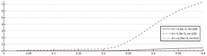
3.8 Spatial modes in KL expansion of SPDE solution computed by DyBO at timet= 0.4 85 3.9 L2relative errors of STD computed by DyBO with different spatial and temporal grid
sizes. The horizontal axis is timet . . . 85
3.10 Hierarchy of solutions . . . 97
3.11 L2relative errors of mean and STD as functions of time . . . 99
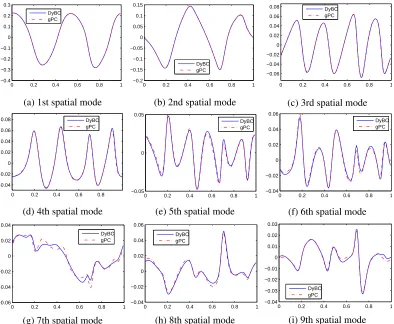
3.12 The first nine spatial modes computed by DyBO at timet= 1.0 . . . 100
3.13 Stochastic modesHAcomputed by DyBO at timet= 1.0 . . . 101
4.1 Stochastic flows driven by stochastic forcef in 2D unit square . . . 113
4.2 Wall time of a single RK step of the DyBO-gPC system as a function ofm . . . 117
4.3 Mean and STD of vorticity field at timet = 1.0. The left column is computed by DyBO-gPC, while the right column is computed by gPC. They are essentially the same.118 4.4 The first four spatial modes at timet= 1.0. The left column is computed by DyBO-gPC, while the right column is computed by gPC. They are essentially the same. . . 119
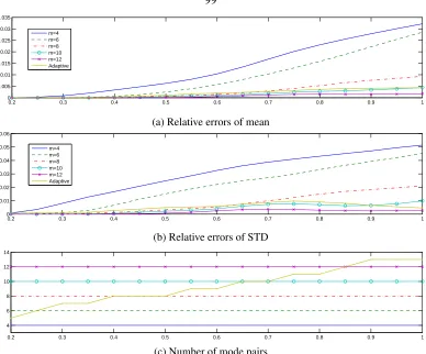
4.5 The L2 relative errors of mean and STD of vorticity field computed by DyBO. The errors are plotted as functions of time in the top two figures, while the numbers of mode pairs used in the adaptive strategy are given in the last figure. . . 120
4.6 Comparison of energy spectrum of gPC and DyBO solutions at timet= 1.0. . . 122
4.7 Comparisons of gPC and DyBO methods . . . 124
6.1 Stochastic flow driven by stochastic force and buoyancy force due to Boussinesq
approximation. On the left: Diagram of the stochastic flow in an unit square. The
gravity is downward parallel toy-axis and periodic boundary conditions are assumed
on bothxandydirections. On the right, the initial temperature field is plotted, while
the initial vorticity is uniformly zero. . . 140 6.2 STD of vorticity and temperature fields at timet = 1.0. Left column by DyBO and
right column by gPC . . . 148 6.3 Vorticity spatial modes at timet = 1.0. Left column by DyBO and right column by
gPC . . . 149 6.4 Temperature spatial modes at timet= 1.0. Left column by DyBO and right column
by gPC . . . 150 6.5 L2relative errors of vorticity and temperature STDs as functions of time. The
evolu-tions of the numbers of vorticity and temperature mode pairs are also given in the last
figure. . . 151 6.6 Illustration of spatial domain decomposition . . . 152
List of Tables
1.1 Illustration of the exponential growth of the number of polynomial chaos basis
func-tions,NP. . . 8
3.1 Relative errors of statistical quantities computed by DyBO, Adaptive-DyBO, and gPC
at timet= 1.0 . . . 100
4.1 Storage complexity comparison between gPC and DyBO-gPC methods . . . 104 4.2 The computational time of some typical terms on the right-hand side of the
DyBO-gPC formulation . . . 106 4.3 The computational time of terms on the right-hand sides in the gPC formulation for
second-order nonlinear PDE driven by stochastic forces. . . 108 4.4 The computational costs of matrix-tensorAandT(H)products . . . 109 4.5 The computational costs of terms on the right-hand sides in the DyBO-gPC
4.6 Comparison of wall times of a single RK step of gPC and DyBO-gPC systems.
De-pending on whether the sparsity of tensorT(H)is explored or not, the wall times are
reported in the second and third columns for gPC method, respectively. The wall
times of DyBO-gPC are reported in columns 4–7 for m = 4,8,12,16. The
expo-nentsαandβin eqn. (4.9) are estimated by linear regression. The last column in red
uses wall times corresponding tom= 8,12,16to compute the exponentα, while the
second to last column in gray uses all four values of mto estimate the exponentβ.
The values ofβare reported in the last two rows. . . 116
6.1 Speedups by proposed parallelization strategy for different spatial grids and mode
number vectors. Wall times of a single RK time step for different parameters are
given in the second, fourth, sixth, and eighth columns. All times are in seconds. . . . 154
List of Algorithms
2.1 Strategy inY-Stage . . . 51
2.2 Strategy inU-Stage . . . 55
2.3 Removing Mode Pairs . . . 65
2.4 Adding Mode Pairs . . . 70
Chapter 1
Introduction
Uncertainty arises in many complex real-world problems of physical and engineering interests, such as wave, heat, and pollution propagation through random media [75], and flow driven by stochastic forces [109,85,73,108,55,53]. Additional examples can be found extensively in other branches of science and engineering, such as geosciences [90,32], statistical mechanics, meteorology [28], biology [11], finance [42,43], and social science [64]. Meanwhile, Ordinary Differential Equations (ODEs) and Partial Differential Equations (PDEs) are often, if not all the time, adopted to describe and represent physical, engineering, economic or even social models. Therefore, Stochastic Ordi-nary Differential Equations (SODEs) and Stochastic Partial Differential Equations (SPDEs), which contain randomnesses in terms of random variables or stochastic processes, are natural extensions of ODEs and PDEs to investigate Uncertainty Quantification (UQ).
1.1
Uncertainty Quantification and Stochastic Partial Differential
Equa-tions
There are a number of different sources of uncertainty in SPDEs. Below we will discuss a few of them which have been used widely in the literature [62,85,27].
Parametric Uncertainty which comes from some model parameters whose exact values are infeasible to obtain in practice. A non-trivial example comes from predictions of flow and transport in natural porous media such as water aquifer and oil reservoirs [75], which essentially requires numerical simulations of an elliptic PDE for the steady state flowu,
− ∂
∂xp
apq(x, ω) ∂
∂xqu(x, ω)
=f(x),
where the permeability fielda(x, ω)contains random model parameters in the sense that their exact values are infeasible to obtained in practice primarily due to low resolution of seismic data.
Model deficiency/inadequacywhich comes from discrepancy between mathematical models and physical processes. Such discrepancy may be due to the lack of full understanding of true physical processes, or the lack of sophisticated mathematical tools available to describe adequately the underlying complex physical processes, or simplifications of complicated mathematical models for further theoretical or numerical analysis. A concrete example, which we will discuss extensively in the thesis, is randomly forced Burgers or Navier-Stokes equations. The large-scale structures of flows are primarily governed by deterministic PDEs and random forcingf(x, t, ω) in terms of random variables or Brownian motions are introduced to model unresolved small-scale effects from turbulence.
of modern computer architectures and numerical approximation errors arising from discretizations, numerical integrations, and truncation of infinite summations. Generally, such numerical algorithms solve exactly some modified ODEs/PDEs, which are similar to the original ODEs/PDEs with extra terms. However, the exact forms of such terms are only known in very limited applications, so it is convenient to introduce noise terms to replace them and to study the effect of numerical errors on complicated systems.
Analytical solutions of SODEs/SPDEs are only available in very special cases. For most of practical problems, numerical schemes are used to approximate stochastic solutions and quantify uncertainty. However, due to the complex nature of SODEs and especially SPDEs, numerical simu-lations pose a great challenge to the applied mathematical community. In this thesis, we are primar-ily concerned with SPDEs and their efficient numerical schemes. Methods developed in this thesis are still applicable to certain types of SODEs.
Throughout the thesis, we consider the following time-evolutionary/time-dependent stochastic partial differential equation
∂u
∂t(x, t, ω) =Lu(x, t, ω), x∈ D ⊂R
d, t∈[0, T], ω∈Ω, (1.1a)
u(x,0, ω) =u0(x, ω), (1.1b)
B(u(x, t, ω),∂u
∂x(x, t, ω)) = 0, x∈∂D, (1.1c)
1.2
Existing Numerical Methods
Before embracing the data-driven philosophy underlying in this thesis, it is worth reviewing briefly existing numerical methods for SPDEs along with their applicable regime and limitations.
1.2.1 Non-Sampling Methods
Perturbation methods (PM). When both input and output uncertainties are small compared to mean values, perturbation methods are shown to be effective in many engineering problems [75]. These methods start with expanding stochastic solutions via Taylor expansion and result in a system of deterministic equations by truncating after certain order. Typically, at most second-order expan-sions are used in practice as the system of equations become very cumbersome if higher-order terms are included. One limitation of perturbation methods is that the magnitude of the uncertainty must be small. Moreover, they do not reveal faithfully probability distributions of stochastic solutions.
Probability Density Function Methods (PDF) and Moment Equation (ME) Methods.When statistical information is of main interests, instead of tackling directly SPDEs, effective equations for moments and PDFs can be derived and solved numerically, such as Fokker-Planck equations [68]. For nonlinear problems, such methods suffer from closure issues, i.e., equations of lower moments depend on higher-order moments or certain terms in PDF equations take complicated integral forms and are hardly computable. Such difficulty can be alleviated by using some heuristic arguments to achieve closure, but it also introduces modeling errors which are hard to control.
single input can only cause small oscillation on outputs, i.e., response functions are well centered around their expectations. Such a phenomenon is called concentration of measure. Study of this phenomenon can be tracked back to Levy and has been studied systematically by Milman, Ledoux [74], Talagand [105], etc. A bunch of powerful concentration-of-measure inequalities, such as McDiarmid’s inequality, have been developed in the past years, which can be used to provide tight bounds on response fluctuations over means. Owhadi and others have demonstrated the success of this method in the context of parameter sensitivity and certification [2, 3, 107, 104, 76], i.e., showing the failure probability of complex system is within a certain tolerance, and have proposed the Optimal Uncertainty Quantification (OUQ) framework [103, 92] to achieve optimal bounds on uncertainty for a given set of assumptions and information. However, these methods do not reveal the KL expansions of the stochastic solutions, which is important for understanding physical systems.
1.2.2 Non-Intrusive Sampling Methods
Modern software systems for numerical simulations of deterministic models of engineering or phys-ical systems can be very complex and may contain more than thousands of lines of codes and its validations against experimental results may take years. For example, sophisticated Computational Fluid Dynamic (CFD) code can easily exceed ten thousands of line of codes [89]. Changes in a small segment of code may introduce unforeseeable bugs and require another round of validations. Therefore, sampling methods are preferred in some of industrial applications for their non-intrusive nature, i.e., requiring no direct modifications on legacy codes.
Monte Carlo Method (MC).Because of stability and non-intrusive nature of MC, it remains a popular numerical method for SPDEs especially when the dimensionality of input uncertainty,
OM−12
, where M is the number of realizations, so MC methods are “famous” for their slow convergence.
Quasi-Monte Carlo Method (qMC). The slow convergence of MC is partially due to the low uniformity or high discrepancy of pseudo-random number sequences generated by computer algo-rithms [60,59,83,17]. qMC methods [45,84] use instead a deterministic sequence of numbers of low discrepancy to achieve almostO M−1
for small to moderate dimensionality of input uncer-tainty. However, such convergence rate is still considered to be slow for industrial-scale applications where numerical simulation of a single realization may take hours or even days. Furthermore, the above convergence rate degrades toOM−12
for largep.
Generalized Stochastic Collocation Method (gSC). gSC [78,87,33,7,106,116, 7] meth-ods explore the smoothness of stochastic solutions with respect to random variables, and use in-stead a deterministic sequence of sampling points{ωi}Mi=1 resulting from tensor products of one-dimensional quadrature points. The exact locations of such points and weightswi associated with them depend on underlying probability distributions. Because of tensor products, the number of sampling points increases exponentially fast as the number of random variables increases, which is also known ascurse of dimensionality. Sparse grid [18] is introduced and further exploits smooth-ness to reduce the number of sampling points to some extent.
The sampling methods are after an ensemble of solutions {u(x, ωi)}Mi=1 along with weights {wi}Mi=1 associated with each realization. The above mentioned three non-intrusive methods only differ in the selection of sampling points and associated weights.
aspects of numerical simulations of SODEs and SPDEs to achieve accelerations. One is that, besides sampling errors, numerical errors due to spatial and temporal discretizations also contribute to final results and thus the effective number of sampling points are constrained by grid resolutions. The other, which may be more important, is that the variances of solution differences on two adjacent discretization grids in a geometrical grid hierarchy may decay exponentially fast and the number of sampling points on each level decay exponentially. An intrinsic limitation associated with MLMC methods comes from that the fore-mentioned assumption about variance decay is true only when the grid size reaches some asymptotic regime. In this case, each realization on the “coarse level” is already quite expensive and the computational saving is not as much as one would like to get.
1.2.3 Intrusive Methods
Generalized Polynomial Chaos Methods (gPC). While non-intrusive sampling methods repre-sent the solution of SPDEs as an ensemble of realizations, another way to reprerepre-sent stochastic solutions is to employ truncated expansion on a set of polynomial chaos basis and drive a sys-tem of coupled deterministic PDEs. The stochastic solution generally takes the form ofu(x,ξ) = P
α∈Juα(x)Hα(ξ)whereJis some multi-index set and will be explained in detail in Sec.2.3.2.1.
meth-ods also suffer from the curse of dimensionality. For example, if a SPDE involvep independent random variables and only polynomials of total order at mostP are chosen, then the total number of polynomial chaos basis functions is
NP =
P +p p
= (P +p)!
P!p! ,
which increases exponentially and can easily exceed available computational resource even for small
pandP as demonstrated in Table1.1.
p P NP
4 3 35
4 5 126
6 3 84
6 5 462
8 3 162
8 5 1287
[image:26.612.282.365.274.397.2]10 5 3003
Table 1.1: Illustration of the exponential growth of the number of polynomial chaos basis functions,
NP.
gPC or gSC
CM
MC
Efficiency
Dimensionality of random space
[image:27.612.150.498.69.191.2]gPC or gSC Applicable ??? CM Applicable
Figure 1.1: Conceptual illustration of efficiency of gPC, gSC, MC, and CM with respect to dimen-sionality of random space
1.2.4 Post-Processing
The efficiency of MC, gPC, gSC, and CM with increasing number of random variables are illustrated in Fig.1.1. Both gPC and gSC suffer from the curse of dimensionality, so their efficiencies degrade very fast as the number of random variables increases. On the other hand, concentration-of-measure inequalities, although powerful, inherently assume the presence of a large number of uncertainty sources and therefore are only effective at the high end of random dimensions. The convergence rate of MC methods depends largely on the number of realizations, so its efficiency remains almost constant, regardless of the dimensionality of the space of random variables. It is clear that other structures of stochastic solutions of SPDEs should be further explored to design new and more efficient numerical algorithms.
One of potential candidates reveals itself after we pay a close examination to the post-processing of intrusive and non-intrusive methods, an aspect which receives a little attention in the litera-ture. The numerical simulation process of SPDEs never stops at just getting a set of realizations {u(x, ωi}Mi=1for non-intrusive methods or a set of gPC coefficients{uα(x)}α∈Jfor intrusive
Solution Process ∂u
∂t(x, t, ω) =Lu(x, t, ω)
Post-process KL Expansion Or
Monte Carlo Solution
gPC Solution
Or u≈u¯+Pmi=1ui(x, t)Yi(ω, t)
SPDE
gSC Solution
Dynamically Bi-Orthogonal Method (DyBO)
Figure 1.2: The numerical simulation process of SPDEs
The Karhunen-Loeve Expansion (KLE) has received increasing attention in many fields, such as statistics [1], image processing [65], and UQ [100, 22]. Among many reasons for its popular-ity, one is that KLE reveals not only mean and variance but also the most important spatial and stochastic modes of the stochastic solution, allowing sparse representation of stochastic solutions and extractions of physical understandings. However, the computation of KLE is not trivial at all. For example, the computation of KLE from an ensemble of realizations generally involves solving a large-scale SVD problem. Certain methods have been developed to make such computation more efficient, e.g., randomized algorithms [86]. If we look at the entire numerical simulation process of SPDEs in Fig.1.2, we find that a large number of realizations or gPC coefficients arefirstobtained after a lot of computational resources and time are spent, and then“condensed”to KLE. Therefore, a question arises naturally,
Can we skip the step of solving a large number of realizations or gPC coefficients and
target directly KL expansions of SPDE solutions?
1.3
Exploring Sparsity
method for the numerical simulation of SPDEs, which fully explores the sparsity in the sense of KL expansions. To make the following discussion more precise, we first review briefly KL expansions in this section and then outline the philosophy of proposed data-driven algorithms for SPDEs. Before that, the following two remarks are worth mentioning.
Remark1.1. The sparsity which we explore here is not the usualentry-wise sparsity, i.e., only a few non-zero entries or coefficients, butdata-sparsity, i.e., few data are required to provide an accurate description of the stochastic solutions. Such a difference has been pointed out by Hackbusch [47], and Hackbusch and Khoromskij [48], in the context of matrices. For numerical SPDEs, the former sparsity has been explored in elliptic PDEs with stochastic coefficients by Todor and Schwab [106], Bieri and Schwab [14], Schwab and Todor [99], and Doostan and Owhadi [29]. However, the set of sparse coefficients are unknowna priori, which is necessary for effective computation reduc-tion. A heuristic algorithm based on purely-stochastic problems is suggested by Schwab to select such a set prior to computations. Doostan formulatesl0- and l1- optimization problems and uses Orthogonal Marching Pursuit (OMP) algorithm and Spectral Projected Gradient (SPGL) algorithm to demonstrate its effectiveness.
Remark1.2. The combined sparsity, i.e., data sparsity and entry-wise sparsity, has been explored
by Chandrasekaran et al. [24,23] in the context of matrix decomposition. However, it is not clear at the moment how such combined structures should be explored in numerical SPDEs.
1.3.1 Karhunen-Loeve Expansions
Consider a probability space(Ω,F,P), whereΩis called the event space and is equipped with aσ
spatial domainD ⊂Rdis a second-order stochastic process, i.e.,
u∈L2(D ×Ω) =
v(x, ω)| Z
D
Z
Ω
v(x, ω)2P( dω) dx
.
Sometimes, we also writeL2(D ×Ω) =L2 Ω→L2(D)to emphasize thatuis a function-valued
random variable taking values inL2(D). HereL2(D)is the Hilbert space equipped with the usual
inner product
hf(x), g(x)i
L2(D)= Z
D
f(x)g(x) dx,
which induces the usualL2-norm
kf(x)k2
L2(D)=hf(x), f(x)i
onL2(D)and a norm
kv(x, ω)k2
L2(D×Ω)=
Z
D
Z
Ω
v(x, ω)2P( dω) dx=E
h
kv(x, ω)k2
L2(D)
i
onL2(D ×Ω). When no ambiguity arises, we may drop subscripts. Denoteu¯(x) = E[u(x, ω)],
the expectation ofu, and the covariance function of stochastic processuis defined as
Covu(x, y) =E[(u(x, ω)−u¯(x)) (u(y, ω)−u¯(y))], ∀x, y∈ D.
When no ambiguity arises, we simply writeCov(x, y). The covariance function naturally defines a linear operator onL2(D), i.e.,
g(x) = Z
D
It is easy to show that this linear operator is compact, self-adjoint and positive definite and, by Mercer’s theorem, admits a spectral decomposition [41] onL2(D),
Cov(x, y) =
∞
X
i=1
λifi(x)fi(y),
whereλi’s andfi’s are the eigenvalues and eigenfunctions of the covariance kernel and{fi(x)}∞i ⊂
L2(D)form a complete orthonormal basis, i.e.,hfi, fji=δij. The stochastic processu(x, ω)can
be expanded in a Fourier-type series as
u(x, ω) = ¯u(x) +
∞
X
i=1 p
λifi(x)Yi(ω), (1.2)
where random variablesYi(ω)’s are zero mean and uncorrelated, i.e.,E[Yi] = 0, E[YiYj] = δij,
and are given by
Yi(ω) =
1 √
λi
Z ˜
u(x, ω)fi(x) dx, fori= 1,2,3,· · · ,
withu˜(x, ω) =u(x, ω)−u¯(x).fi(x)’s or√λifi(x)’s are referred to as spatial modes andYi’s are referred to as stochastic modes in this thesis.
The KL expansion (1.2) is named after Kari Karhunen and Michel Loeve who derived it in-dependently around 1947 [41]. Generally, the eigenvaluesλi’s are sorted in descending order and
cluster at zero, whose decay rate depends only on the regularity of the covariance kernelCovu.
It has been shown that algebraic decay rate, i.e.,λi = O (i−γ), is achieved asymptotically if the covariance kernel is of finite Sobolev regularity, and exponential decay rate, i.e., λi = O e−γi
, if the covariance kernel is piecewisely analytical [100]. In either case, anm-term truncated KLE converges to the original stochastic processu(x, ω)ink·k
computing the truncation error
kmk2L2(D×Ω) =
∞
X
i=m+1 p
λifi(x)Yi(ω)
2
L2(D×Ω) =
∞
X
i=m+1
λi →0, asm→ ∞,
where we have used the bi-orthogonality of KLE.
The most important property characterizing KLE is the so-called error-minimizing property, which can be summarized in the following theorem,
Theorem 1.1 (Error Minimizing Property of KLE). Among all complete orthonormal bases of
L2(D), KLE of second-order stochastic processu(x, ω)∈L2(D ×Ω)minimizes them-term
trun-cation errors form= 1,2,3,· · ·, i.e.,
{fi(x)}∞i=1 = arg minhhi, hji=δijkm(x, ω)kL2(D×Ω), (1.3)
where them-term truncation error
m(x, ω) =u(x, ω)−u¯(x)− m
X
i=1 p
θihi(x)Zi(ω),
andZi(ω) = √1 θi
R ˜
u(x, ω)hi(x) dx.
Proof. See [41] or Sec.5.2.
While the error-minimizing property implies KLE is the sparsest expansion of a second-order stochastic process in the energy normk·k
L2(D×Ω), bi-orthogonality of KLE characterizes it
com-pletely from another aspect, i.e.,
admits a unique bi-orthogonal expansion(1.2)where
hfi(x), fj(x)i=δij,
E[Yi(ω)Yj(ω)] =δij.
Proof. See [41] or Sec.5.2.
1.3.2 Overview of Dynamically Bi-Orthogonal Methods
Many physical and engineering problems involving uncertainty enjoy certain low-dimensional struc-tures, e.g., in the sense of KL expansions, which in turn indicates the existence of reduced-order models and better formulations for efficient numerical simulations. Clearly, such basis do not come for free and should be constructed by using available information, i.e., data-driven algorithms. In this thesis, we consider the numerical simulation of SPDEs and will derive an equivalent system whose solution closely follows the KL expansion of the stochastic solution. Theorem1.1 implies that the KL expansion is the most compact representation of a stochastic process in theL2 sense.
Therefore, such a system offers great computational benefits compared to other popular generic methods, such as traditional MC, gSC, and gPC.
methods, the spatial bases are constructed in a similar way from a cluster of solutions correspond-ing to different parameters/realizations. The selection of the set of parameter values are guided by some posterior error estimates. While both POD and RB methods construct a spatial basis in an offline manner, the DO method tracks such a spatial basis on-the-fly by imposing DO conditions. Although the DO method tries to achieve a similar objective as ours, it requires computation of the covariance function frequently in time to take advantage of the low-dimensional structure, which could be computationally expensive.
All these methods emphasize spatial bases and ignore stochastic bases, so they only partially explore the low-dimensional structures provided by KL expansions. The method proposed in this thesis essentially tracks the KL expansions of SPDE solutions by deriving and solving a system of equations for the spatial and stochastic modes in KL expansions. More specifically, our method dynamically constructs the optimal basis on-the-fly by exploiting the sparse structure provided by the KLE of the stochastic solution without the need of computing the covariance functions. This unique feature is what distinguishes our method from other methods.
We consider the following KLE-type expansion of the stochastic solution at timetof the time-dependent SPDE (1.1),
u(x, t, ω)≈u¯(x, t) +
m
X
i=1
ui(x, t)Yi(ω, t) = ¯u(x, t) +U(x, t)YT(ω, t),
whereU = (u1, u2,· · · , um) andY = (Y1, Y2,· · · , Ym). Later, we will see how vector notation significantly simplifies the formulations.
¯
u, UandY. In terms of computational costs, the natural requirement is to minimize the number of terms, m, for a given error threshold. According to Theorem1.2 and1.1, this is equivalent to preserving the bi-orthogonality of spatial modes U and stochastic modesY all the time, which turns out to be sufficient for deriving a closed system of equations foru¯,UandY(see Sec.2.1for details).
By enforcing the bi-orthogonal condition, we obtain
∂u¯
∂t =E[Lu], ∂U
∂t =−UD
T +
E
h ˜ LuY
i
,
dY
dt =−YC
T +DL˜u, UEΛ−1
U ,
where L˜u = Lu −E[Lu] andm-by-m matrices Cand D can be solved from a linear system involving only matrixG∗(u,U,Y) = Λ−U1DUT,E
h ˜
LuYiE ∈ Rm×m. The first two equations are time-dependentdeterministicPDEs and are coupled to the third equation, a system of stochastic ODEs. Because the method we have developed preserves bi-orthogonality of spatial and stochastic modes on the fly, it is called the Dynamically Bi-Orthogonal (DyBO) method.
1.4
Summary of the Thesis
meth-ods, and to verify the theoretical results. The contributions of this thesis is summarized in the next section. A road map is also provided in Sec.1.4.2for the ease of readers.
1.4.1 Summary of Main Contributions
Direct tracking of KL expansions. In the popular numerical methods for SPDEs, such as MC,
qMC, gPC, and gSC, additional post-processing steps are necessary to get the KL expansions of stochastic solutions. Without any additional post-processing steps, DyBO methods explore the inherent low-dimensional structures and givedirectlythe stochastic solutions in bi-orthogonal form that essentially tracks the KL expansion of the stochastic solutions. The ability to preserve bi-orthogonal forms in DyBO methods has been proved rigorously and verified numerically in various challenging problems, such as stochastic Burgers equations, and stochastic flows in 2D unit square.
Reduced-order models and computation reductions. An important benefit associated with
DyBO formulations is the significant savings of computational costs both in memory consumptions and computational times. Detailed complexity analysis has been conducted for DyBO-gPC methods for certain classes of time-dependent SPDEs and verified numerically in Chapter4.2. In practice, we have observed speedup up to200times compared to gPC methods in 2D stochastic flow problems.
Adoption of vector/matrix/tensor notations in formulations. With the introduction of
mul-tiple spatial modes and stochastic modes, the final formulations of DyBO methods can be very messy and error-prone in numerical implementations. To avoid such technical difficulties, we have carefully designed the formulations and extensively adopted vector/matrix/tensor notations. For examples, we write the spatial modes as a row vector of functions of space and time, U(x, t) = (u1(x, t), u2(x, t),· · · , um(x, t)). In this way, the DyBO formations are presented in very concise
Adoptions of vector/matrix/tensor notations also enable programming to proceed in an intuitive way, especially for object-oriented programming languages.
Adaptivity and other implementation issues. Based on error analysis, sophisticated
strate-gies have been proposed in this thesis to adaptively and dynamically add and remove spatial and stochastic mode pairs to achieve both accuracy and efficiency. The effectiveness of such strategies have been confirmed in numerical examples in this thesis. See Sec.3.3.3.2, Sec.4.2.2, and Sec.6.3, for example. Other difficulties in numerical implementations, e.g., eigenvalue crossing, are also considered and strategies are proposed.
Generalizations to a system of SPDEs. Multiple physical fields are generally involved in
practical applications along with randomnesses, which result in a coupled system of time-dependent SPDEs. For example, the standard three-dimensional incompressible Navier-Stokes equations in-volve four physical fields, velocity components alongx-,y-,z-axis and pressure. The DyBO method is also generalized for a system of SPDEs and demonstrated in 2D stochastic flow driven by both stochastic external forces and buoyancy forces in Chapter6. Such generalization, certainly interest-ing by itself, potentially provides a way to tackle problems involvinterest-ing both multiscale phenomena and randomnesses, which will be explained in detail under Future Work in Chapter8.
Parallelization Nowadays, parallelization almost becomes an indispensable ingredient for
and about5times speedup is observed with8computing processes.
The proposed method still has some limitations. For example, the decay rate of eigenvalues in the KL expansion of stochastic solutions can be very slow in stochastic multiscale problems with small correlations [100]. For this type of problem, our method may lead to expensive computational costs. Potential fixes along with other issues are discussed under Future Work in Chapter.8.
1.4.2 Roadmap
The thesis is organized as follows.
• Chapter2focuses on the theoretical aspects of the DyBO method, such as bi-orthogonality preserving, and error analysis, along with numerical algorithms and other numerical imple-mentation details.
• Chapter 3 and Chapter 4 present various numerical examples ranging from spatially-one-dimensional stochastic Burgers’ equation to spatially two-spatially-one-dimensional stochastic Navier-Stokes equation. Each numerical example emphasizes different aspects of our analysis in Chapter2. Computational complexities in terms of memory and computational time are care-fully analyzed in Chapter4.
• Chapter5, Chapter6and Chapter7include generalizations to other stochastic processes, gen-eralizations to a system of time-dependent SPDEs and DyBO formulations on sparse grids. Parallelization is also considered in stochastic flow problems to demonstrate the applicability of DyBO methods for industrial-scale problems.
Chapter 2
Dynamically Bi-Orthogonal (DyBO)
Method
For most time-dependent types of physical and engineering problems involving randomness, we can assume the stochastic process or SPDE solutionu(x, t, ω) given by the system (1.1) is a second-order stochastic process at each fixed timet >0, i.e.,u(·, t,·)∈L2(D ×Ω). Therefore,uadmits the KL expansion (1.2),
u(x, t, ω) = ¯u(x, t) +
∞
X
i=1 p
λi(t)ˇui(x, t)Yi(ω, t), (2.1)
whereu¯(x, t) =E[u(x, t, ω)]is the expectation ofuandYi’s are zero-mean random variables, i.e.,
E[Yi]≡0, given by
Yi(ω, t) =
1 p
λi(t) Z
D
˜
u(x, t, ω)ˇui(x, t) dx, fori= 1,2,3,· · · .
According to Theorem1.2, bothuiˇ’s andYi’s satisfy bi-orthogonality conditions, i.e.,
huˇi,uˇji=
Z
D
ˇ
ui(x)ˇuj(x) dx=δij,
and{ˇui}∞i=1and{Yi}∞i=1are orthogonal basis forL2(D)andL2(Ω), respectively.
If the eigenvalue λi’s are distinct, such decomposition is unique up to a sign. For practical
problems, such requirement is almost always true. Thus, we can assimilate the factorpλi(t)into
ˇ
ui and arrive at
u(x, t, ω) = ¯u(x, t) +
∞
X
i=1
ui(x, t)Yi(ω, t), (2.2)
whereui =
√
λiuˇi andhui, uji = λiδij. For the ease of future derivations, we use, extensively
throughout this thesis, vector and matrix notations. For example, we group the firstmspatial and stochastic modes intorowvectors, respectively, i.e.,
U(x, t) = (u1(x, t), u2(x, t), ..., um(x, t)) = (ui(x, t))i=1,2,···,m∈R1 ×m,
Y(ω, t) = (Y1(ω, t), Y2(ω, t), ..., Ym(ω, t)) = (Yi(ω, t))i=1,2,···,m∈R1 ×m.
When the ranges of indices are clear from the context, we drop them and simply writeU = (ui)i andY = (Yi)i. Sometimes, we also writeU = (ui)1×i to emphasizeUis a row vector. Similarly for the rest of the spatial and stochastic modes,
˜
U(x, t) = (um+1(x, t), um+2(x, t), ...)∈R1×∞,
˜
Y(ω, t) = (Ym+1(ω, t), Ym+2(ω, t), ...)∈R1×∞.
Correspondingly,E[YTY]andUT,Uarem-by-mmatrices and the bi-orthogonality condition
can be rewritten compactly as
EYTY(t) = (E[YiYj])ij =I∈Rm×m, (2.3a)
whereΛU = diag(
UT,U) = (hui, ujiδij)ij ∈ Rm×m. The KL expansion ofuat some fixed timetreads
u= ¯u+UYT + ˜UY˜T. (2.4)
As stated in the previous chapter, the class of time-dependent SPDEs we consider in this thesis enjoy a low-dimensional structure in the sense of KLE, or precisely, the eigenvalue spectrum{λi(t)}∞i=1 decays fast enough, allowing for a good approximation with a truncated KL expansion (2.4). There-fore, we have the following approximation ofu,
u≈u¯+UYT = ¯u+YTU. (2.5)
The last equality is due to the fact that bothUandYare simply row vectors. This chapter is devoted to the derivation of the reduced-order model of the original system (1.1) stemming from the above truncated KLE (2.5), i.e., a system of equations foru¯,UandY, and efficient numerical algorithms based on the order model. The next section focuses on the derivation of the reduced-order formulation and its bi-orthogonality-preserving property is proved in Sec.2.2. Because error analysis also hints on how spatial and stochastic modes can be adaptively and dynamically added into and removed in computations (Sec.2.6), it is deferred to Sec.2.5after two important aspects of numerical algorithms, representations of stochastic modes and eigenvalue crossing, have been discussed (Sec.2.3 and Sec.2.4). In Sec.2.7, the overall numerical algorithm is presented along with other implementation details.
Before jumping to the derivation, two remarks are worthy of mentioning,
Remark2.1. Later in the derivation, we will find many terms emerging as orthogonal complements
orthogonal complementary operators
ΠU(v) =v−UΛ−U1
UT, v
forv(x)∈L2(D), ΠY(Z) =Z−YEYTZ forZ(ω)∈L2(Ω).
Remark2.2. Anti-symmetrization operatorQ:Rk×k→Rk×kand partial anti-symmetrization
op-eratorQ˜:Rk×k→Rk×kplay an important role in our derivations, which are defined, respectively,
as follows. For any real matrixA∈Rk×k,
Q(A) = 1
2 A−A
T
,
˜
Q(A) = 1
2 A−A
T
+ diag(A),
where diag(A) denotes a diagonal matrix constructed from a square matrixA by removing the off-diagonal entries. In the partial “anti-symmetrization” operation, the diagonal entries remain untouched while the off-diagonal entries are anti-symmetrized. BothQandQ˜are used primarily to enforce bi-orthogonality, which characterizes KLE according to Theorem1.2.
2.1
Derivations of DyBO Method
2.1.1 Derivations of Reduced-Order Model for Truncated KLE
We begin our derivation by plugging eqn. (2.5) into the first equation of the original stochastic partial equation eqn. (1.1a) and get
∂u¯
∂t + ∂U
∂t Y
T +UdYT
dt =Lu, (2.7)
or equivalently,
∂u¯
∂t +Y ∂UT
∂t +
dY dt U
T =Lu. (2.8)
Taking expectations on both sides of eqn. (2.7) and taking into account the fact thatYi’s are
zero-mean random variables, we have
∂u¯
∂t =E[Lu],
which gives the evolutionary equation for the expectation of the solutionu. Multiplying both sides of eqn. (2.7) byYfrom the right and taking expectations, we obtain
∂U
∂tE
YTY+UE
dYT
dt Y
=E
(Lu−∂u¯
∂t)Y
.
After using the orthogonality of stochastic modesY, we have
∂U
∂t =E
h ˜ LuY
i −UE
dYT
dt Y
,
whereL˜u = Lu−E[Lu]. Similarly steps can be repeated forY, i.e., multiplying both sides of eqn. (2.8) byUfrom the right and taking inner products give
Y
∂UT
∂t ,U
+ dY
dt
UT,U=
Lu−∂u¯
∂t,U
or after the orthogonality of spatial modesUis used,
dY dt ΛU=
D ˜
Lu,UE−Y
∂UT
∂t ,U
.
Therefore, we have the following time-evolutionary system
∂u¯
∂t =E[Lu], (2.9a)
∂U
∂t =E
h ˜ LuY
i −UE
dYT
dt Y
, (2.9b)
dY dt ΛU=
D ˜
Lu,UE−Y
∂UT ∂t ,U
, (2.9c)
which is apparently not a truly time-evolutionary system since the right sides still involve time derivatives such as ddYt and ∂U∂t. To transform it into a truly time-evolutionary system, we continue by substituting eqn. (2.9c) into eqn. (2.9b) and get,
∂U
∂t =E
h ˜ LuY
i −UE
Λ−U1
D
UT,L˜u
E −
UT, ∂U ∂t YT Y =E h ˜ LuY
i
−UΛ−U1 D
UT,E
h ˜ LuY
iE
+UΛ−U1
UT, ∂U ∂t
,
where we have used the orthogonality of the stochastic modes, i.e., EYTY = I. Similarly,
substituting eqn. (2.9b) to eqn. (2.9c) yields,
dY dt ΛU =
D ˜ Lu, U
E −Y E h ˜ LuYT
i −E
YT dY dt
UT,U
=DL˜u, UE−YDE
h ˜
LuYTi,UE+YE
YT dY dt
So the system (2.9) can be re-written as
∂u¯
∂t =E[Lu], (2.10a)
∂U
∂t =UΛ
−1
U
UT, ∂U ∂t
+GU(u,U,Y), (2.10b)
dY dt =YE
YT dY dt
+GY(u,U,Y), (2.10c)
where
GU(u,U,Y) = ΠU
E
h ˜
LuYi=E
h ˜
LuYi−UΛ−U1DUT,E
h ˜
LuYiE, (2.11a)
GY(u,U,Y) = ΠY
D ˜ Lu, U
E Λ−U1=
D ˜ Lu,U
E
Λ−U1−Y D
E
h ˜ LuYT
i
,U E
Λ−U1, (2.11b)
i.e., GU(u,U,Y) is the orthogonal compliment ofE
h ˜
LuYiwith respect tospan(U)inL2(D)
andGY(u,U,Y)is the orthogonal compliment of D
˜ Lu,U
E
with respect tospan(Y)inL2(Ω).
In other words,
GU(u,U,Y)⊥spanU inL2(D),
GY(u,U,Y)⊥spanY inL2(Ω).
2.1.2 Enforcing Bi-Orthogonality Condition
The following crucial observation makes further derivation possible and its meaning will become clear soon. The partial anti-symmetrization Q˜ ofUT, ∂U∂tin the first term on the right side of eqn. (2.10b) and the anti-symmetrization Q of EYT ddYt in the first term on the right side of
and (2.3b),
d dt
UT,U =
dUT
dt ,U
+
UT, dU
dt
,
d dtE
YTY
=E
dYT
dt Y
+E
YT dY dt
.
Obviously, the off-diagonal elements of both matrices ddtUT,U and ddtEYTY are zeros
due to the bi-orthogonality condition (2.3), which in turn implies both matrices D
dUT
dt ,U
E and
E
h dYT
dt Y
i
are invariant under partial anti-symmetrizationQ. Furthermore,˜ Ybeing orthonormal implies E
h dYT
dt Y
i
is anti-symmetric. On the other hand, bi-orthogonality (2.3) is preserved if it is satisfied initially att = 0 and such invariance is satisfied at any later time t > 0, which is summarized in the following theorem.
Theorem 2.1 (Equivalence of bi-orthogonality and anti-symmetry). Bi-orthogonality condition
(2.3)is preserved all the time if and only it is true initially and, for∀t >0,
˜ Q
UT, ∂U ∂t
=
UT, ∂U ∂t , (2.14a) Q E
YT dY dt
=E
YT dY dt
. (2.14b)
In other words, anti-symmetrization enforces the bi-orthogonality condition, which essentially characterizes KL expansions. After applying the above theorem to the system (2.10), we arrive at
∂u¯
∂t =E[Lu], (2.15a)
∂U
∂t =UΛ
−1
U Q˜
UT, ∂U ∂t
+GU(u,U,Y), (2.15b)
dY
dt =YQ
E
YT dY dt
2.1.3 Eliminating Time Derivatives from RHS
We continue with our derivation by noticing that (U,U)˜ forms a complete orthogonal basis of
L2(D). Thus, the change of spatial modes,∂U∂t, can be written in the form of
∂U
∂t =UC+ ˜UC˜, (2.16)
whereC(t)∈Rm×mandC(˜ t)∈R∞×m. Note that
UT, ∂U ∂t
=DUT,UC+ ˜UC˜E=
UT,U
C+DUT,U˜EC˜ =
UT,U C.
Substituting this and eqn. (2.16) into the second equation of the system (2.15) gives
UC+ ˜UC˜ =UΛ−U1Q˜(ΛUC) +GU(u,U,Y),
or
UC−Λ−U1Q˜(ΛUC)
=GU(u,U,Y)−U˜C˜,
where the left side is inspan(U)⊂L2(D)while the right side is in its orthogonal complement, so
C−Λ−U1Q˜(ΛUC) = 0, (2.17a)
˜
UC˜ =GU(u,U,Y). (2.17b)
Similarly, the change of stochastic modes, ddYt, can be written in the form of
dY
whereD(t)∈Rm×mandD(˜ t)∈R∞×m. Immediately, we see
E
YT dY dt
=EYTYD+E
h
YTY˜iD˜ =D.
substituting this and eqn. (2.18) into the third equation of the system (2.15), we get
YD+ ˜YD˜ =YQ(D) +GY(u,U,Y),
or
Y(D− Q(D)) =GY(u,U,Y)−Y˜D˜,
where the left side inspan(Y)⊂L2(Ω)and the right side is in its orthogonal complement, so
D− Q(D) = 0, (2.19a)
˜
YD˜ =GY(u,U,Y). (2.19b)
However, eqn. (2.17a) and eqn. (2.19a) are not sufficient to determine matricesCandD. To find additional equations forCandD, we substitute eqn. (2.16) and eqn. (2.18) back into the original stochastic partial differential equation eqn. (1.1a) and get
∂U
∂tY
T +UdYT
dt =YC
TUT +YC˜TU˜T +UDTYT +UD˜TY˜T = ˜Lu,
or
U DT +CYT +UD˜TY˜T + ˜UCY˜ T = ˜Lu.
inner productsh·,·iand expectationsE[·], we obtain
UT,U DT +CEYTY+UT,UD˜TE
h ˜ YTY
i
+ D
UT,U˜ E
˜
CEYTY=
D UT,E
h ˜ LuY
iE
,
or after applying bi-orthogonality conditions,
DT +C=G∗(u,U,Y), (2.20)
whereG∗(u,U,Y) = Λ−U1 D
UT,E
h ˜ LuY
iE
∈ Rm×m. Matrices CandD can then be solved
uniquely assuminghui, uii 6=huj, ujifori6=jas the following theorem shows,
Theorem 2.2. Ifhui, uii 6=huj, ujifori6=j,i= 1,2, . . . , m,j= 1,2, . . . , m,m-by-mmatrices
CandDcan be solved uniquely from the following linear system
C−Λ−U1Q˜(ΛUC) = 0, (2.21a)
D− Q(D) = 0, (2.21b)
The solutions are given entry-wisely
Cii=G∗ii, (2.22a)
Cij =
kujk2
L2(D)
kujk2L2(D)− kuik2L2(D)
(G∗ij +G∗ji) fori6=j, (2.22b)
Dii= 0, (2.22c)
Dij =
1 kujk2
L2(D)− kuik
2
L2(D)
kujk2L2(D)G∗ji+kuik2L2(D)G∗ij
fori6=j. (2.22d)
Proof of solvability of matricesCandD. From the second equation (2.21b), we haveD−Q(D) =
D − 1
2 D−D
T
= 12 D+DT
= 0, i.e., D must be anti-symmetric matrix, which gives eqn. (2.22c). Taking transposes on both sides of eqn. (2.21c) and adding to itself, we arrive at
C+CT =G∗(u,U,Y) +G∗(u,U,Y)T,
which gives eqn. (2.22a) for the diagonal entries of matrixC. For the off-diagonal entriesi6=j,
Cij +Cji=G∗ij(u,U,Y) +G∗ji(u,U,Y). (2.23)
On the other hand, by the definition of anti-symmetrization operatorQ, eqn. (2.21a) can be simpli-˜ fied to
1
2 C+Λ
−1
U C TΛ
U
−diag(C) = 0, (2.24)
which gives, for the diagonal entriesi=j, a trivial equality,
and for the off-diagonal entriesi6=j,
Cij +
kujk2L2(D)
kuik2
L2(D)
Cji= 0. (2.25)
Since kuik
L2(D) 6= kujkL2(D) for i 6= j, solving eqn. (2.23) and eqn. (2.25) gives eqn. (2.22b).
Substituting in eqn. (2.21c), we arrive at eqn. (2.22d).
Remark 2.3. In the event that two eigenvalues approach each other and then separate as time
in-creases, which we refer to as the eigenvalue-crossing case, we can detect such an event and tem-porarily freeze the spatial modesUor the stochastic modesYand continue to evolve the system for a short duration. Once the two eigenvalues separate, the solution can be recast into the bi-orthogonal form via KL expansion. However, we can take advantage of the fact that one ofUandYis always kept orthogonal even during the “freezing” stage and devise a KL expansion algorithm which avoids the need to form the covariance function explicitly. The details will be discussed in Sec.2.4.
2.1.4 DyBO Formulation for Time-Evolutionary SPDE
Combining the above discussion, we arrive at the following reduced-order system
∂u¯
∂t =E[Lu], (2.26a)
∂U
∂t =UC+GU(u,U,Y), (2.26b)
dY
whereCandD are given in (2.22),GU andGY are given in (2.11) and the solution of SPDE is approximated by a bi-orthogonal form
u≈u¯+UTY= ¯u+
m
X
i=1
ui(x, t)Yi(ω, t).
From the definition ofG∗, , note thatGUandGYcan be rewritten as
GU=E
h ˜
LuYi−UG∗, GY =
D ˜
Lu,UEΛ−U1−YGT∗,
so the system (2.26) can be rewritten as
∂u¯
∂t =E[Lu], (2.27a)
∂U
∂t =U(C−G∗) +E
h ˜
LuYi, (2.27b)
dY
dt =Y D−G T ∗
+DL˜u,UEΛ−U1. (2.27c)
Furthermore, after plugging in eqn. (2.21c), we finally arrive at the reduced-order system for the original SPDE (1.1),
∂u¯
∂t =E[Lu], (2.28a)
∂U
∂t =−UD
T +
E
h ˜
LuYi, (2.28b)
dY
dt =−YC
T +DL˜u, UEΛ−1
U , (2.28c)
Remark2.4. In some applications, such as predictions of flow and transport in porous media, con-vergence of such expansion in stronger norms, e.g.,k·k
L2(Ω→Hk(D)), is preferred. Generalization of
KLE and then our DyBO method in this sense will be discussed in Chapter5, which in turn enables the method proposed in this thesis to be applicable for a broader class of problems.
2.2
Bi-Orthogonality Preservation
In this section, we are going to show in the following theorem that the DyBO formulation preserves the bi-orthogonality of the spatial modesU and the stochastic modes Y for t ∈ [0, T]if the bi-orthogonality condition is satisfied initially. The case thatU andY initially are not perfectly bi-orthogonal is considered in Theorem2.4and Remark2.5.
Theorem 2.3 (Preservation of Bi-Orthogonality in DyBO). The solutions U and Y of system
(2.28)satisfy the bi-orthogonality condition(2.3) exactly as long as the initial conditionsU(x,0)
andY(ω,0)satisfy the bi-orthogonality condition. Moreover,Y remains normalized exactly, i.e.,
kYikL2(Ω)(t) = 1fori= 1,2,· · ·, mandt∈[0, T].
To motivate the proof, we first study the semi-discretization of system (2.28) att=ndt,n= 0,1,3,· · ·, if we are set out to use the forward Euler scheme with time step size dt. Assume the bi-orthogonality is preserved at timet=tnand let us evaluate at timet=tn,
∂UT
∂t ,U
t=tn
= CTUT +GU(u,U,Y)T,U
t=tn
= DCTUT +E
h ˜
LuYTi−DEhL˜uYTi,UEΛ−U1UT,UE
t=tn
= CTUT,U
t=tn+
D
E
h ˜ LuYT
i
,U E
t=tn
− DE
h ˜ LuYT
i
,U E
Λ−U1UT,U
t=tn
= CTΛU
where we have used the orthogonality ofUatt=tnin the second to last line. Similarly,
UT, ∂U ∂t
t=tn
= ΛUC|t=tn.
Combining the above two equations, we have
d dt
UT,U
t=tn
≈
∂UT
∂t ,U
t=tn
+
UT, ∂U ∂t
t=tn
= CTΛU+ΛUC
t=tn
= ΛU C+Λ−U1CTΛU
t=tn.
We know immediately from eqn. (2.24) that the off-diagonal entry
d
dthui, uji
t=tn
= 0, fori6=j,
implying that U remains orthogonal at time t = tn+1 since hui, uji|t=tn+1 = hui, uji|t=tn +
d
dthui, uji
t=tn dt. Similarly forY, we have
E
dYT
dt Y
t=tn
= E DTYT +GY(u,U,Y)T
Y
t=tn
= E
h
DTYT +Λ−U1 D
UT,L˜u
E −Λ−U1
D UT,E
h ˜ LuY
iE YT Y i
t=tn
= DTEYTY
t=tn+Λ −1
U
D UT,E
h ˜ LuYT
iE
t=tn
−Λ−U1DUT,E
h ˜
LuYiEEYTY
t=tn
= DT
and
E
YT dY dt
t=tn
= D|t=tn.
Thus,Yremains orthonormal at timet=tn+1because, at timet=tn,
d dtE
YTY
t=tn
≈ E
dYT dt Y
t=tn
+E
YT dY dt
t=tn
= DT +D
t=tn = 0.
The above “discretized” version of proof can be turned into a rigorous and “continuous” one
Proof of Theorem2.3. Like in the “discretized” version, we evaluate directly
d dt
UT,U =
∂UT
∂t ,U
+
UT, ∂U ∂t
=−D
UT,U +DE
h ˜
LuYTi,UE−
UT,U
D+DUT,E
h ˜ LuYiE =−D
UT,U −
UT,U
DT +GT∗ΛU+ΛUG∗,
where we have used the definition ofG∗in the second to last equality. Fori6=j,
d
dthui, uji=− m
X
k=1
Dikhuk, uji − m
X
l=1
hui, uliDjl+G∗jikujk2L2(D)+G∗ijkuik2L2(D)
=−
m
X
k=1,k6=j
Dikhuk, uji − m
X
l=1,l6=i
hui, uliDjl
−Dijkujk2
L2(D)−Djikuik
2
L2(D)+
kujk2
L2(D)− kuik
2
L2(D)
Dij
=−
m
X
k=1,k6=i,j
Dikhuk, uji − m
X
l=1,l6=i,j
Djlhui, uli, (2.29)
where eqn. (2.22d) is used in the first equality and the last equality is due to the fact that matrix D is anti-symmetric. Writeχ(i,j)(t) =hui, uji(t)fori > jand column vectorχ(t) = χ(i,j)
i>j ∈
R
m(m−1)
actually a linear index. From eqn. (2.29), we see thatχ(t)satisfies a linear ODE system
dχ(t)
dt =W(t)χ(t), (2.30a)
χ(0) = 0, (2.30b)
where matrixW(t)∈Rm(m2−1)×
m(m−1)
2 is given in terms ofDijand the initial condition comes from
the fact thatU(x,0)are a set of orthogonal functions. It is easy to see that, as long as the solutions of system (2.28) exist,W(t) is well defined and the ODE system admits only zero solution, i.e., orthogonality ofUis preserved fort∈ [0, T]. Similar arguments can be used to showYremains orthonormal fort∈[0, T], which completes the proof.
Furthermore, we have the following theorem regarding the structure of matrixW.
Theorem 2.4. MatrixW in ODE system(2.30)is anti-symmetric.
Proof of Theorem2.4. Consider two pairs of indices(i, j)and(p, q)with i > j andp > q. The corresponding equations forχ(i,j)andχ(p,q)are
dχ(i,j) dt =−
m
X
k=1,k6=i,j
Dikχ(k,j)−
m
X
l=1,l6=i,j
Djlχ(i,l), (2.31a)
dχ(p,q) dt =−
m
X
k=1,k6=p,q
Dpkχ(k,q)−
m
X
l=1,l6=p,q
Dqlχ(p,l), (2.31b)
where we have identifiedχ(i,j)withχ(j,i). First, we consider the case two index pairs are identical. We see from eqn. (2.31a) that there is no χ(i,j) on the right side, so W(i,j),(i,j) = 0. Next, we consider the case none of indices in one index pair is equal to any in the other, i.e.,i 6= p, qand
indices from two index pair are not equal. Without loss of generality, we assumei=pandj6=p, q. From eqn. (2.31a), we have
dχ(i,j)
dt =· · · −Djqχ(i,q)− · · ·=· · · −Djqχ(p,q)− · · · ,
where we have intentionally isolated the relevant term from the second summation and the last equality is due toi=p. Similarly, from eqn. (2.31b), we have
dχ(p,q)
dt =· · · −Dqjχ(p,j)− · · ·=· · · −Dqjχ(i,j)− · · · .
The above two equations imply thatW(i,j),(p,q)=W(p,q),(i,j)=−Djq. Similar arguments apply to
other cases.
Similar results hold for the stochastic modes Y. Due to numerical errors, such as round-off errors, and discretization errors,U andY may not be perfectly bi-orthogonal at the beginning or become so later in the computation. Theorem2.4sheds lights on the numerical stability of DyBO formulation for this scenario. As we know, the eigenvalues of an anti-symmetric matrix are purely imaginary or zero and the geometric multiplicities are1(see page 115, [34]), so any deviation from the bi-orthogonal form will not be amplified.
Remark2.5. However, we have observed much better results through all of numerical examples, i.e.,
2.3
Representation of Stochastic Modes
Before presenting error analysis of DyBO, we devote this and the next sections to some numerical aspects of DyBO formulation. One of conceptual difficulties, from the viewpoint of the classical numerical PDEs, involves representations of random variables or functions defined on abstract prob-ability spaceΩ. Essentially, there are two ways to represent numerically stochastic modesY(ω, t): ensemble representations in sampling methods, e.g., MC, and spectral representations, e.g., gPC.
2.3.1 Ensemble Representation
In MC, the stochastic modesY(ω, t)are represented by an ensemble of realizations, i.e.,
Y(ω, t)≈ {Y(ω1, t),Y(ω2, t),Y(ω3, t),· · ·,Y(ωNr, t)},
whereNris the total number of realizations. Then the expectations in the DyBO formulation (2.28)
can be replaced by ensemble averages, i.e.,
∂u¯
∂t(x, t) =
1
Nr Nr
X
i=1
Lu(x, t, ωi), (2.32a)
∂U
∂t (x, t) =−U(x, t)D(t) T + 1
Nr Nr
X
i=1 ˜
Lu(x, t, ωi)Y(ωi, t), (2.32b)
dY
dt (ωi, t) =−Y(ωi, t)C(t)
T +DL˜u(x, t, ωi),U(x, t)EΛ
U(t)−1, (2.32c)
whereC(t)andD(t)can be solved from (2.22) with
G∗(u,U,Y) =Λ−U1 *
UT, 1 Nr
Nr
X
i=1 ˜
Lu(x, t, ωi)Y(ωi, t) +
The above system is the MC version of DyBO method and we call it DyBO-MC. Close examina-tions reveal that eqn. (2.32a) for expectation and eqn. (2.32b) for spatial modes are only solved once for all the realizations at each time iteration while eqn. (2.32c) for stochastic modes is decoupled from realization to realization and can be solved simultaneously across all realizations.
Clearly, not only the number of realizations, but also how these realizations{ωi}Nri=1are chosen inΩaffects the numerical accuracy and the efficiency of the DyBO approximation to the solution of SPDE (1.1). qMC, variance reduction, and other techniques may be combined into DyBO-MC to further improve its efficiency and accuracy. Since such choice of realizations are generally problem-dependent and our main interests here are the discussion of a general methodology, we will make no further discussion on this topic.
2.3.2 Spectral Representation
2.3.2.1 Some Preliminaries of gPC Methods
In many physical and engineering problems, randomness generally comes from various independent sources, so randomness in SPDE (1.1) is often given in terms of independent random variables
ξi(ω). Throughout this thesis, we assume only a finite number of independent random variables
are involved, i.e., ξ(ω) = ξ1(ω), ξ2(ω),· · ·, ξNp(ω), where Np is the number of such random variables. Without loss of generality, we can further assume they all have identical distribution
ρ(·). Thus, the solution of SPDE (1.1) is a functional of these random variables, u(x, t, ω) =
u(x, t,ξ(ω)). When SPDE is driven by some known stochastic process, such as Brownian Motion
Bt, by Cameron-Martin theorem [19], the stochastic solution can be approximated by a functional
of identical independent standard Gaussian variables, i.e.,u(x, t, ω)≈u(x, t,ξ(ω))withξi’s being standard normal random variables.
to the common distributionρ(z), i.e.,
Z ∞
−∞
Hi(ξ)Hj(ξ)ρ(ξ) dξ=δij.
For some common distributions, such as Gaussian, uniform, and Poisson, such polynomial sets are well-known and well-studied, many of which fall in the Ashley scheme (see [117,98,5,38] and references therein). For general distributions, such polynomial sets can be obtained by numerical methods (see [111] and references therein). Furthermore, by a tensor product representation, we can use the one-dimensional polynomialHi(ξ)to construct a complete orthonormal basisHα(ξ)’s
ofL2(Ω)as follows
Hα(ξ) =
Np
Y
i=1
Hαi(ξi), α∈J∞Np,
whereαis a multi-index, i.e., a row vector of non-negative integers,
α= α1, α2,· · · , αNp
αi ∈N, αi≥0, i= 1,2,· · · , Np,
andJ∞Npis a multi-index set of countable cardinality,
J∞Np =
α= α1, α2,· · ·, αNp
|αi≥0, αi∈N \ {0},
We have intentionally removed the zero multi-index corresponding to H0(ξ) = 1since it is
as-sociated with the expectation of the stochastic solution and it is better to deal with it separately according to our experience. When no ambiguity arises, we simply write the multi-index setJ∞Np
polynomials whose total orders are at mostP, i.e.,
JPNp =
α|α= α1, α2,· · ·, αNp
, αi ≥0, αi ∈N,|α|=
Np
X
i=1
αi ≤P
\ {0},
and sparse truncations proposed in Luo’s thesis [77]. Again, we may simply write such truncated set asJwhen no ambiguity arises