Stochastic Analysis, Model and Reliability Updating of Complex Systems with Applications to Structural Dynamics

(1)

STOCHASTIC ANALYSIS, MODEL AND RELIABILITY UPDATING OF COMPLEX SYSTEMS WITH APPLICATIONS

TO STRUCTURAL DYNAMICS

Thesis by Sai Hung Cheung

In Partial Fulfillment of the Requirements for the degree of

Doctor of Philosophy

CALIFORNIA INSTITUTE OF TECHNOLOGY

Pasadena, California

2009

(2)

 2009

Sai Hung Cheung

(3)

Acknowledgements

I would like to express my sincere gratitude to my advisor, James Beck, for his invaluable mentoring throughout my years in CALTECH on my research and my work as a teaching assistant. He shows me how to be an excellent scientist and instructor. I would also like to thank him for giving me the warm support, confidence, complete freedom and full support to creative and independent researches. I enjoy very much our numerous conversations and discussions about many aspects of our life.

I would like to thank my advisor for my Bachelor and Master Thesis, Lambros Katafygiotis, for his guidance and enthusiastic encouragement during those years. I would also like to thank him and Costas Papadimitriou for their unlimited support throughout these years during my pursuance of a Ph.D. in CALTECH.

I would also like to thank all my committee members, Professor Swaminathan Krishnan, Professor Thomas Heaton, Professor Joel Burdick and Professor Richard Murray for their insightful discussion and comments.

(4)

(5)

Abstract

(6)

First, model updating of a complex system which can have high-dimensional uncertainties within a stochastic system model class is considered. To solve the challenging computational problems, stochastic simulation methods, which are reliable and robust to problem complexity, are proposed. The Hybrid Monte Carlo method is investigated and it is shown how this method can be used to solve Bayesian model updating problems of complex dynamic systems involving high-dimensional uncertainties. New formulae for Markov Chain convergence assessment are derived. Advanced hybrid Markov Chain Monte Carlo simulation algorithms are also presented in the end.

Next, the problem of how to select the most plausible model class from a set of competing candidate model classes for the system and how to obtain robust predictions from these model classes rigorously, based on data, is considered. To tackle this problem, Bayesian model class selection and averaging may be used, which is based on the posterior probability of different candidate classes for a system. However, these require calculation of the evidence of the model class based on the system data, which requires the computation of a multi-dimensional integral involving the product of the likelihood and prior defined by the model class. Methods for solving the computationally challenging problem of evidence calculation are reviewed and new methods using posterior samples are presented.

(7)

systems. Another significance of this work is to show the sensitivity of the results of stochastic analysis, especially the robust system reliability, to how the uncertainties are handled, which is often ignored in past studies.

A model validation problem is then considered where a series of experiments are conducted that involve collecting data from successively more complex subsystems and these data are to be used to predict the response of a related more complex system. A novel methodology based on Bayesian updating of hierarchical stochastic system model classes using such experimental data is proposed for uncertainty quantification and propagation, model validation, and robust prediction of the response of the target system. Recently-developed stochastic simulation methods are used to solve the computational problems involved.

(8)

List of Figures

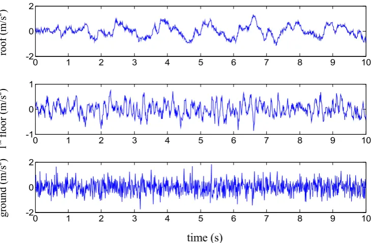
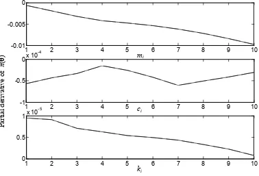
Figure 2.1: The acceleration dataset 1 in ten-story building 43 Figure 2.2: The acceleration dataset 2 in ten-story building 43 Figure 2.3: Gradient using two different methods: reverse algorithmic

differentiation and central finite difference for mass parameters (top figure), damping parameters (middle figure) and stiffness

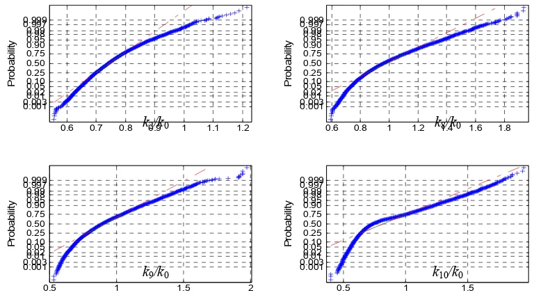
parameters (bottom figure); the curves are indistinguishable 45 Figure 2.4: Pairwise posterior sample plots for some stiffness parameters 50 Figure 2.5: Gaussian probability paper plots for some ki 50

Figure 2.6: Gaussian probability paper plots for some lnki 51

Figure 2.7: The exact (solid) and mean predicted (dashed) time histories of the total acceleration (m/s2) at some unobserved floors together with time histories of the total acceleration that are twice the standard deviation of the predicted robust response from the

mean robust response (dotted) [Dataset 2] 51

Figure 2.8: The exact (solid) and mean (dashed) time histories of the displacement (m) at some unobserved floors together with time histories of the displacement that are twice the standard deviation of the predicted robust response from the mean robust

response (dotted) [Dataset 2] 52

(14)

deviation of the predicted robust response from the mean robust

response (dotted) [Dataset 2] 52

Figure 3.1: Roof acceleration y and base acceleration ab from a linear shear

building with nonclassical damping 93

Figure 3.2: Magnitude of the FFT estimated from the measured roof acceleration data (solid curve) and mean of magnitude of the FFT from the roof acceleration estimated using posterior

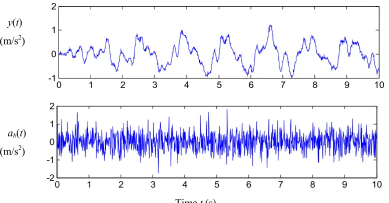
samples from the most probable model class M5 (dashed curve) 93 Figure 3.3: Floor accelerations and base acceleration from a nonlinear

four-story building response (yi(t): total acceleration at the i-th floor;

ab(t): total acceleration at the base) 100

Figure 3.4: The hysteretic restoring force model 100

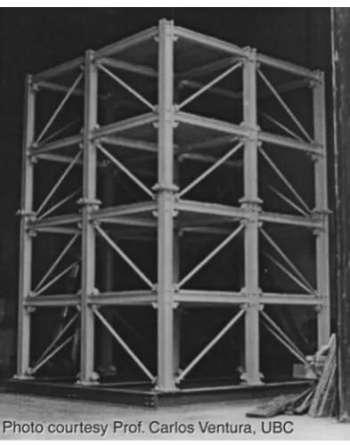
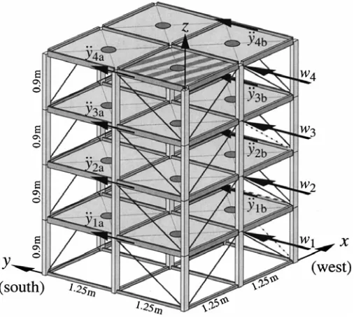
Figure 4.1: IASC-ASCE Structural Health Monitoring Task Group

benchmark structure 124

Figure 4.2: Schematic diagram showing the directions of system output

measurements and input excitations 125

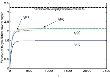
Figure 4.3: The variance of the prediction error for system output in the output equation against time instant (n) given θ=posterior mean

of θ 131

Figure 4.4: The correlation coefficient between prediction errors for different pair of system outputs in the output equation against

time instant (n) given θ=posterior mean of θ for M1 132 Figure 4.5: Posterior robust failure probability against the threshold of

maximum interstory displacements of all floors for M1 (solid

curve) and M2 (dashed curve) 134

Figure 4.6: Posterior (solid curve) robust (for M1) and nominal (dashed) failure probability against the threshold of maximum interstory

(15)

Figure 4.7: Prior robust failure probability against the threshold of

maximum interstory displacements of all floors for M1 136 Figure 4.8: Posterior (solid curve) and prior (dashed) robust (for M2) and

nominal (dot-dashed) failure probability against the threshold of

maximum interstory displacements of all floors 136 Figure 4.9: Posterior robust failure probability against the threshold of

maximum absolute accelerations of all floors for M1 (solid

curve) and M2 (dashed curve) 137

Figure 5.1: Schematic plot for an illustrative example of hierarchical model

classes 146 Figure 5.2: Pairwise sample plots of posterior samples for p(θ| D1(3), M2(1))

normalized by posterior mean 163

Figure 5.3: Pairwise sample plots of posterior samples for p(θ|D1(3), M3(1))

Figure 5.4: Pairwise sample plots of posterior samples for p(θ|D1(3), M4(1))

Figure 5.5: Histogram for posterior samples for p(r|D1(3), M4(3)) 164 Figure 5.6: The failure probability (sorted in increasing order) conditioned

on each posterior sample θ(k) for model class Mj(1), i.e.

P(F|θ(k),D1(3), Mj(1)), for j=2,3,4 165

Figure 5.7: CDF of failure probability P(F|θ, D1(3), Mj(1)), j=2,3,4, estimated

using posterior samples for model class Mj(1) 165

Figure 5.8: CDF of predicted vertical displacement wp at point P in the

target frame structure conditioned on each sample from p(θ|

D1(3), M4(1)) 166

Figure 5.9: Robust posterior CDF of predicted vertical displacement wp at

point P in the target frame structure calculated using the

(16)

Figure 6.1: Schematic plot of importance sampling density 193 Figure 6.1: Posterior robust (solid curve), prior robust (dashed) and

nominal (dot-dashed) failure probabilities plotted against the

threshold of maximum interstory drift of all floors 206 Figure 6.2: Posterior robust (solid curve), prior robust (dashed) and nominal

(dot-dashed) failure probabilities plotted against the threshold

of maximum displacements of all floors relative to the ground 207 Figure 6.3: Posterior robust (solid curve), prior robust (dashed) and nominal

(dot-dashed) failure probability against the threshold of

maximum absolute acceleration of all floors 208 Figure 7.1: South frame elevation (Ching et al. 2006c) 225 Figure 7.2: Hotel column plan (Ching et al. 2006c) 226 Figure 7.3: Exceedance probability for maximum interstory drift 229 Figure 7.4: Predicted time history of interstory displacement of the first

(17)

List of Tables

Table 2.1 Some Basic operations of structural analysis program and the corresponding forward differentiation (FD) and reverse

differentiation (RD) operations 32

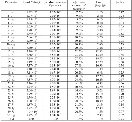
Table 2.2 Statistical results for structural parameter estimates for 10%

noise-to-signal ratio [Dataset 1] 48

Table 2.3 Statistical results for structural parameter estimates for 100%

noise-to-signal ratio [Dataset 2] 49

Table 2.4 The exact natural frequency and damping ratio for each complex

mode [Dataset 2] 53

Table 3.1 Results obtained for Example 1 using the proposed method with

θmax and Q=1 in Equation (3.49) 98

Table 3.2 Posterior means for the natural frequencies, modal damping ratios and roof participation factors for the most probable model class

M5 in Example 1 (exact values in bold) 98

Table 3.3 Results obtained for Example 2 using the proposed method with

θmax and Q=1 in Equation (3.49) 107 Table 4.1 Posterior means and c.o.v. for the uncertain parameters 129

Table 4.2 Results for model class comparison 138

Table 5.1 Number of samples for different cases 151

Table 5.2 Statistical results using data D1(3) from the calibration experiment 158 Table 5.3 Results of predicting δLv using data D1(3)from the calibration

(18)

Table 5.4 Statistical results using data D2(3) from the validation experiment

in addition to D1(3) 172

Table 5.5 Consistency assessment of model classes in predicting δLv using

data D2(3) from the validation experiment in addition to D1(3)

from the calibration experiment 172

Table 5.6 Results of predicting wa using data D2(3) from the validation

experiment in addition to D1(3) from the calibration experiment 175 Table 5.7 Statistical results using data D3(3) from the accreditation

experiment in addition to D1(3) and D2(3) 177 Table 5.8 Consistency assessment of model classes in predicting wa using

data D3(3) from the accreditation experiment in addition to D1(3) from the calibration experiment and D2(3) from the validation

(19)

1

CHAPTER 1

Introduction

(20)

2

quantities related to the environment) should be measured to update models for the system so that a more robust evaluation of the system performance can be obtained.

There are several characteristics of complex dynamic systems making the corresponding stochastic analysis, model and reliability updating computationally very challenging: (1). the system outputs or performance measures cannot be analytically expressed in terms of the uncertain modeling parameters (e.g., when dynamic systems are nonlinear); and (2). the number of uncertain modeling parameters can be quite large; for example, a large number of uncertain parameters are typical in modeling structures which have a large number of degrees of freedom subjected to dynamic excitations such as uncertain future earthquakes (requiring uncertain parameters of the order of hundreds or thousands to specify their discretized ground-motion time histories).

Another problem of much recent interest is model validation for a system which has attracted the attention of many researchers (e.g. Babuška and Oden, 2004; Oberkampf et al. 2004; Babuška et al. 2006; Chleboun 2008; Babuška et al. 2008; Grigoriu and Field 2008; Pradlwarter and Schuëller 2008; Rebba and Cafeo 2008) from many different fields of engineering and applied science because of the desire to provide a measure of confidence in the predictions of system models. In particular, in May 2006, the Sandia Model Validation Challenge Workshop brought together a group of researchers to present various approaches to model validation (Hills et al. 2008). The participants could choose to work on any of three problems; one in heat transfer (Dowding et al. 2008), one in structural dynamics (Red-Horse and Paez 2008) and one in structural statics (Babuška et al. 2008). The difficult issue of how to validate models is, however, still not settled; indeed, it is clear that a model that has given good predictions in tests so far might perform poorly under different circumstances, such as an excitation with different characteristics.

(21)

3

probability axioms. A probability logic approach is used (Beck and Cheung 2009) that is consistent with the Bayesian point of view that probability represents a degree of belief in a proposition but it puts more emphasis on its connection with missing information and information-theoretic ideas stemming from Shannon (1948).

1.1 Stochastic analysis, model and reliability updating of complex systems

Model updating using measured system response, with or without measured excitation, has a wide range of applications in response prediction, reliability and risk assessment, and control of dynamic systems and structural health monitoring (e.g., Vanik et al. 2001; Beck et al. 2001; Papadimitriou et al. 2001; Beck and Au 2002; Katafygiotis et al. 2003; Lam et al. 2004; Yuen and Lam 2006; Ching et al. 2006). There always exist modeling errors and uncertainties associated with the process of constructing a mathematical model of a system and its future excitation, whether it is based on physics or on a black-box ‘nonparametric’ model. Being able to quantify the uncertainties accurately and appropriately is essential for a robust prediction of future response and reliability of structures (Beck and Katafygiotis 1991, 1998; Papadimitriou et al. 2001; Beck and Au 2002; Cheung and Beck 2007a, 2008a, 2008b). Here in this thesis, a fully probabilistic Bayesian model updating approach is adopted, which provides a robust and rigorous framework due to its ability to characterize modeling uncertainties associated with the system and to its exclusive foundation on the probability axioms.

1.1.1 Stochastic system model classes

(22)

4

prior, over this set that quantifies the initial relative plausibility of each predictive model. For simpler presentation, we will usually abbreviate the term “stochastic system model class” to “model class”. Based on M, one can use data D to compute the updated relative plausibility of each predictive model in the set defined by M. This is quantified by the posterior PDF p(θ|D,M) for the uncertain model parameters θ_{ }_D_{which specify a} particular model within M. By Bayes' theorem, this posterior PDF is given by:

1

( | , )θ D M   ( | , ) ( | )D θ M θ M

p c p p (1.1)

where c = p(D|M) = ∫p(D|θ,M)p(θ|M)dθ is the normalizing constant which makes the probability volume under the posterior PDF equal to unity; p(D|θ,M) is the likelihood function which expresses the probability of getting data D based on the predictive PDF for the response given by model θwithin M; and p(θ|M) is the prior PDF for M which one can freely choose to quantify the initial plausibility of each model defined by the value of the parameters θ. For example, through the use of prior information that is not readily built into the predictive PDF that produces the likelihood function, the prior can be chosen to provide regularization of ill-conditioned inverse problems (Bishop 2006). As emphasized by Jaynes (2003), probability models represent a quantification of the state of knowledge about real phenomena conditional on the available information and should not be imagined to be a property inherent in these phenomena, as often believed by those who ascribe to the common interpretation that probability is the relative frequency of “inherently random” events in the “long run”.

(23)

1.1.2 Stochastic system model class comparison

In many engineering applications, we are often faced with the problem of model class selection, that is, based on system data, choosing the most plausible model class from a set of competing candidate model classes to represent the behavior of the system of interest. A model class is a set of parameterized probability models for predicting the behavior of interest together with a prior probability model over this set indicating the relative plausibility of each predictive probability model. The main goal is to handle the tradeoff between the data-fit of a model and the simplicity of the model so as to avoid “overfitting” or “underfitting” the data. Bayesian methods of model selection and hypothesis testing have the advantage that they only use the axioms of probability. In contrast, analysis of multiple models or hypotheses is very difficult in a non-Bayesian framework without introducing ad-hoc measures (Berger and Pericchi 1996). The common selection criteria using p-values (significance tests) are difficult to interpret and can often be highly misleading (Jeffreys 1939, 1961; Lindley 1957, 1980; Berger and Delampady 1987). A common principle enunciated is that, if data is explained equally well by two models, then the simpler model should be preferred (often referred to as Ockham's razor) (Jeffreys 1961). Bayesian methods perform this automatically and systematically (Gull 1988; Mackay 1992; Beck and Yuen 2004) while non-Bayesian methods require introduction of ad-hoc measures to penalize model complexity to prevent overfitting.

(24)

BIC was derived by Schwarz (1978) using Bayesian updating and an asymptotic approach assuming a sufficiently large sample size and that the candidate models all have unique maximum likelihood estimates. Deviance information criterion (DIC) (Spiegelhalter et al. 2002) is a generalization of AIC and BIC. DIC has an advantage that it can be readily calculated from the posterior samples generated by MCMC (Markov chain Monte Carlo) simulation. BIC and DIC are asymptotic approximations to full Bayesian updating at the model class level as the sample size becomes large and they may be misleading when two model classes give similar fits to the data. It was shown empirically by Kass and Raftery (1993) that BIC biases towards simpler models and AIC towards more complicated models as compared with a full Bayesian updating at the model class level, discussed next. The potential of BIC to produce misleading results was pointed out, for example, in Muto and Beck (2008).

Model class comparison is a rigorous Bayesian updating procedure that judges the plausibility of different candidate model classes, based on their posterior probability (that is, their probability conditional on the data from the system). Its application to system identification of dynamic systems that are globally identifiable or unidentifiable was studied in Beck and Yuen (2004) and Muto and Beck (2008), respectively. In these publications, a model class is referred to as a Bayesian model class.

Given a set of candidate model classes M={Mj: j=1,2,…NM}, we calculate the posterior

probability (PM |D_j ,M) of each model class based on system data D by using Bayes’ Theorem:

( ) ( | )

( , )

( | )

j j

j

p P M

P M

p M

 D|M M

M |D

D (1.2)

where P(Mj |M) is the prior probability of each Mj and can be taken to be 1/NM if one

(25)

probability of getting the data D based on Mj and is called the evidence (or sometimes

marginal likelihood) for Mj provided by the data D and it is given by the Theorem of Total

Probability:

( _j) ( _j) ( | _j)

p D|M 



p D| ,Mθ p θ M dθ (1.3)

Although θ corresponds to different sets of parameters and can be of different dimension for different Mj, for simpler presentation a subscript j on θ is not used since explicit

conditioning on Mj indicates which parameter vector θ is involved.

Notice that (1.3) can be interpreted as follows: the evidence gives the probability of the data according to Mj (if (1.3) is multiplied by an elemental volume in the data space) and it

is equal to a weighted average of the probability of the data according to each model specified by Mj, where the weights are given by the prior probability p(θ|Mj)dθ of the

parameter values corresponding to each model. The evidence therefore corresponds to a type of integrated global sensitivity analysis where the prediction p(D|θ,Mj) of each model

specified by θ is considered but it is weighted by the relative plausibility of the corresponding model.

The computation of the multi-dimensional evidence integral in (1.3) is highly nontrivial. The problem involving complex dynamic systems with high-dimensional uncertainties makes this computationally even more challenging. This will be discussed in more detail in a later chapter.

It is worth noting that from (1.3), the log evidence can be expressed as the difference of two terms (Ching et al. 2005; Muto and Beck 2008):

( | , )

ln[ ( | )] [ln( ( | , )] [ln ]

( | ) j

j j

j p

p E p E

p

 θ  θ

θ D M

D M D M

(26)

where the expectation is with respect to the posterior p(θ|D, Mj). The first term is the

posterior mean of the log likelihood function, which gives a measure of the goodness of the fit of the model class Mj to the data, and the second term is the Kullback-Leibler divergence,

or relative entropy (Cover and Thomas 2006), which is a measure of the information gain about Mj from the data D and is always non-negative.

Comparing the posterior probability of each model class provides a quantitative Principle of Model Parsimony or Ockham’s razor (Gull 1989; Mackay 1992), which have long been advocated qualitatively, that is, simpler models that are reasonably consistent with the data should be preferred over more complex models that only lead to slightly improved data fit. The importance of (1.3) is that it shows rigorously, without introducing ad-hoc concepts, that the log evidence for Mj, which controls the posterior probability of this model class

according to (1.2), explicitly builds in a trade-off between the data-fit of the model class and its “complexity” (how much information it takes from the data).

The evidence, and so Bayesian model class selection, may be sensitive to the choice of priors p(θ|Mj) for the uncertain model parameters (Berger and Pericchi 1996). The effect of

(27)

1.1.3 Robust predictive analysis and failure probability updating using

stochastic system model classes

One of the most useful applications of Bayesian model updating is to make robust predictions about future events based on past observations. Let D denote data from available measurements on a system. Based on a candidate model class Mj, all the

probabilistic information for the prediction of a vector of future responses X is contained in the posterior robust predictive PDF for Mj given by the Theorem of Total Probability

(Papadimitriou et al. 2001):

( | _j) ( | , , _j) ( | _j)

p X D,M 



p X θ D M p θ D,M dθ (1.5)

The interpretation of (1.5) is similar to that given for (1.3) except now the prediction p(X|θ,D,Mj) of each model specified by θ is weighted by its posterior probability

p(θ|D, Mj)dθbecause of the conditioning on the data D. If this conditioning on D in (1.5) is

dropped so, for example, the prior p(θ|Mj) is used in place of the posterior p(θ|D, Mj), the

result p(X|Mj) of the integration is the prior robust predictive PDF.

Many system performance measures can be expressed as the expectation of some function

g(X) with respect to the posterior robust predictive PDF in (1.5) as follows:

[ ( ) |E g X D,M_j]



g X( ) ( | ,p X D M_j)dX (1.6)

Some examples of important special cases are:

1) g(X)=IF(X), which is equal to 1 if XF and 0 otherwise, where F is a region in the

(28)

2) g(X)=X, then the integral in (1.6) becomes the robust mean response;

3) g(X)=(X-E[X|D, Mj])(X-E[X|D, Mj])T, then the integral in (1.6) is equal to the robust

covariance matrix of X.

The Bayesian approach to robust predictive analysis requires the evaluation of multi-dimensional integrals, such as in (1.5), and this usually cannot be done analytically. For problems involving complex dynamic systems with high-dimensional uncertainties, this can be computationally challenging. This will be discussed in more detail in a later chapter.

If a set of candidate model classes M={Mj: j=1,2,…NM} is being considered for a system,

all the probabilistic information for the prediction of future responses X is contained in the hyper-robust predictive PDF for M given by the Theorem of Total Probability (Muto and Beck 2008):

1

( | ) M ( | , ) ( | , )

N

j j

j

p M p P M





X D, X D M M D (1.7)

where the robust predictive PDF for each model class Mj is weighted by its posterior

probability P(Mj|D, M) from (1.2). Equation (1.7) is also called posterior model averaging

in the Bayesian statistics literature (Raftery et al. 1997, Hoeting et al. 1999).

Let F denote the events or conditions leading to system failure (unsatisfactory system performance). The hyper-robust failure probability P(F|D,M) based on M is then given by (Cheung and Beck 2008g, 2009a, 2009b):

1

( | ) M ( | , ) ( | , )

N

j j

j

P F M P F P M





D, D M M D (1.8)

(29)

1.2 Outline of the Thesis

In this thesis, the focus is on stochastic system analysis, model and reliability updating of complex systems, with special attention to complex dynamic systems which can have high-dimensional uncertainties, which are very challenging. New methods are developed to solve these problems. Most of the methods developed in this thesis are intended to be very general without requiring special assumptions regarding the system. A new methodology is also developed to tackle the challenging model validation problem. Novel methods for updating robust failure probability are also developed.

In Chapter 2, model updating problems for complex systems which have high-dimensional parameter uncertainties within a stochastic system model class are considered. To solve the challenging computational problems, stochastic simulation methods, which are reliable and robust to problem complexity, are proposed. Markov Chain Monte Carlo simulation methods are presented and reviewed. An advanced Markov Chain Monte Carlo simulation method namely Hybrid Monte Carlo simulation method is investigated. Practical issues for the feasibility of this method to solve Bayesian model updating problems of complex dynamic systems involving high-dimensional uncertainties are addressed. Improvements are proposed to make it more effective and efficient for solving such model updating problems. New formulae for Markov Chain convergence assessment are derived. The effectiveness of the proposed approach is illustrated with an example for Bayesian model updating of a structural dynamic model with many uncertain parameters. New stochastic simulation algorithms created by combining state-of-the-art stochastic simulation algorithms are also presented.

(30)

system. Another problem of interest is to tackle cases where more than one model class has significant posterior probability and each of these give different predictions. Bayesian model class averaging then provides a coherent mechanism to incorporate all the considered model classes in the probabilistic predictions for the system. However, both Bayesian model class selection and averaging require calculation of the evidence of the model class based on the system data, which requires the computation of a multi-dimensional integral involving the product of the likelihood and prior defined by the model class. Methods for solving the computationally challenging problem of evidence calculation are reviewed and new methods using posterior samples are presented.

(31)

In Chapter 5, the problem of model validation of a system is considered. Here, we consider the problem where a series of experiments are conducted that involve collecting data from successively more complex subsystems and these data are to be used to predict the response of a related more complex system. A novel methodology based on Bayesian updating of hierarchical stochastic system model classes using such experimental data is proposed for uncertainty quantification and propagation, model validation, and robust prediction of the response of the target system. The proposed methodology is applied to the 2006 Sandia static-frame validation challenge problem to illustrate our approach for model validation and robust prediction of the system response. Recently-developed stochastic simulation methods are used to solve the computational problems involved.

In Chapter 6, a newly-developed approach based on stochastic simulation methods is presented, to update the robust reliability of a dynamic system. The efficiency of the proposed approach is illustrated by a numerical example involving a hysteretic model of a building.

(32)

CHAPTER 2

Bayesian updating of stochastic system model classes

with a large number of uncertain parameters

(33)

accuracy in approximating this probability distribution in other regions of the uncertain parameter space. It may therefore lead to a poor estimate of robust failure probability. Other analytical approximations to the posterior PDF such as the variational approximation (Beal 2003) suffer similar problems as Laplace’s method of asymptotic approximation.

Thus, in recent years, focus has shifted from analytical approximations to using stochastic simulation methods in which samples consistent with the posterior PDF p(θ|D,M) are generated. In these methods, all the probabilistic information encapsulated in p(θ|D,M) is characterized by posterior samples _θ( )k _{, k=1,2,...,K:}

( ) 1

1

( | ) ( )

K

k k

p

K  







θ D,M θ θ (2.1)

With these samples, the integral in (1.5) can be approximated by:

( ) 1

1

( | ) K ( | k , , )

k

p p

K 





X D,M X θ D M (2.2)

Samples of X can then be generated from each of the _p_{( |}_X _θ( )k _{, , )}

D M with equal probability. The probabilistic information encapsulated inp( |X D,M)is characterized by these samples of X.

(34)

Ching et al. 2006, Ching and Cheng 2007, Muto and Beck 2008) were proposed to solve the Bayesian model updating problem more efficiently.

Probably the most well-known MCMC method is the Metropolis-Hastings (MH) algorithm (Metropolis et al. 1953, Hastings 1970) which creates samples from a Markov Chain whose stationary state is a specified target PDF. In principle, this algorithm can be used to generate samples from the posterior PDF but, in practice, its direct use is highly inefficient because the high probability content is often concentrated in a very small volume of the parameter space. Beck and Au (2000, 2002) proposed an approach which combines the idea from simulated annealing with the MH algorithm to simulate from a sequence of target PDFs, where each such PDF is the posterior PDF based on an increasing amount of data. The sequence starts with the spread-out prior PDF and ends with the much more concentrated posterior PDF. The samples from a target PDF in the sequence are used to construct a kernel sampling density which acts as a global proposal PDF for the MH procedure for the next target PDF in the sequence. The success of this approach relies on the ability of the proposal PDF to simulate samples efficiently for each intermediate PDF. However, in practice, this approach is only applicable in lower dimensions since in higher dimensions, a prohibitively large number of samples are required to construct a good global proposal PDF which can generate samples with reasonably high acceptance probability. In other words, if the sample size for the particular level is not large enough, most of the candidate samples generated by the proposal PDF will be rejected by the MH algorithm, leading to many repeated samples, slowing down greatly the exploration of the high probability region of the posterior PDF.

(35)

intermediate PDFs such that the last PDF in the sequence is p(θ|D,M). The main difference is in the way samples are simulated: TMCMC uses re-weighting and re-sampling techniques on the samples from a target PDF πi(θ) in the sequence to generate initial

samples for the next target PDF πi+1(θ) in the sequence. A Markov chain of samples is initiated from each of these initial samples using the MH algorithm with stationary distribution πi+1(θ): each sample is generated from a local random walk using a Gaussian

proposal PDF centered at the current sample of the chain that has a covariance matrix estimated by importance sampling using samples from πi(θ). TMCMC has several

advantages over the previous approaches: 1) it is more efficient; 2) it allows the estimation of the normalizing constant c of p(θ|D,M), which is important for Bayesian model class selection (Beck and Yuen 2004). However, TMCMC has potential problems in higher dimensions, which need further attention: 1) the initial samples from weighting and re-sampling of samples in πi(θ), in general, do not exactly follow πi+1(θ), so the Markov

chains must “burn-in” before samples follow πi+1(θ), requiring a large amount of samples to

be generated for each intermediate level; 2) in higher dimensions, convergence to πi+1(θ)

can be very slow when using the MH algorithm based on local random walks, as in TMCMC.This adverse effect becomes more pronounced as the dimension increases and it introduces more inaccuracy into the statistical estimates based on the samples.

(36)

parameters is illustrated with a simulate data example involving a 10-story building. Hybrid algorithms based on Markov Chain Monte Carlo simulation algorithms are presented at the end of the chapter. Part of the materials presented in this chapter are presented in Cheung and Beck (2007c;2008a).

2.1 Basic Markov Chain Monte Carlo simulation algorithms

2.1.1 Metropolis-Hastings algorithm and its features

The complete Metropolis-Hastings Algorithm for simulating samples from a target distribution π(θ) (where π(θ) need not be normalized) can be summarized as follows:

1. Initialize θ(0) by choosing it deterministically or randomly (see discussion in Section 4.3);

2. Repeat step 3 below for i = 1,…, N.

3. In iteration i, let the most recent sample be θ(i-1), then do the following to simulate a new sample θ(i).

i.) Randomly draw a candidate sample θc from some proposal distribution

q(θc |θ(i-1));

ii.) Accept θ(i) = θc with probability Pacc given as follows:

( 1)

( 1) ( 1)

( ) ( | )

min{1, }

( ) ( | )

i

c c

acc i i

c q P

q

 



 

 θ θ θ

θ θ θ (2.3)

If rejected, then θ(i)_{= θ}(i-1)_{, i.e. the (i-1)}th_{sample is repeated.}

The proposal PDF q(θc |θ(i)) should be of a form that allows an easy and direct drawing of

θc given θ(i). The choice of θ(0) and q(θc |θ(i)) affects the convergence rate of the algorithm.

(37)

The most common choice of q(θc|θ(i)) is a symmetric proposal PDF in which

q(θc|θ(i)) = q(θ(i)|θc); for example, the local random walk Gaussian proposal PDF is popular,

which is centered at the current sample θ(i) with some predetermined covariance matrix C. This proposal PDF allows a local exploration of the neighborhood of the current sample. Its main drawback is that in higher dimensions, it becomes infeasible to construct a proposal PDF which can explore the region of high probability content efficiently and effectively while at the same time maintaining a reasonable acceptance probability of the candidate sample. Another possible choice is the non-adaptive proposal PDF in which the simulation of the candidate sample is independent of the current sample, i.e., q(θc|θ(i)) = q(θc). For this

type of proposal PDF to work, it has to be very similar to the target PDF. However, in general, the construction of such PDFs is infeasible in higher dimensions, even when some samples of the target PDF are available.

2.1.2 Gibbs Sampling algorithm and its features

Consider θas a composition of n vector components which do not need to be of the same dimension, i.e., θ = [θ1,θ2,…,θn], such that the conditional probability distribution π(θj|{θ -j}) of θi given all the other components is known. The complete algorithm of Gibbs

sampling for simulating samples of a target distribution π(θ) (where π(θ) need not be normalized) can be summarized as follows:

1. Initialize θ(0) either deterministically or randomly; 2. Repeat step 3 below for i = 1,…, N.

3. In iteration i, let the most recent sample be θ(i-1) = [ ( 1) 1

i

θ , ( 1) 2

i

θ ,…, ( 1)i n



θ ], then do the following to simulate a new sample θ(i)= [ ( )

1

i θ , ( )

2

i

θ ,…, ( )i n

θ ]: for each j=1,2,…, n, randomly draw ( )i

j

θ from π( ( )i j θ | ( )

1

i

θ ,…, ( ) 1

i j

θ , ( 1) 1

i j

 

θ ,…, ( 1)i n



θ }.

(38)

case of the Metropolis-Hastings algorithm where the acceptance probability is 1 if

π( ( )i j θ | ( )

1

i

θ ,…, ( ) 1

i j

θ , ( 1) 1

i j

 

θ ,…, ( 1)i n



θ } is in a form which allows direct and easy drawing of

( )i j

θ ; if this is not the case, one can use, for example, the Metropolis-Hastings algorithm: draw a candidate c

j

θ from some chosen proposal q( c j θ | ( )

1

i

θ ,…, ( ) 1

i j

θ , ( 1)i j



θ , ( 1) 1

i j

 

θ ,…, ( 1)i n



θ ) which allows easy and direct random drawing, and accept ( )i

j θ = c

j

θ with probability Pacc

where:

( ) ( ) ( 1) ( 1)

1 1 1

( 1) ( ) ( ) ( 1) ( 1)

1 1 1

( ) ( ) ( 1) ( 1) ( 1)

1 1 1

( 1) ( ) ( ) ( 1

1 1 1

( | ,..., , ,..., ) ( | ,..., , ,..., ) min{1,

( | ,..., , , ,..., ) ( | ,..., , ,

c i i i i

j j j n

i i i i i

j j j n

acc c i i i i i

j j j j n

i i i c i

j j j

P q q                     

θ θ θ θ θ

θ θ θ θ θ

θ θ θ θ θ θ

θ θ θ θ θ ) ( 1)

} ,..., i )

n



θ

(2.4)

If rejected, then ( )i j

θ = ( 1)i j



θ . It should be noted that the convergence of the Gibbs sampling algorithm can be slowed down if there is a strong correlation between components.

2.2 Hybrid Monte Carlo Method

Hybrid Monte Carlo Method (HMCM) was first introduced by Duane et al. (1987) as a MCMC technique for sampling from complex distributions by combining Gibbs sampling, MH algorithm acceptance rule and deterministic dynamical methods. By avoiding the local random walk behavior exhibited by the MH algorithm through the use of dynamical methods, HMCM can be much more efficient. The advantage of HMCM is even more pronounced when sampling the highly-correlated parameters from posterior distributions that are often encountered in Bayesian structural model updating. However, the potential of HMCM has not yet been explored in Bayesian structural model updating.

(39)

(Hamiltonian function) of the fictitious dynamical system is defined by:H( , ) = ( ) + θp V θ W( )p , where its potential energy V(θ) = −lnπ(θ) and its kinetic energy W(p) depends only on p and some chosen positive definite ‘mass’ matrix

D D



M  :

T 1

( ) / 2

W _p __{p M p} _(2.5)

Since M can be chosen at our convenience, it is taken as a diagonal matrix with entries Mi,

i.e., M = diag(Mi). A joint distribution f(θ, p) over the phase space (θ, p) is considered:

( , ) exp( ( , ))

f θ p K H θ p (2.6)

where K is the normalizing constant. Clearly,

T 1

( , ) ( ) exp( / 2)

f _θ_p _K _θ _{p M p}_  _(2.7)

Note that π(θ) can be unnormalized (the usual situation that arises when constructing a posterior PDF) since its normalizing constant can be absorbed into K. Samples of θ from

π(θ) can be obtained if we can sample (θ, p) from the joint distribution f(θ, p) in (2.7). Note that (2.7) shows that p andθ are independent and the marginal distributions of θand p are respectively π(θ) and N(0, M), a Gaussian distribution with zero mean and covariance matrix M.

Using Hamilton’s equations, the evolution of (θ, p) through fictitious time t is given by:

( )

d H

V dt



    

p

θ

θ (2.8)

1

d H

dt





 



θ

M p

p (2.9)

(40)

1. The total energy H remains constant throughout the evolution;

2. The dynamics are time reversible, i.e., if a trajectory initiates at (θ’, p’) at time 0 and ends at (θ’’, p’’) at time t, then a trajectory starting at (θ’’, p’’) at time 0 will end at (θ’, p’) at time –t (or, equivalently, a trajectory starting at (θ’’, -p’’) at time 0 will end at (θ’, -p’) at time t).

3. The volume of a region of phase space remains constant (by Liouville’s theorem). 4. The above evolution of (θ, p) leaves f(θ, p) in (2.7) as the stationary distribution

(Duane et al. 1987); in particular, if θ(0) follows the distribution π(θ), then after time t, θ(t) also follows π(θ). Duane et al. (1987) proved this by showing the detailed balance condition for the stationarity of a Markov Chain is satisfied. In Appendix 2A, we provide an alternative proof to show that f(θ, p) is actually the stationary distribution using the diffusionless Fokker-Planck equation.

If we start with θ(0) and draw a sample p(0) from N(0, M), then solve the Hamiltonian dynamics (2.8) and (2.9) for some time t, the final values (θ(t), p(t)) will provide an independent sample θ(t) from π(θ). In practice, (2.8) and (2.9) have to be solved numerically using some time-stepping algorithm such as the commonly-used leapfrog algorithm (Duane et al. 1987). In this latter case, for time step δt, we have:

( ) ( ) ( ( ))

2 2

t t

t  t  V t

p p θ (2.10)

1

( ) ( ) ( )

2 t tt  t t  t

θ θ M p (2.11)

( ) ( ) ( ( ))

2 2

t t

tt  t  V tt

p p θ (2.12)

Equations (2.10)-(2.12) can be reduced to:

1

( ) ( ) [ ( ) ( ( ))]

2 t

tt  t t  t  V t

(41)

( ) ( ) [ ( ( )) ( ( ))] 2

t

tt  t  V t  V tt

p p θ θ (2.14)

The gradient of V with respect to θ needs to be calculated once only for each time instant since its value in the last step in the above algorithm at time t is the same as the first step at time t+δt.

2.2.1 HMCM algorithm

The complete algorithm of HMCM can be summarized as follows (for some chosen M, δt and L):

1. Initialize θ0 (discussion of the choice of this is presented in a later section) and simulate p0 such that p0~N(0,M);

2. Repeat step 3 below for i = 1,…, N.

3. In iteration i, let the most recent sample be (θi-1, pi-1), then do the following to

simulate a new sample (θi, pi):

i) Randomly draw a new momentum vector p’ from N(0, M);

ii) Initiate the leapfrog algorithm with (θ(0), p(0)) =(θi-1, p’) and run the algorithm for L time steps to obtain a new candidate sample (θ”, p”) = (θ(t+Lδt), p(t+Lδt))

iii) Accept (θi, pi)= (θ”, p”) with probability Pacc = min{1,exp(ΔH)} where

ΔH =H(θ”, p”)H(θi-1, p’). If rejected, then (θi, pi)= (θi-1, p’), so V(θi)=

V(θi-1) and V( )θi  V(θi1).

2.2.2 Discussion of algorithm

(42)

( (θ n t ), (p n t ))h( ((θ n1) ), ((t p n1) ))t (2.15)

where h corresponds to the mapping produced by the time-stepping algorithm, e.g., leap frog. The candidate sample (θc, pc) is then the output of the following:

1/2

( , )_c _c ( (... ( (0), (0))) ( (... ( (0), ))

L L

 

θ p h h h___ θ p h h h___ θ M z (2.16)

where z is a standard Gaussian vector with independent components N(0,1). Thus Steps 2(i) and (ii) together can be viewed as drawing a candidate sample from a global transition PDF which is non-Gaussian if the mapping h is nonlinear (the usual case). Applying mapping h

multiple times leads to the exploration of the phase space further away from the current point, towards the higher probability region, avoiding the local random walk behavior of most MCMC methods. Therefore, HMCM can be viewed as a combination of Gibbs sampling (Step 2(i)) followed by a Metropolis algorithm step (Step 2(iii)) in an enlarged space with an implied complicated proposal PDF that enhances a more global exploration of the phase space than using a simple Gaussian PDF centered at the current sample, as adopted for the proposal PDF in the random walk Metropolis algorithm.

Although the leapfrog algorithm is volume preserving (sympletic) and time reversible, H does not remain exactly constant due to the systematic error introduced by the discretization of (2.8) and (2.9) with the leapfrog algorithm. To keep f(θ, p) as the invariant PDF of the Markov chain, and thus keep π(θ) invariant, this systematic error needs to be corrected through the Metropolis acceptance/rejection step in Step 2(iii). The probability of acceptance, Pacc, in Step 2(iii) depends only on the difference in energy ΔH between H for

the candidate sample (θ”, p”) and H for (θi-1, p’), which initiates the current leapfrog steps.

(43)

It is worth noting that when L=1, HMCM is similar to an algorithm in which the evolution of θfollows the following Itô stochastic differential equation:



1 1/2

1

( ) ( ( )) ( )

2

d tθ   MV θ t dtM dW t (2.17)

where _W( )_t __D_{is a standard Wiener process. The discretized version corresponding to} (2.17) is:

1 1/2

c

1

( ) ( ( ))

2

t  V t t  t

   

θ θ M θ M z (2.18)

where θc is the candidate sample and z is a standard Gaussian vector with independent components that are N(0,1). Thus, it is interesting to see that when L=1, the candidate sample of HMCM is drawn from the Gaussian proposal PDF:

 1 

c /2 c c

1 1

( | ( )) exp( ( ( ( ))) ( ( ( ))))

(2 | |) 2

T D

q t  t  t





   

θ θ θ θ C θ θ

C (2.19)

where the mean ( ( ))θ t and the covariance matrix C are given by the following:

_{( ( ))} _{( )} 1 1 _{ln ( ( ))}

2

t t t t

 _θ __θ _ _M _  _θ _(2.20)

1/2 1/2 1

E[(  __{t t}( ))(  __{t t}( )) ]T __t 

 

C M z M z M (2.21)

(44)

There are 3 parameters, namely M, δt and L, that need to be chosen before performing HMCM. If δt is chosen to be too large, the energy H at the end of the trajectory will deviate too much from the energy at the start of the trajectory which may lead to frequent rejections due to the Metropolis step in Step 2(iii). Thus, δt should be chosen small enough so that the average rejection rate due to the Metropolis step is not too large, but not too small that effective exploration of the high probability region is inhibited; a procedure for optimally choosing δt is presented later. For each dynamic evolution in the deterministic Step 2(ii), L can be randomly chosen from a discrete uniform distribution from 1 to some preselected Lmax to avoid getting into a resonance condition (Mackenzie, 1989) (although it occurs

rarely in practice) in which the trajectories from Step 2(ii) go around the same closed trajectory for a number of cycles. Matrix M can be chosen to be a diagonal matrix diag(M1 ,…, MD) where Mi is 1 for each i if the components of θare of comparable scale.

This can be ensured by initially normalizing the uncertain parameters θ.

2.3 Proposed improvements to Hybrid Monte Carlo Method

2.3.1 Computation of gradient of V(

θ

) in implementation of HMCM

In general,V( )θ  ln ( ) θ cannot be found analytically, so numerical methods must be used to find its value. The most common method uses finite differences. The computation of the gradient vector V( )θ using finite differences requires either D or 2D evaluations of V where D is the dimension of the uncertain parameters.

(45)

for differentiation judiciously to the elementary functions, the building blocks forming the program for output analysis, and to calculate the output and its sensitivity with respect to the input parameters simultaneously in one code. Unlike the classical finite difference methods which have truncation errors, one can obtain the derivatives within the working accuracy of the computer using algorithmic differentiation.

There are two ways in which the differentiation can be performed: forward differentiation or reverse differentiation. In forward differentiation, the differentiation is carried out following the flow of the program for the output analysis and performing the chain rule in the usual forward manner. To illustrate the idea behind the forward code differentiation, consider the following simple example for the program for computing the output function

( )

y=hθ Î :

, 1, 2,..., j j

w =θ j= D

Repeat for j=D+1,…, p

{ }

_{_1,2,..., ₁_}

( )

j j _{k k} j w =h w _Î

-p y=w

where hj’s can be elementary arithmetic operations or standard scalar functions on modern

computer or mathematical softwares. The computation of the corresponding derivatives is practically free once the function itself has been computed. The corresponding code for computing the sensitivity Sy of y with respect to θis as follows:

, 1, 2,..., j j

w =θ j= D

, 1, 2,..., j j

w j D

(46)

{ }

_{_1,2,..., ₁_}

( )

j

j j k k B j w =h w _{Î Í}

-{1,2,..., 1}

k j

j

j k

k h

w w

w Î

-¶

 = 

¶

å

p y=w

y wp

S = 

where the forward derivative T

1 2

[ / , / ,..., / ]

j j j j D

w w θ w θ w θ

 = ¶ ¶ ¶ ¶ ¶ ¶ is the sensitivity

of w_jwith respect to θ and ej is a D-dimensional unit vector with the j-th component being

1 and all the other components being 0. Assuming the dimension of Bj is Nj and the

calculation of each w_j requires at most KNj arithmetic operations for some fixed constant

K, here we can find the amount of computations required to calculate Sy: KNj+DNj

arithmetic operations are required to calculate each intermediate gradient vectorw_j. The total number of arithmetic operations for the calculation of Sy are

1

( )

p

j j

j D

KN DN

 





and that for the calculation of y are

1

p j j D

KN

 



. Thus the computational

effort required by forward differentiation increases linearly with D. However, as mentioned earlier, forward differentiation does not incur errors as classical finite difference methods do and is accurate to the computer accuracy.

(47)

later showed that Wolfe’s assertion is actually a theorem if the ratio, being on average 1.5, is replaced by an upper bound of 5. Rather than calculating the sensitivity of every intermediate variable with respect to the parameters θ as in forward differentiation, reverse differentiation is a form of algorithmic differentiation which starts with the output variables and computes the sensitivity of the output with respect to each of the intermediate variables. The biggest advantage of reverse differentiation is seen when the output variable is a scalar and the corresponding gradient with respect to high-dimensional input parameters is of interest. Under this circumstance, it has been shown (Griewank 1989) that the computational effort required by reverse differentiation to calculate the gradient accurately is only between 1 to 4 times of that required to calculate the output function, regardless of the dimension of the input parameters. This situation applies to our problem since the output variable of interest is the scalar function V.

To illustrate the idea behind the reverse differentiation, consider the same example as for forward differentiation. The code for computing the sensitivity sy of y with respect to θ

usingreverse differentiation is as follows:

, 1, 2,..., j j

w  j D

0, 1, 2,..., j

w  j D

 

1,2,..., 1

( )

k Bj j

j j k

w h w

   

0 j w 

(48)

1 y

p w y

Repeat for j=p, p-1,…, D+1

, {1, 2,..., 1} j

k k j j

k h

w w w k B j

w



    



  

, 1, 2,..., j w jj D

   

where y w~, , ~ j ~_j denotes the reverse derivatives    y y/ , /y w_j,  y/ _j respectively.

Thus sy = [

~ 1

 , ~₂, …, ~_D]. The total number of arithmetic operations for the calculation of

sy are

1

( )

p

j j j D

KN N

 





and that for the calculation of y are

1

p j j D

KN

 



. Thus the

computational effort required by reverse differentiation is independent of D. It is noted that the approach presented above can be extended to compute higher-order derivatives.

Structural analysis programs usually involve program statements which perform vector and matrix operations and solve implicit linear equations. Higher-dimensional implicit linear equations are involved and the number of elementary intermediate variables required to store information for differentiation is large. Thus, it is more efficient to perform differentiation at the vector or matrix levels.

(49)

differentiation at the vector or matrix levels (Appendix 2B). Those operations for the forward differentiation are very straightforward and obvious and no derivation will be given. Table 2.1 summarizes these operations. ˆY denotes some matrix whose (i,j)-th entry is the forward partial derivative Y /ij k of the (i,j)-th entry of a matrix Y with respect to some _k and Y denote some matrix whose (i,j)-th entry is the reverse partial derivative

/ Y_ij V

  of the output function V with respect to the (i,j)-th entry of Y. In the first column of Table 1, each equation carries out a certain operation inside the program. The left hand side of the equation in each of the row except the last row gives the intermediate output corresponding to the inputs on the right hand side which can in turn be the intermediate output resulting from the previous program statement. The last row shows an implicit equation for solving a certain intermediate output v given U and w. The second column

shows the forward differentiation operations. The derivatives of the intermediate output with respect to some variable _k are computed given the values of the derivatives of the input with respect to the same variable, which are obtained from previous steps in the program. The third column shows the reverse differentiation operations. All the reverse partial derivatives are initialized to be zero at the beginning of the reverse differentiation. The reverse partial derivative of the output function V with respect to the intermediate input is incremented by the amount shown in the table given the values of the derivatives of the output function V with respect to the intermediate output that the input affects. For example, consider the two consecutive operations in the middle of a program:



  

w u v

z u

(50)

 

     

;

; ;

T

  

   

u u z u z

u u w v v w

 

Based on the results developed above, a very efficient reverse differentiation code has been obtained for the case involving linear dynamical systems (Appendix 2B).

The idea of algorithmic differentiation can be extended to treat the case with nonsmooth intrinsic elementary functions (for example, those functions involving absolute signs and those problems involving hysteretic models). The ideas presented above could be incorporated in commercial structural analysis softwares to create a program code for a more accurate and efficient sensitivity analysis accompanying response analysis. The coding needs only one time effort, which can be made automatic by writing a program with the rules for “algorithm differentiation” developed above using object oriented programs such as Fortran, C, C++ or Matlab such that the code for sensitivity analysis can be created automatically given the original program code for response analysis. The idea is to write a command code to read the code for response analysis and then do the “translation” and creation of the differentiation code. It should be noted that the above methods can be easily extended if the sensitivity of a vector function is of interest.