Macroscopic coherent structures in a stochastic neural network: from interface dynamics to coarse grained bifurcation analysis

DOI 10.1007/s00285-016-1070-9

Mathematical Biology

Macroscopic coherent structures in a stochastic neural

network: from interface dynamics to coarse-grained

bifurcation analysis

Daniele Avitable1 · Kyle C. A. Wedgwood2

Received: 13 March 2016 / Revised: 6 October 2016 / Published online: 1 February 2017 © The Author(s) 2017. This article is an open access publication

Abstract We study coarse pattern formation in a cellular automaton modelling a spatially-extended stochastic neural network. The model, originally proposed by Gong and Robinson (Phys Rev E 85(5):055,101(R),2012), is known to support stationary and travelling bumps of localised activity. We pose the model on a ring and study the existence and stability of these patterns in various limits using a combination of ana-lytical and numerical techniques. In a purely deterministic version of the model, posed on a continuum, we construct bumps and travelling waves analytically using standard interface methods from neural field theory. In a stochastic version with Heaviside fir-ing rate, we construct approximate analytical probability mass functions associated with bumps and travelling waves. In the full stochastic model posed on a discrete lat-tice, where a coarse analytic description is unavailable, we compute patterns and their linear stability using equation-free methods. The lifting procedure used in the coarse time-stepper is informed by the analysis in the deterministic and stochastic limits. In all settings, we identify the synaptic profile as a mesoscopic variable, and the width of the corresponding activity set as a macroscopic variable. Stationary and travelling bumps have similar meso- and macroscopic profiles, but different microscopic struc-ture, hence we propose lifting operators which use microscopic motifs to disambiguate them. We provide numerical evidence that waves are supported by a combination of

Kyle Wedgwood was generously supported by the Wellcome Trust Institutional Strategic Support Award (WT105618MA).

B

1 _{Centre for Mathematical Medicine and Biology, School of Mathematical Sciences, University of} Nottingham, Nottingham NG2 7RD, UK

high synaptic gain and long refractory times, while meandering bumps are elicited by short refractory times.

Keywords Multiple scale analysis·Mathematical neuroscience·Refractoriness· Spatio-temporal patterns·Equation-free modelling·Markov chains

Mathematics Subject Classification 37N25·34E13·35B34

1 Introduction

In the past decades, single-neuron recordings have been complemented by multi-neuronal experimental techniques, which have provided quantitative evidence that the cells forming the nervous systems are coupled both structurally (Braitenberg and Schüz 1998) and functionally (for a recent review, seeYuste(2015) and references therein). An important question in neuroscience concerns the relationship between electrical activity at the level of individual neurons and the emerging spatio-temporal coher-ent structures observed experimcoher-entally using local field potcoher-ential recordings (Einevoll et al. 2013), functional magnetic resonance imaging (Heuvel and Hulshoff Pol 2010) and electroencephalography (Nunez and Srinivasan 2006).

There exist a wide variety of models describing activity at the level of an indi-vidual neuron (Izhikevich 2007;Ermentrout and Terman 2010), and major research efforts in theoretical and computational neuroscience are directed towards coupling neurons in large-dimensional neural networks, whose behaviour is studied mainly via direct numerical simulations (Izhikevich and Edelman 2008;Fairhall and Sompolinsky 2014).

A complementary approach, dating back toWilson and Cowan(1972, 1973) and

Amari(1975,1977), foregoes describing activity at the single neuron level by repre-senting averaged activity across populations of neurons. Theseneural field modelsare nonlocal, spatially-extended, excitable pattern-forming systems (Ermentrout 1998) which are often analytically tractable and support several coherent structures such as localised radially-symmetric states (Werner and Richter 2001;Laing et al. 2002;

Laing and Troy 2003; Bressloff and Kilpatrick 2011; Faye et al. 2013), localised patches (Laing and Troy 2003;Rankin et al. 2014;Avitabile and Schmidt 2015), pat-terns on lattices with various symmetries (Ermentrout and Cowan 1979; Bressloff et al. 2001), travelling bumps and fronts (Ermentrout and McLeod 1993; Bressloff 2014), rings (Owen et al. 2007;Coombes et al. 2012), breathers (Folias and Bressloff 2004,2005;Folias and Ermentrout 2012), target patterns (Coombes et al. 2013), spi-ral waves (Laing 2005) and lurching waves (Golomb and Ermentrout 1999;Osan and Ermentrout 2001;Wasylenko et al. 2010) [for comprehensive reviews, we refer the reader toBressloff 2012,2014].

Recent studies have analysed neural fields with additive noise (Hutt et al. 2008;

Bressloff 2009, 2010;Baladron et al. 2012), the development of a rigorous theory of multi-scale brain models is an active area of research.

Numerical studies of networks based on realistic neural biophysical models rely almost entirely on brute-force Monte Carlo simulations (for a very recent, remarkable example, we refer the reader to (Markram et al. 2015)). With thisdirect numerical sim-ulationapproach, the stochastic evolution of each neuron in the network is monitored, resulting in huge computational costs, both in terms of computing time and memory. From this point of view, multi-scale numerical techniques for neural networks present interesting open problems.

When few clusters of neurons with similar properties form in the network, a significant reduction in computational costs can be obtained by population density methods (Omurtag et al. 2000; Haskell et al. 2001), which evolve probability den-sity functions of neural subpopulations, as opposed to single neuron trajectories. This coarse-graining technique is particularly effective when the underlying microscopic neuronal model has a low-dimensional state space (such as the leaky integrate-and-fire model) but its performance degrades for more realistic biophysical models. Develop-ments of the population density method involve analytically derived moment closure approximations (Cai et al. 2004;Ly and Tranchina 2007). Both Monte Carlo simu-lations and population density methods give access only to stable asymptotic states, which may form only after long-transient simulations.

An alternative approach is offered by equation-free (Kevrekidis et al. 2003;

Kevrekidis and Samaey 2009) andheterogeneous multiscalemethods (Weinan and Engquist 2003;Weinan et al. 2007), which implement multiple-scale simulations using an on-the-fly numerical closure approximations. Equation-free methods, in particular, are of interest in computational neuroscience as they accelerate macroscopic simu-lations and allow the computation of unstable macroscopic states. In addition, with equation-free methods, it is possible to perform coarse-grained bifurcation analysis using standard numerical bifurcation techniques for time-steppers (Tuckerman and Barkley 2000).

The equation-free framework (Kevrekidis et al. 2003;Kevrekidis and Samaey 2009) assumes the existence of a closed coarse model in terms of a few macroscopic state variables. The model closure is enforced numerically, rather than analytically, using a coarse time-stepper: a computational procedure which takes advantage of knowledge of the microscopic dynamics to time-step an approximated macroscopic evolution equation. A single coarse time step from timet0to timet1is composed of three stages:

(i)lifting, that is, the creation of microscopic initial conditions that are compatible with the macroscopic states at timet0; (ii)evolution, the use of independent realisations

of the microscopic model over a time interval [t0,t1]; (iii) restriction, that is, the

estimation of the macroscopic state at timet1using the realisations of the microscopic

model.

While equation-free methods have been employed in various contexts (see

Kevrekidis and Samaey (2009) and references therein) and in particular in neuro-science applications (Laing 2006;Laing et al. 2007,2010;Spiliotis and Siettos 2011,

macroscopic state to a set of microscopic states, is generally non-unique, and lifting choices have a considerable impact on the convergence properties of the resulting numerical scheme (Avitabile et al. 2014). Even though the choice of coarse variables can be automatised using data-mining techniques, as shown in several papers by Laing, Kevrekidis and co-workers (Laing 2006;Laing et al. 2007, 2010), the lifting step is inherently problem dependent.

The present paper explores the possibility of using techniques from neural field theory to inform the coarse-grained bifurcation analysis of discrete neural networks. A successful strategy in analysing neural fields is to replace the models’ sigmoidal firing rate functions with Heaviside distributions (Bressloff 2012, 2014). Using this strategy, it is possible to relate macroscopic observables, such as bump widths or wave speeds, to biophysical parameters, such as firing rate thresholds. Under this hypothesis, a macroscopic variable suggests itself, as the state of the system can be constructed entirely via the loci of points in physical space where the neural activity attains the firing-rate threshold value. In addition, there exists a closed (albeit implicit) evolution equation for such interfaces (Coombes et al. 2012).

In this study, we show how the insight gained in the Heaviside limit may be used to perform coarse-grained bifurcation analysis of neural networks, even in cases where the network does not evolve according to an integro-differential equation. As an illus-trative example, we consider a spatially-extended neural network in the form of a discrete time Markov chain with discrete ternary state space, posed on a lattice. The model is an existing cellular automaton proposed byGong and Robinson(2012), and it has been related to neuroscience in the context of relevant spatio-temporal activity pat-terns that are observed in cortical tissue. In spite of its simplicity, the model possesses sufficient complexity to support rich dynamical behaviour akin to that produced by neural fields. In particular, it explicitly includes refractoriness and is one of the simplest models capable of generating propagating activity in the form of travelling waves. An important feature of this model is that the microscopic transition probabilities depend on the local properties of the tissue, as well as on the global synaptic profile across the network. The latter has a convolution structure typical of neural field models, which we exploit to use interface dynamics and define a suitable lifting strategy.

We initially study the model in simplifying limits in which an analytical (or semi-analytical) treatment is possible. In these cases, we construct bump and wave solutions and compute their stability. This analysis follows the standard Amari framework, but is here applied directly to the cellular automaton. We then derive the corresponding lifting operators, which highlight a critical importance of the microscopic structure of solutions: one of the main results of our analysis is that, since macroscopic stationary and travelling bumps coexist and have nearly identical macroscopic profiles, a standard lifting is unable to distinguish between them, thereby preventing coarse numerical continuation. These solutions, however, possess different microstructures, which are captured by our analysis and subsequently by our lifting operators. This allows us to compute separate solution branches, in which we vary several model parameters, including those associated with the noise processes.

deterministic version of the full model and lay down the framework for analysing it. In Sects.5and6, we respectively construct bump and wave solutions under the deterministic approximation and compute the stability of these solutions. In Sect.7, we define and construct travelling waves relaxing the deterministic limit. In Sects.8.1

and8.2, we provide the lifting steps for use in the equation-free algorithm for the bump and wave respectively. In Sect.9, we briefly outline the continuation algorithm and in Sect.10, we show the results of applying this continuation to our system. Finally, in Sect.11, we make some concluding remarks.

2 Model description

2.1 State variables for continuum and discrete tissues

In this section, we present a modification of a model originally proposed byGong and Robinson(2012). We consider a one-dimensional neural tissueX⊂R. At each discrete time stept ∈Z, a neuron at positionx ∈Xmay be in one of three states: a refractory state (henceforth denoted as−1), a quiescent state (0) or a spiking state (1). Our state variable is thus a functionu :X×Z→U, whereU= {−1,0,1}. We pose the model on a continuum tissueS=R/2LZor on a discrete tissue featuringN+1 evenly spaced neurons,

SN= {xi}iN=0, xi = −L+i2L/N ∈ [−L,L].

We will often alternate between the discrete and the continuum setting, hence we will use a unified notation for these cases. We use the symbolXto refer to eitherS orSN, depending on the context. Also, we useu(·,t)to indicate the state variable in

both the discrete and the continuum case:u(·,t)will denote a step function defined onSin the continuum case and a vector inUNwith componentsu(xi,t)in the discrete

case. Similarly, we write_Xu(x)dxto indicate_Su(x)dxor 2L/NNj₌0u(xj).

2.2 Model definition

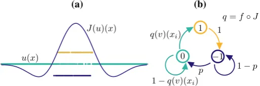
We use the termstochastic modelwhen the Markov chain model described below is posed onSN. An example of a state supported by the stochastic model is given in

Fig.1a.

In the model, neurons are coupled via a translation-invariant synaptic kernel, that is, we assume the connection strength between two neurons to be dependent on their mutual Euclidean distance. In particular, we prescribe that short range connections are excitatory, whilst long-range connections are inhibitory. To model this coupling, we use a standard Mexican hat function,

w:X→R, x→A1

B1/Lexp(−4B1x2)−A2

B2/Lexp(−4B2x2), (1)

(b) (a)

1

−1 0

1−p

1

p u(x)

q(v)(xi)

1−q(v)(xi)

J(u)(x)

q=f◦J

Fig. 1 aExample of a stateu(x)∈UNand corresponding synaptic profileJ(u)(x)∈RNin a stochastic network of 1024 neurons.bSchematic of the transition kernel for the network (see also Eqs. (5)–(7)). The conditional probability of thelocalvariableu(xi,t+1)depends on theglobalstate of the network at time

t, via the functionq= f◦J, as seen in (7)

In order to describe the dynamics of the model, it is useful to partition the tissueX into the 3 pullback sets

X_ku(t)= {x∈X:u(x,t)=k}, k∈U, t ∈Z, (2)

so that we can write, for instance, Xu₁(t)to denote the set of neurons that are firing at timet(and similarly for Xu₋₁andX₀u). Where it is unambiguous, we shall simply writeXkorXk(t)in place ofXuk(t).

The synaptic input to a cell at positionxiis given by a weighted sum of inputs from

all firing cells. Using the synaptic kernel (1) and the partition (2), the synaptic input is then modelled as

J :X×Z→R, (x,t)→κ

XW(x−y)1X1(t)(y)dy=κ

X1(t)

W(x−y)d y, (3) whereκ ∈ R₊is the synaptic gain, which is common for all neurons and1X is the

indicator function of a setX.

Remark 1 (Dependence of J on u) Since X1depends on the state variable u, so does the synaptic input(3). Where necessary, we will write J(u)(x,t)to highlight the dependence on u. We refer the reader to Fig.1for a concrete example of synaptic profile.

The firing probability associated to a quiescent neuron is linked to the synaptic input via the firing rate function

f :R→R, I → 1

1+exp[−β(I−h)], (4)

Pru(xi,t+1)= −1u(x,t)=v(x)

=

⎧ ⎪ ⎨ ⎪ ⎩

1−p ifv(xi)= −1,

1 ifv(xi)=1,

0 otherwise,

(5)

Pru(xi,t+1)=0u(x,t)=v(x)

=

⎧ ⎪ ⎨ ⎪ ⎩

p ifv(xi)= −1,

1− f(J(v))(xi) ifv(xi)=0,

0 otherwise,

(6)

Pru(xi,t+1)=1u(x,t)=v(x)

=

f(J(v))(xi) ifv(xi)=0,

0 otherwise, (7)

wherep∈(0,1]. We give a schematic representation of the transitions of each neuron in the network in Fig.1b. We remark that conditional probability of thelocalvariable u(xi,t+1)depends on theglobalstate of the network at timet, via the function f◦J.

The model described by (1)–(7), complemented by initial conditions, defines a stochastic evolution map that we will formally denote as

u(x,t+1)=ϕ(u(x,t);γ ), (8)

whereγ =(κ, β,h,p,A1,A2,B1,B2)is a vector of control parameters.

Remark 2 (Microscopic, mesoscopic and macroscopic descriptions) We will hence-forth use the terms “microscopic”, “mesoscopic” and “macroscopic” to refer to different state variables or model descriptions. Examples of these three state variables appear together in Figs.2,3and4in Sect.3, and we introduce them briefly here:

Microscopic level Model(8)will be referred to as microscopic model and its solu-tions at a fixed time t as microscopic states. We will use these terms also when p=1andβ → ∞, that is, when the evolution Eq.(8)is deterministic.

Mesoscopic level In Remark1, we associated to each microscopic state u a corre-sponding synaptic profile J , which is smooth, even when the tissue is discrete. We will not seek an evolution equation for the variable J , as the corresponding dynamical system would not reprent a reduction of the microscopic one. However, we will use J to bridge between the microscopic and macroscopic model descriptions; we therefore refer to J as a mesoscopic variable (or mesoscopic state).

Macroscopic level Much of the present paper aims to show that, for the model under consideration, there exists a high-level model description, in the spirit of interfacial dynamics for neural fields(Bressloff 2012;

Coombes et al. 2012; Bressloff 2014). The state variables for this level are points on the tissue where J(u)(x,t)attains the fir-ing rate threshold h. We will denote these threshold crossfir-ings as {ξi(t)}and we will discuss (reduced) evolution equations in terms

ofξi(t). The variables{ξ(t)}are therefore referred to as

(a)

x

−π π

u(x,50) J(x,50)

5

0

0

t

0

t

100 100

0

−1 3.5

(b)

x

−π π −π x π

ξ1 ξ2

J

−1 0 1 u

Fig. 2 Bump obtained via time simulation of the stochastic model for(x,t)∈ [−π, π] × [0,100].aThe microscopic stateu(x,t)(left) attains the discrete values−1 (blue), 0 (green) and 1 (yellow). The corre-sponding synaptic profileJ(x,t)is a continuous function. A comparison betweenJ(x,50)andu(x,50)is reported on the right panel, where we also mark the interval[ξ1, ξ2]whereJis above the firing threshold

h.bSpace-time plots ofuandJ. Parameters as in Table1

3 Microscopic states observed via direct simulation

In this section, we introduce a few coherent states supported by the stochastic model. The main aim of the section is to show examples of bumps, multiple bumps and trav-elling waves, whose existence and stability properties will be studied in the following sections. In addition, we give a first characterisation of the macroscopic variables of interest and link them to the microscopic structure observed numerically.

3.1 Bumps

In a suitable region of parameter space, the microscopic model supports bump solu-tions (Qi and Gong 2015) in which the microscopic variableu(x,t)is nonzero only in a localised region of the tissue. In thisactiveregion, neurons attain all values in

(a)

0

t

0

t

100 100

(b)

x

0

−2 5 J

−2π 2π−2π x 2π

−2 0 2

−2π ξ1 ξ2 . . . ξ7 ξ82π

−1 0 1 u

Fig. 3 Multiple bump solution obtained via time simulation of the stochastic model for (x,t) ∈

[−2π,2π] × [0,100].aThe microscopic stateu(x,t)in the active region (left) is similar to the one found for the single bump (see Fig.2a). A comparison betweenJ(x,50)andu(x,50)is reported on the right panel, where we also mark the intervals[ξ1, ξ2], . . . ,[ξ7, ξ8]whereJis above the firing thresholdh. bSpace-time plots ofuandJ. Parameters are as in Table1

of a localised region, in whichu(xi,0)are sampled randomly fromU. After a short

transient, a stochasticmicroscopicbump is formed. As expected due to the stochastic nature of the system (Kilpatrick and Ermentrout 2013), the active region wanders while remaining localised. A space-time section of the active region reveals a characteristic random microstructure (see Fig.2a).

By plotting J(x,t), we see that the active region is well approximated by the portion of the tissueX_≥= [ξ1, ξ2]where Jlies above the thresholdh. A quantitative

comparison between J(x,50) andu(x,50)is made in Fig. 2a. We interpret J as a mesoscopic variable associated with the bump, and ξ1 andξ2 as corresponding macroscopicvariables (see also Remark2).

3.2 Multiple-bumps solutions

0 5

0

−2 5

(a)

(b)

50

0

t

50

0

t

−π π

J J(x,45)

u(x,45)

x

−π π−π x π

ξ1 x ξ2

−1 0 1 u

Fig. 4 Travelling wave obtained via time simulation of the stochastic model for(x,t)∈ [−π, π]×[0,50]. aThe microscopic stateu(x,t)(left) has a characteristic microstructure, which is also visible on the right panel, where we compareJ(x,45)andu(x,45). As in the other cases, we mark the interval[ξ1, ξ2]where

Jis above the firing thresholdh.bSpace-time plots ofuandJ. Parameters are as in Table1

bump case (see Fig.3a). At the mesoscopic level, the set for which Jlies above the thresholdh is now a union of disjoint intervals[ξ1, ξ2], . . . ,[ξ7, ξ8]. The number of

bumps of the pattern depends on the width of the tissue; the experiment of Fig.3is carried out on a domain twice as large as that of Fig.2. The examples of bump and multiple-bump solutions reported in these figures are obtained for different values of the main control parameterκ(see Table1), however, these states coexist in a suitable region of parameter space, as will be shown below.

3.3 Travelling waves

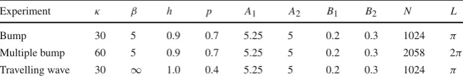
Table 1 Parameter values for which the stochastic model supports a bump (Fig.2), a multiple-bump solution (Fig.3) and a travelling wave (Fig.4).

Experiment κ β h p A1 A2 B1 B2 N L

Bump 30 5 0.9 0.7 5.25 5 0.2 0.3 1024 π

Multiple bump 60 5 0.9 0.7 5.25 5 0.2 0.3 2058 2π

Travelling wave 30 ∞ 1.0 0.4 5.25 5 0.2 0.3 1024 π

The value∞for the parameterβindicates that a Heaviside firing rate has been used in place of the sigmoidal function (4)

u(x,0)=

k∈U

k1Xk(x) with partition

X−1= [−1.5,−0.5),

X0= [−π,−1.5)∪ [0.5, π), X1= [−0.5,0.5).

In passing, we note that the state of the network at each discrete timet is defined entirely by the partition{Xk}of the tissue; we shall often use this characterisation in

the reminder of the paper.

In the direct simulation of Fig.4, the active region moves to the right and, after just 4 iterations, a travelling wave emerges. The microscopic variable,u(x,t), displays stochastic fluctuations which disappear at the level of the mesoscopic variable,J(x,t), giving rise to a seemingly deterministic travelling wave. A closer inspection (Fig.4a) reveals that the state can still be described in terms of the active region[ξ1, ξ2]where Jis aboveh. However, the travelling wave has a different microstructure with respect to the bump. Proceeding from right to left, we observe:

1. A region of the tissue ahead of the wave,x ∈(ξ2, π), where the neurons are in the

quiescent state 0 with high probability.

2. An active region x ∈ [ξ1, ξ2], split in three subintervals, each of approximate

width(ξ2−ξ1)/3, whereuattains with high probability the values 0, 1 and−1

respectively.

3. A region at the back of the wave,x∈ [−π, ξ1), where neurons are either quiescent

or refractory. We note thatu =0 with high probability asx → −π whereas, as x→ξ1, neurons are increasingly likely to be refractory, withu = −1.

A further observation of the space-time plot ofuin Fig.4b reveals a remarkably simple advection mechanism of the travelling wave, which can be fully understood in terms of the transition kernel of Fig.1b upon noticing that, for sufficiently large

β,qi = f(J(u))(xi) ≈ 0 everywhere except in the active region, whereqi ≈ 1.

(a) (b)

1

−1 0

1−p p

1

−1 0

1−p p

x∈[ξ1, ξ2]

x∈[ξ1, ξ2]

time t

ξ1(t) ξ2(t)

timet+ 1

ξ2(t+ 1)

ξ1(t+ 1)

0 1 −1 0

−1 1 0

0

1 0

−1 0

−1 0

0 −1

Fig. 5 Schematic of the advection mechanism for the travelling wave state. Shaded areas pertain to the active region[ξ1(t), ξ2(t)], non-shaded areas to the inactive regionX\[ξ1(t), ξ2(t)].aIn the active (inactive) region,qi= f(J(u))(xi)≈1 (qi ≈0), hence the transition kernel (5)–(7) can be simplified as shown.b At timetthe travelling wave has a profile similar to the one in Fig.4, which we represent in the proximity of the active region. We depict 5 intervals of equal width, 3 of which form a partition of[ξ1(t), ξ2(t)]. Each interval is mapped to another interval at timet+1, following the transition rules sketched in (a). In one discrete step, the wave progresses with positive speed: so thatJ(x,t+1)is a translation ofJ(x,t)

1. At the front of the wave, to the right ofξ2(t), neurons in the quiescent state 0

remain at 0 (rules forx∈ [/ ξ1, ξ2]).

2. Inside the active region, to the left ofξ2(t), we follow the rules for x ∈ [ξ1, ξ2]

in a clockwise manner: neurons in the quiescent state 0 spike, hence their state variable becomes 1; similarly, spiking neurons become refractory. Of the neurons in the refractory state, those being the ones nearestξ1(t), a proportion pbecome

(a)

(b)

(c)

0 t 100

1 3.5

Δ

0.6 1.8

0 t 100

Δ2

Δ1 Δ3

Δ4

0 t

1.2 1.6

Δ Δi

50

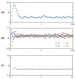
Fig. 6 Width of the active regionsΔi=ξ2i−ξ2i−1for the patterns in Figs.2,3and4.aBump, for which

i=1.bMultiple Bump,i =1, . . . ,4.cTravelling wave,i =1. In all cases, the patterns reach a coarse equilibrium state after a short transient

3. At the back of the wave, to the left ofξ1(t), the interval contains a mixture of

neurons in states 0 and−1. The former remain at 0 whilst, of the latter, a proportion ptransition into state 0, with the rest remaining at−1 (rules forx∈ [/ ξ1, ξ2]). From

this argument, we see that the proportion of refractory neurons in the back of the wave must decrease asξ → −π.

The resulting mesoscopic variable J(x,t+1)is a spatial translation by(ξ2(t)−

ξ1(t))/3 ofJ(x,t). We remark that the approximate transition rules of Fig.5a are valid

also in the case of a bump, albeit the corresponding microstructure does not allow the advection mechanism described above.

3.4 Macroscopic variables

The computations of the previous sections suggest that, beyond the mesoscopic vari-able, J(x), coarser macroscopic variables are available to describe the observed patterns. In analogy with what is typically found in neural fields with Heaviside fir-ing rate (Amari 1977; Bressloff 2014; Coombes and Owen 2004), the scalars{ξi}

defining the active region X_≥ = ∪i[ξ2i₋1, ξ2i], whereJ is aboveh, seem plausible

[ξ1(t+1), ξ2(t+1)]of the same width. To explore this further, we extract the widths

Δi(t)of each sub-interval[ξ2i(t), ξ2i−1(t)]from the data in Figs.2,3and4, and plot

the widths as a function oft. In all cases, we observe a brief transient, after which

Δi(t)relaxes towards a coarse equilibrium, though fluctuations seem larger for the

bump and multiple bump when compared with those for the wave. In the multiple bump case, we also notice that all intervals have approximately the same asymptotic width (see Fig.6b).

4 Deterministic model

We now introduce a deterministic version of the stochastic model considered in Sect. 2.2, which is suitable for carrying out analytical calculations. We make the following assumptions:

1. Continuum neural tissue.We consider the limit of infinitely many neurons and pose the model onS.

2. Deterministic transitions.We assume p=1, which implies a deterministic tran-sition from refractory states to quiescent ones (see Eq. (5)), andβ → ∞, which induces a Heaviside firing rate f(I)= (I−h)and hence a deterministic transi-tion from quiescent states to spiking ones given sufficiently high input (see Eqs.4,

6).

In addition to the pullback setsX₋1,X0, andX1defined in (2), we will partition

the tissue intoactiveandinactiveregions

X_≥(t)= {x∈X: J(x,t)≥h}, X_<(t)=X\X_≥(t). (9)

In the deterministic model, the transitions (5)–(7) are then replaced by the following rule

u(x,t+1)=

⎧ ⎪ ⎨ ⎪ ⎩

−1 ifx∈ X1(t),

0 ifx∈ X₋1(t)∪

X0(t)∩X<(t)

,

1 ifx∈ X0(t)∩X≥(t).

(10)

We stress that the right-hand side of the equation above depends onu(x,t), since the partitions{X₋1,X0,X1}and{X_<,X_≥}do so (see Remark1).

As we shall see, it is sometimes useful to refer to the induced mapping of the pullback sets

X₋1(t+1)=X1(t) X0(t+1)=X−1(t)∪

X0(t)∩X<(t)

X1(t+1)=X0(t)∩X≥(t)

. (11)

Henceforth, we will use the termdeterministic modeland formally write

u(x,t+1)=Φd(u(x,t);γ ). (12)

for (10), where the partition{Xk}k∈Uis defined by (2) and the active and inactive sets

ξ2m

ξm1

η1 η2

Am3 Am6 Am9 . . . Am3m h

Jm(x, η1, η2)

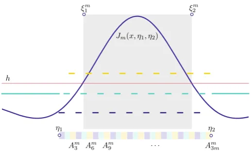
Fig. 7 Schematic of the analytical construction of a bump. A microscopic state whose partition comprises 3m+2 strips is considered. The microscopic state, which is not an equilibrium of the deterministic system, has a characteristic widthη2−η1, which differs from the widthξ2m−ξ1mof the mesoscopic bumpJm. If we letm→ ∞while keepingη2−η1constant, thenJmtends towards a mesoscopic bumpJbandξim→ηi (see Proposition1)

5 Macroscopic bump solution of the deterministic model

We now proceed to construct a bump solution of the deterministic model presented in Sect.4. In order to do so, we consider a microscopic state with a regular structure, resulting in a partition,{X_km}k, with 3m+2 strips (see Fig.7) and then study the limit

m→ ∞.

5.1 Bump construction

Starting from two points η1, η2 ∈ S, withη1 < η2, we construct 3m intervals as

follows

Ami =

η1+ i−1

3m (η2−η1), η1+ i

3m(η2−η1)

, i=1, . . . ,3m, m∈N. (13)

We then consider statesum(x)=k_∈Uk1Xm_k(x), with partitions given by

X₋m₁=

m

j=1

Am_3j−2, Xm₀ = [−L, η1)∪ [η2,L)

m

j=1

Am_3j−1, Xm₁ =

m

j=1

Am_3j, (14)

and activity setX_≥= [ξ₁m, ξ₂m]. We note that, in addition to the 3mstrips that form the active region of the bump, we also need two additional strips in the inactive region to form a partition ofS. In general,{ξ_im}i = {ηi}i, as illustrated in Fig.7. Applying (10)

or (11), we findΦd(um)=um, henceumare not equilibria of the deterministic model.

Jm(x, η1, η2)=κ

Xm₁(η1,η2)

W(x−y)dy, (15)

where we have highlighted the dependence ofX₁m onη1, η2. The proposition below

shows that there is a well defined limit,Jb, of the mesoscopic profile asm→ ∞. We

also have thatξ_im →ηi asm→ ∞and that the threshold crossings of the activity set

are roots of a simple nonlinear function.

Proposition 1 (Bump construction) Let W be the periodic extension of the synaptic kernel(1)and let h, κ∈R₊. Further, let{Am_i }_i3₌m₁, Xm₁ and Jmbe defined as in(13),

(14)and(15), respectively, and let Jb:S3→Rbe defined as

Jb(x, η1, η2)= κ

3

_η2

η1

W(x−y)d y.

The following results hold

1. Jm(x, η1, η2) → Jb(x, η1, η2)as m → ∞uniformly in the variable x for all

η1, η2∈Swithη1< η2,

2. If there existsΔ∈(0,L)such that3h=κ₀ΔW(y)d y, then Jb(0,0, Δ)= Jb(Δ,0, Δ)=h.

Proof We fix η1 < η2 and consider the 2L-periodic continuous mapping x → Jb(x, η1, η2), defined on S. We aim to prove that Jm → Jb uniformly in S. We

pose

I₋m₁(x)=

m

j=1

A3j−2

W(x−y)dy,

I₀m(x)=

m

j=1

A3j−1

W(x−y)dy,

I₁m(x)=

m

j=1

A3j

W(x−y)dy,

for allx∈S,m∈N. Since the intervals{Am_i }3_i=m₁form a partition of[η1, η2)we have

3

κJb(x)=I₋m1(x)+I

m

0(x)+I

m

1 (x) for allx∈S,m∈N. (16)

Since W is continuous on the compact setS, it is also uniformly continuous onS. Hence, there exists a modulus of continuityωofW:

ω(r)= sup

p,q∈S

|p−q|≤r

|W(p)−W(q)|, with lim

We useωto estimate|I₁m(x)−I₀m(x)|as follows:

|I₁m(x)−I₀m(x)| ≤ m

j=1 _A

3j

W(x−y)d y−

A3j−1

W(x−y)d y

=

m

j=1

η1+33mj(η2−η1)

η1+3₃j−_m1(η2−η1)

W(x−y)d y−

_η1+3j−1 3m (η2−η1)

η1+3₃j−_m2(η2−η1)

W(x−y)d y

=

m

j=1

η1+33mj(η2−η1)

η1+33j−m1(η2−η1)

W(x−y)−W

x−y+η2−η1 3m d y ≤ m

j=1 _η1+3j

3m(η2−η1)

η1+33j−m1(η2−η1)

W(x−y)−W

x−y+η2−η1 3m d y ≤ m

j=1 _η1+3j

3m(η2−η1)

η1+33j−m1(η2−η1)

ω

η2−η1

3m

d y

=ω

η2−η1

3m

η2−η1

3 .

We have then|I₁m(x)−I₀m(x)| →0 asm → ∞and sinceω(η2−η1)/(3m)

is independent ofx, the convergence is uniform. Applying a similar argument, we find |I₋m₁(x)−I₀m(x)| →0 asm→ ∞and using (16), we concludeI₁m,I₀m,I₋m₁→ Jb/κ

asm→ ∞. SinceI₁m= Jm/κ, thenJm → Jbuniformly for allx∈Sandη1, η2∈S

withη1< η2, that is, result 1 holds true.

By hypothesisJb(0,0, Δ)=hand, using a change of variables under the integral

and the fact thatWis even, it can be shown thatJb(Δ,0, Δ)=h, which proves result

2.

Corollary 1 (Bump symmetries)LetΔbe defined as in Proposition1, then Jb(x+

δ, δ, δ+Δ)is a mesoscopic bump for allδ ∈ [L,−Δ+L). Such bump is symmetric with respect to the axis x =δ+Δ/2.

Proof The assertion is obtained using a change of variables in the integral definingJb

and noting thatW is even.

The results above show that,ξ_im → ηi asm → ∞, hence we lose the distinction

between width of the microscopic pattern, η2 −η1, and width of the mesoscopic

pattern,ξ₂m−ξ₁m, in that result 2 establishesJb(ηi, η1, η2)=h, forη1=0,η2=Δ.

With reference to Fig.7, the factor 1/3 appearing in the expression for Jbconfirms

that, in the limit of infinitely many strips, only a third of the intervals{Am_j}jcontribute

to the integral. In addition, the formula for Jbis useful for practical computations as

it allows us to determine the width,Δ, of the bump.

Remark 3 (Permuting intervals Am_i ) A bump can also be found if the partition{Xm_k} of umis less regular than the one depicted in Fig.7. In particular, Proposition1can be

permutations,σj, of the index sets{3j−2,3j−1,3j}for j=1, . . . ,m and construct

partitions

X₋m₁=

m

j=1 Am_σ

j(3j−2), X

m

0 = [−L,0)∪ [Δ,L)

m

j=1 Am_σ

j(3j−1), X

m

1 =

m

j=1 Am_σ

j(3j),

then the resulting Jm converges uniformly to Jbas m → ∞. The proof of this result follows closely the one of Proposition1and is omitted here for simplicity.

5.2 Bump stability

Once a bump has been constructed, its stability can be studied by employing standard techniques used to analyse neural field models (Bressloff 2012). We consider the map

b:S2×S2→R2, (ξ, η)→

Jb(ξ1, η1, η2)−h Jb(ξ2, η1, η2)−h

.

and study the implicit evolution

b(ξ(t+1), ξ(t))=0. (17)

The motivation for studying this evolution comes from Proposition 1, accord-ing to which the macroscopic bumpξ∗ =(0, Δ)is an equilibrium of (17), that is,

b(ξ∗, ξ∗) =0. To determine coarse linear stability, we study how small

perturba-tions ofξ_∗evolve according to the implicit rule (17). We setξ(t)=ξ_∗+εξ(t), for 0 < 1 withξi =O(1)and expand (17) around(ξ∗, ξ∗), retaining terms up to

orderε,

b(ξ∗+εξ(t+1), ξ∗+εξ(t))=b(ξ∗, ξ∗)+εDξb(ξ∗, ξ∗)ξ(t+1)

+εD_ξb(ξ∗, ξ∗)ξ(t).

Using the classical ansatzξ(˜ t)=λtv, withλ∈Candv∈S2, we obtain the eigenvalue problem

λ

v1

v2

= 1

W(0)−W(Δ)

−W(0) W(Δ) W(Δ) −W(0)

v1

v2

, (18)

with eigenvalues and eigenvectors given by

λ1=

W(Δ)−W(0)

W(0)−W(Δ) = −1, v 1₌₍

1,1)T,

λ2=−

W(0)−W(Δ)

W(0)−W(Δ) , v

2_=(−1,

1)T.

compression/extension eigenvector, determines the stability of the macroscopic bump. The parametersAi,Biin Eq. (1) are such thatWhas a global maximum atx =0, with

W(0) >0. Hence, the eigenvalues are finite real numbers and the pattern is stable if W(Δ) <0. We will present concrete bump computations in Sect.10.

5.3 Multi-bump solutions

The discussion in the previous section can be extended to the case of solutions featuring multiple bumps. For simplicity, we will discuss here solutions with 2 bumps, but the case ofkbumps follows straightforwardly. The starting point is a microscopic structure similar to (14), with two disjoint intervals[η1, η2),[η3, η4)⊂Seach subdivided into

3msubintervals. We form the vectorη= {ηi}4i=1and have

κ

Xm₁

W(x−y)d y= 2

j=1

Jm(x, η2j−1, η2j)→

2

j=1

Jb(x, η2j−1, η2j),

asm→ ∞uniformly in the variablexfor allη1, . . . , η4∈Swithη1< . . . < η4. In

the expression above,JmandJbare the same functions used in Sect.5.1for the single

bump. In analogy with what was done for the single bump, we consider the mapping defined by

:S4_×S4_→R4_{, (ξ, η)→}

−h+ 2

j=1

Jb(ξi, η2j−1, η2j)

4

i₌1

.

Multi-bump solutions can then be studied as in Sect.5. We present here the results for a multi-bump forL=πwith threshold crossings given by

ξ∗= 1₂ ⎡ ⎢ ⎢ ⎣

−π−Δ

−π+Δ π−Δ π+Δ

⎤ ⎥ ⎥

⎦, (19)

whereΔsatisfies

Jb

π+Δ

2 ,

−π−Δ

2 ,

−π+Δ

2

+Jb

π+Δ

2 ,

π−Δ

2 ,

π+Δ

2

=h. (20)

A quick calculation leads to the eigenvalue problem

λ ⎡ ⎢ ⎢ ⎣ v1 v2 v3 v4 ⎤ ⎥ ⎥ ⎦= _α1

⎡ ⎢ ⎢ ⎣

W(0) −W(Δ) W(π) −W(π−Δ)

−W(Δ) W(0) −W(π−Δ) W(π)

W(π) −W(π−Δ) W(0) −W(Δ)

−W(π−Δ) W(π) −W(Δ) W(0)

4

−2

−π ξ1 ξ2 0 ξ3 ξ4 π

v2 v1

v3

v4

x J

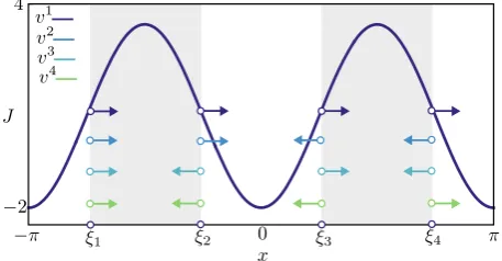
Fig. 8 Stable mesoscopic multi-bump obtained for the deterministic model. We also plot the corresponding macroscopic bumpξ∗(Eqs.19–20) and coarse eigenvectors. Parameters areκ =30,h = 0.9,p =1, β→ ∞, with other parameters as in Table1

whereα = −W(0)+W(Δ)−W(π)+W(π−Δ). The real symmetric matrix in Eq. (21) has eigenvalues and eigenvectors given by

λ1= −

W(0)+W(Δ)−W(π)+W(π−Δ)

W(0)−W(Δ)+W(π)−W(π−Δ) = −1, v 1₌₍

1,1,1,1)T,

λ2= −

W(0)+W(Δ)+W(π)−W(π−Δ)

W(0)−W(Δ)+W(π)−W(π−Δ) , v 2₌₍

1,1,−1,−1)T,

λ3= −

W(0)−W(Δ)−W(π)−W(π−Δ)

W(0)−W(Δ)+W(π)−W(π−Δ) , v 3₌₍

1,−1,1,−1)T,

λ4= −

W(0)−W(Δ)+W(π)+W(π−Δ)

W(0)−W(Δ)+W(π)−W(π−Δ) , v 4₌₍

1,−1,−1,1)T.

As expected, we have one neutral translational mode. If the remaining 3 eigenvalues lie in the unit circle, the multi-bump solution is stable. A depiction of this multi-bump, with corresponding eigenmodes can be found in Fig.8. We remark that the multi-bump presented here was constructed imposing particular symmetries (the pattern is even; bumps all have the same widths). The system may in principle support more generic bumps, but their construction and stability analysis can be carried out in a similar fashion.

6 Travelling waves in the deterministic model

Travelling waves in the deterministic model can also be studied via threshold crossings, and we perform this study in the present section. We seek a measurable function utw :S→Uand a constantc∈Rsuch that

u(x,t)=utw(x−ct)=

k∈U

k1_Xtw

almost everywhere inSand for allt ∈ Z. We recall that, in general, a stateu(x,t) is completely defined by its partition,{X_ktw(t)}. Consequently, Eq. (22) expresses that a travelling wave has a fixed profileutw, whose partition,{Xtw_k }, does not depend on

time. A travelling wave(utw,c)satisfies almost everywhere the condition

utw =σ−cΦd(utw;γ ),

whereΦdis the deterministic evolution operator (12) and the shift operator is defined

byσx : u(·)→ u(· −x). The existence of a travelling wave is now an immediate

consequence of the symmetries of W, as shown in the following proposition. An important difference with respect to the bump is that analytical expressions can be found for both microscopic and mesoscopic profiles, as opposed to Proposition 1, which concerns only the mesoscopic profile.

Proposition 2 (Travelling wave) Let h, κ∈R₊. If there existsΔ∈(0,L)such that h =κ_Δ2ΔW(y)d y, then

utw(z)=

k_∈U

k1Xtw

k (z), with partition

Xtw₋1= [−2Δ,−Δ),

Xtw₀ = [−L,−2Δ)∪ [0,L), Xtw₁ = [−Δ,0),

is a travelling wave of the deterministic model(12)with speed c = Δ, associated mesoscopic profile Jtw(z)=κ

0

−ΔW(z−y)dy and activity set Xtw≥ = [−2Δ, Δ]. Proof The assertion can be verified directly. We have

h

κ =

2Δ

Δ w(y)d y= 0

−ΔW(Δ−y)d y= 0

−ΔW(−2Δ−y)d y,

hence the activity set forutwisXtw_≥ = [−2Δ, Δ]with mesoscopic profileκ 0

−ΔW(z− y)dy. Consequently,Φd(utw;γ )has partition

Y₋1= [−Δ,0),

Y0= [−L,−Δ)∪ [Δ,L), Y1= [0, Δ],

andutw=σ−ΔΦd(utw, γ )almost everywhere.

Numerical simulations of the deterministic model confirm the existence of the mesoscopic travelling waveutw in a suitable region of parameter space, as will be

(b) (a)

t= 1

t= 30

t= 49

0.03

0.004

0.003

0.01 0.01

σ−tΔΦd(utw+ε˜u), κ= 38 σ−tΔΦd(utw+εu˜), κ= 33

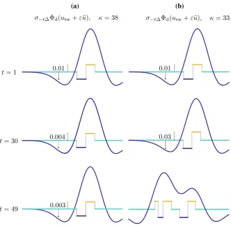
Fig. 9 Numerical investigation of the linear stability of the travelling wave of the deterministic system, subject to perturbations in the wake of the wave. We iterate the mapΦdstarting from a perturbed state

utw+εu˜, whereutwis the mesoscopic wave profile of Proposition2, travelling with speedΔ, andεu˜is non-zero only in two intervals of width 0.01 in the wake of the wave. We plotσ₋tΔΦd(utw+εu˜)and the corresponding macroscopic profile as a function oftand we annotate the width of one of the perturbations. aForκ=38, the wave is stable.bfor sufficiently smallκ, the wave becomes unstable

in Fig.4is in the wake of the wave, where the former features quiescent neurons and the latter a mixture of quiescent and refractory neurons.

6.1 Travelling wave stability

As we will show in Sect.10, waves can be found for sufficiently large values of the gain parameterκ. However, when this parameter is below a critical value, we observe that waves destabilise at their tail. This type of instability is presented in the numerical experiment of Fig.9. Here, we iterate the dynamical system

whereutwis the profile of Proposition2, travelling with speedΔ, and the perturbation

εutw is non-zero only in two intervals of width 0.01. We deem the travelling wave

stable ifu(z,t)→utw(z)ast → ∞. Forκsufficiently large, the perturbations decay,

as witnessed by their decreasing width in Fig.9a. Forκ =33, the perturbations grow and the wave destabilises.

To analyse the behaviour of Fig.9, we shall derive the evolution equation for a relevant class of perturbations toutw. This class may be regarded as a generalisation

of the perturbation applied in this figure and is sufficient to capture the instabilities observed in numerical simulations. We seek solutions to (23) with initial condition u(z,t)=_kk1Xk(t)(z)with time-dependent partitions

X₋1(t)=

−4Δ+δ1(t),−4Δ+δ2(t) ∪

−2Δ+δ5(t),−Δ+δ6(t) , X0(t)=

−L,−4Δ+δ1(t) ∪

−4Δ+δ2(t),−3Δ+δ3(t)

∪−3Δ+δ4(t),−2Δ+δ5(t) ∪

δ7(t),L , X1(t)=

−3Δ+δ3(t),−3Δ+δ4(t) ∪

−Δ+δ6(t), δ7(t) ,

and activity set X_≥(t) = [ξ1(t), ξ2(t)]. In passing, we note that for δi = 0, the

partition above coincides with{Xtw_k }in Proposition2, hence this partition can be used as perturbation ofutw. Inserting the ansatz foru(ξ,t)into (23), we obtain a nonlinear

implicit evolution equation,δ(t+1), δ(t)=0, for the vectorδ(t)as follows (see Fig.10)

δ1(t+1)=δ3(t),

δ2(t+1)=δ4(t), ₋3Δ+δ4(t)

−3Δ+δ3(t)

w(−2Δ+δ3(t+1)−y)d y+ _δ7(t)

−Δ+δ6(t)

w(−2Δ+δ3(t+1)−y)d y=h/κ,

δ4(t+1)=δ5(t),

δ5(t+1)=δ6(t),

δ6(t+1)=δ7(t), ₋3Δ+δ4(t)

−3Δ+δ3(t)

w(Δ+δ7(t+1)−y)d y+ _δ7(t)

−Δ+δ6(t)

w(Δ+δ7(t+1)−y)d y=h/κ.

We note that the map above is valid under the assumptionδ3(t) < δ4(t), which

preserve the number of intervals of the original partition. As inKilpatrick and Bressloff

(2010), we note that this prevents us from looking at oscillatory evolution ofδ(t). We setδi(t)=ελtvi, retain terms up to first order and obtain an eigenvalue problem for

ξ1(t) ξ2(t)

δ1(t)

δ2(t)

δ3(t)

δ4(t)

δ6(t) δ7(t)

δ3(t)

δ4(t)

δ5(t)

δ6(t) δ7(t) ξ2−Δ

−4Δ −3Δ −2Δ −Δ 0 Δ 2Δ

δ2(t+ 1) =δ4(t)

δ1(t+ 1) =δ3(t)

δ5(t)

ξ1+ 2Δ

δ3(t+ 1) =ξ1+ 2Δ

δ4(t+ 1) =δ5(t)

δ5(t+ 1) =δ6(t) δ6(t+ 1) =δ7(t)

δ7(t+ 1) =ξ2−Δ

u(z, t)

Φd(u(z, t))

σ−ΔΦd(u(z, t))

1

α

⎡ ⎢ ⎢ ⎢ ⎢ ⎢ ⎢ ⎢ ⎢ ⎣

0 0 α 0 0 0 0

0 0 0 α 0 0 0

0 0−w(Δ) w(Δ) 0−w(Δ) w(2Δ)

0 0 0 0 α 0 0

0 0 0 0 0 α 0

0 0 0 0 0 0 α

0 0 w(4Δ) −w(4Δ) 0 w(2Δ) −w(Δ)

⎤ ⎥ ⎥ ⎥ ⎥ ⎥ ⎥ ⎥ ⎥ ⎦

,

whereα =w(2Δ)−w(Δ). Once again, we have an eigenvalue on the unit circle, corresponding to a neutrally stable translation mode. If all other eigenvalues are within the unit circle, then the wave is linearly stable. Concrete calculations will be presented in Sect.10.

7 Approximate probability mass functions for the Markov chain model

We have thus far analysed coherent states of a deterministic limit of the Markov chain model, and we now move to the more challenging stochastic setting. More precisely, we return to the original model (8) and findapproximatemass functions for the coherent structures presented in Sect.3(see Figs.2,3,4). These approximations will be used in the lifting procedure of the equation-free framework.

The stochastic model is a Markov chain whose 3N-by-3N transition kernel has entries specified by (1). It is useful to examine the evolution of the probability mass function for the state of a neuron at position xi in the network, μk(xi,t) =

Pru(xi,t)=k

,k∈U, which evolves according to

⎡

⎣μ_μ−01((xxii,,tt++11))

μ1(xi,t+1)

⎤ ⎦₌

⎡

⎣1−p p1− f(J(0u))(xi,t)10

0 f(J(u))(xi,t) 0

⎤ ⎦

⎡

⎣μ_μ−01((xxii,,tt))

μ1(xi,t)

⎤

⎦_, (24)

or in compact notationμ(xi,t+1)=(xi,t)μ(xi,t). We recall thatf is the sigmoidal

firing rate and thatJ is a deterministic function of the random vector,u(x,t)∈UN, via the pullback setXu₁(t):

J(u)(x,t)=κ

XW(x−y)1X

u

1(t)(y)dy.

As a consequence, the evolution equation for μ(xi,t)is non-local, in that J(xi,t)

depends on the microscopic state of the whole network.

We now introduce an approximate evolution equation, obtained by posing the prob-lem on a continuum tissueSand by substitutingJ(x,t)by its expected value

whereμ:S×Z→ [0,1]3,

(x,t)= ⎡

⎣1−p p1− fE0[J](x,t)10 0 fE[J](x,t) 0

⎤

⎦_, (26)

and

E[J](x,t)=κ

Sw(x−y)μ1(y,t)dy. (27) In passing, we note that the evolution Eq. (25) is deterministic. We are interested in two types of solutions to (25):

1. A time-independent bump solution, that is a mappingμbsuch thatμ(x,t)=μb(x)

for allx∈Sandt∈Z.

2. A travelling wave solution, that is, a mappingμtwand a real numbercsuch that

μ(x,t)=μtw(x−ct)for allx∈Sandt ∈Z.

7.1 Approximate probability mass function for bumps

We observe that, posingμ(y,t)=μb(y)in (25), we have

E[J](x)=κ

Sw(x−y)(μb)1(y)dy.

Motivated by the simulations in Sect. 3 and by Proposition1, we seek a solution to (25) in the limitβ → ∞, withE[J](x)≥hforx ∈ [0, Δ], and(μb)1(x)=0 for x∈ [0, Δ], whereΔis unknown. We obtain

μb(x)=b(x)μb(x),

where

b(x)= ⎡

⎣1−p p0 11 0

0 0 0

⎤

⎦_1S\[0,Δ](x)+ ⎡

⎣1−p p0 10 0

0 1 0

⎤

⎦_1[0,Δ](x)

=Q_<1_S\[0,Δ](x)+Q≥1[0,Δ](x),

We conclude that, for eachx∈ [0, Δ](respectivelyx ∈S\[0, Δ]),μb(x)is the right

· 1-unit eigenvector corresponding to the eigenvalue 1 of the stochastic matrixQ≥

(respectivelyQ_<). We find

μb(x)= ⎡ ⎣01

0

⎤

⎦_1S\[0,Δ](x)+ p 1+2p

⎡ ⎣1/1p

1

⎤

0 0

1

−2 _x 2 ₋₂ 0 ₂

x

μb μ1

μ0

μ-1 μ (b)

(a)

p= 1, β→ ∞ p= 0.7, β= 5

(c) (d)

4

5.3

3

5.2

2

5.1

1

1 δ 4

Δ∼Pr(δ)

4 5 .3 3

5.2

2 5 .1 1

1 δ 4

Δ∼Pr(δ)

Fig. 11 Comparison between the probability mass functionμb, as computed by (28)–(29), and the observed distributionμof the stochastic model.aWe compute the vector(μb)k,k∈Uin each strip using (30) and visualise the distribution using vertically juxtaposed color bars, with height proportional to the values (μb)k, as shown in the legend.bA long simulation of the stochastic model supporting a stochastic bump

u(x,t)fort ∈ [0,T], whereT =105. At each timet>10 (allowing for initial transients to decay), we computeξ1(t),ξ2(t),Δ(t)and then produce histograms for the random profileu(x−ξ1(t)−Δ(t)/2,t). cIn the deterministic limit, the value ofΔis determined by (29), hence we have a Dirac distribution.dthe distribution ofΔobtained in the Markov chain model. Parameters are as in Table1

and, by imposing the threshold conditionE[J](Δ) = h, we obtain a compatibility condition forΔ,

h = κp 1+2p

_Δ

0

w(Δ−y)dy. (29)

We note that ifp =1 we haveE[J](x)=Jb(x,0, Δ)where Jbis the profile for the

mesoscopic bump found in Proposition1, as expected.

In Fig.11a, we plotμb(x)as predicted by (28)–(29), forp =0.7, κ=30,h=0.9.

At eachx, we visualise(μb)k for eachk∈Uusing vertically juxtaposed color bars,

with height proportional to the values(μb)k, as shown in the legend. For a qualitative

comparison with direct simulations, we refer the reader to the microscopic profile u(x,50)shown in the right panel of Fig.2a: the comparison suggests that eachu(xi,50)

is distributed according toμb(xi).

We also compared quantitatively the approximate distribution μb with the

t, we compute the mesoscopic profile,J(u)(x,t), the corresponding threshold cross-ings and width:ξ1(t),ξ2(t),Δ(t)and then produce histograms for the random profile u(x−ξ1(t)−Δ(t)/2,t). The instantaneous shift applied to the profile is necessary

to pin the wandering bump.

We note a discrepancy between the analytically computed histograms, in which we observe a sharp transition between the regionx ∈ [0, Δ]andx ∈ S\[0, Δ], and the numerically computed ones, in which this transition is smoother. This discrep-ancy arises becauseΔ(t)oscillates around an average valueΔpredicted by (29); the approximate evolution Eq. (25) does not account for these oscillations. This is visible in the histograms of Fig.11c, d, as well as in the direct numerical simulation Fig.6a.

7.2 Approximate probability mass function for travelling waves

We now follow a similar strategy to approximate the probability mass function for travelling waves. We poseμ(x,t)=μtw(x−ct)in the expression forE[J], to obtain

κ

Sw(x−y)(μtw)1(y−ct)dy=κ

Sw(x−ct−y)(μtw)1(y)dy=E[J](x−ct). Proposition2provides us with a deterministic travelling wave with speedc=Δ. The parameterΔis also connected to the mesoscopic wave profile, which has threshold crossingsξ1 = −2Δandξ2 =Δ. Hence, we seek for a solution to (25) in the limit

β → ∞, withE[J](z)≥ hfor x ∈ [−2c,c], and(μtw)1(z)= 0 forz ∈ [−2c,c],

wherecis unknown. For simplicity, we pose the problem on a large domain whose size is commensurate withc, that isS = cT/R, where T is an even integer much greater than 1.

We obtain

σctμtw(z)=tw(z−c(t−1))tw(z−c(t−2))· · ·tw(z)μtw(z),

where

tw(z)=Q<1S_\[−c_,c_](z)+Q≥1S_[−2c_,c_](z).

To make further analytical progress, it is useful to partition the domainS=cT/R in strips of widthc,

S=

T/2

j=T/2

j c, (j+1)c=

T/2−1

j=T/2 Ij(c),

and impose that the wave returns back to its original position after T iterations,

σcTμtw(z)=μtw(z), while satisfying the compatibility conditionh=E[J](c). This