GENERATION AND NONLINEAR PROPAGATION OF
ULTRASHORT NEAR INFRARED LASER PULSES
Peter N. Kean
A Thesis Submitted for the Degree of PhD
at the
University of St Andrews
1990
Full metadata for this item is available in
St Andrews Research Repository
at:
http://research-repository.st-andrews.ac.uk/
Please use this identifier to cite or link to this item:
http://hdl.handle.net/10023/14317
Generation and Nonlinear Propagation of Ultrashort
Near Infrared Laser Pulses.
Thesis submitted for the degree of Doctor of Philosophy to the University of St. Andrews
by
Peter N. Kean, B.Sc.
Department of Physics and Astronomy University of St. Andrews
North Haugh St. Andrews, Fife Scotland. KY16 9SS
ProQuest Number: 10166836
All rights reserved
INFORMATION TO ALL USERS
The quality of this reproduction is dependent upon the quality of the copy submitted.
In the unlikely event that the author did not send a com plete manuscript and there are missing pages, these will be noted. Also, if material had to be removed,
a note will indicate the deletion.
uest
ProQuest 10166836
Published by ProQuest LLO (2017). Copyright of the Dissertation is held by the Author.
All rights reserved.
This work is protected against unauthorized copying under Title 17, United States C ode Microform Edition © ProQuest LLO.
ProQuest LLO.
789 East Eisenhower Parkway P.Q. Box 1346
Declaration.
I hereby certify that this thesis has been composed by myself, that it is a record of my own work and that it has not been accepted in partial or complete fulfilment of any other degree of professional qualification.
I was admitted to the Faculty of Science of the University of St. Andrews as a candidate for the degree of Ph.D under ordinance general no. 12 on October 1985.
Signed Date
Certificate.
I hereby certify that the candidate has fulfilled the conditions of the Resolution and Regulations appropriate to the degree of Ph.D.
Signature of Supervisory Date
Copyright
To my Parents.
Abstract
By utilising a CW mode-locked Nd:YAG pump laser an experimental study of self phase modulation (SPM) and stimulated Raman scattering (SRS) in single mode optical fibres has been conducted. The dependence of the spectral broadening due to SPM upon the launched optical power was observed to obey a linear relationship in agreement with a simple theory. A deviation from this occurred for high input powers due to the onset of stimulated Raman scattering which caused a preferential depletion of the leading edge of the pump pulse and an increased spectral broadening to the long wavelength side of the spectrum. The pulses exiting the fibre were then compressed using a pair of holographic diffraction gratings, which were able to compensate for the linear part of the frequency chirp imposed on the pulse by SPM and the 1.06 jim pulses were reduced in duration from ~ 100 ps to approximately 4 ps by this method.
By making use of Raman generation in the fibre, a synchronously pumped fibre Raman oscillator was constructed. This enabled the generation of frequency tunable (1.07-1.12 |xm) near infrared pulses by the method of time dispersion tuning. By incorporating two fibre grating reflectors onto the ends of the optical fibre, an all-fibre device was constructed having the potential advantages of compactness and stability.
The generation of mode-locked pulses around the 1.5 pm wavelength region was accomplished with the use of a colour centre laser based upon a stabilised centre in NaCl or a thallium centre in KCl. Both of these lasers were examined, although to date the poor quality of our NaCl laser crystals has meant that most of the work reported here was performed with KChTl. This laser produced pulses of = 20 ps duration, tunable over 1.45 - 1.55 pm with average powers « 200 mW. A simple experiment to observe soliton propagation of these pulses in an optical fibre was conducted and this compressed the pulses to » 0.8 ps, although this does not represent the optimum compression that could be achieved.
Contents.
Abstract
Chapter 1. General Introduction Page.
1.1 Historical Background and Introduction 1
1.2 Introduction to Mode-Locking 3
1.2.1 Active Mode-Locking 6
1.2.2 Passive Mode-Locking 8
1.3 Ultrashort Pulse Measurement Techniques 9 1.3.1 The Electron-Optical Streak Camera 9 1.3.2 The Second Harmonic Generation Autocorrelator 12 1.4 A Brief Review of the Guiding Properties of Optical Fibres 17
1.5 Conclusions 21
References 23
Chapter 2. The Acousto-Optically Mode-locked Nd:YAG Laser
2.1 Introduction 26
2.2 The Spectra-Physics Series 3000 Laser System 27
2.2.1 The Acousto-Optic Mode-Locker 29
2.3 Laser Performance and Characterisation 32
2.4 Conclusions 40
References 42
Chapter 3. Nonlinear Pulse Propagation in Optical Fibres 3.1 Introduction
3.2 Self-Phase Modulation (SPM) 3.2.1 Theory of SPM
3.2.2 Experimental Observation of SPM 3.3 Optical Pulse Compression
43 45 45 53
3.4 Stimulated Raman Scattering (SRS) 72 3.4.1 Effect of SRS on SPM and Pulse Compression 75
3.4.2 The Fibre Raman Oscillator 80
3.4.3 Fibre Raman Oscillator with Fibre Grating Reflectors 87
3.5 Conclusions 98
References 100
Chapter 4. The KC1;TI and NaCP.GH" Colour Centre Lasers
4.1 Introduction 103
4.2 Some Basic Physics of Laser-Active Colour Centres 105
4.3 The p2+ and (F2+)a Centres 110
4.4 The Stabilised F2+ Centre in NaCl 113
4.5 The TP(1) Centre in KCl 115
4.6 Colour Centre Laser Resonators 118
4.6.1 The Burleigh Colour Centre Laser 122 4.7 The Mode-Locked KC1:T1 Colour Centre Laser 127
4.8 The NaChOH" Colour Centre Laser 134
4.9 Conclusions 137
References 138
Chapter 5. Optical Sditons and the Soliton Laser
5.1 Introduction 140
5.2 A Derivation of the NLS for Nonlinear Pulse Propagation 143
5.3 Soliton Solutions to the NLS 146
5.4 Observation of Optical SoUtons 151
5.5 The Soliton Laser 154
5.6 Conclusions 160
Chapter 6. Coupled-Cavity Mode-Locking 6.1 Introduction
6.2 The Experimental System
6.3 The CCM Laser with Normally Dispersive Fibre 6,3.1 The LiF:p2+ Coupled-Cavity Laser
6.4 The CCM Laser with a Semiconductor Diode Amplifier 6.5 A Discussion of the CCM Process
6.6 Conclusions References
164
164 169 178 179 181 189 191
Chapter 7. General Conclusions References
192 197
Appendix.
Acknowledgements.
Publications.
198
199
Chapter 1.
General Introduction.
1.1 Historical Background and Introduction.
In the 1960's, soon after the development of the laser, much consideration was given to the production of short, intense pulses of light. It was realised that the large bandwidth of lasers gave them the potential to produce extremely short light pulses in the region of picoseconds (lO'^^ or femtoseconds (10-*^ s). The technique of mode-locking for producing such pulses was first described in papers by DiDomenico [1], Hargrove et al [2] and Yariv [3] and several experiments were performed on mode-locking the He-Ne laser [4,5]. As early as 1966 the Nd:YAG laser was mode-locked, producing ultrashort pulses in the infrared at 1.06 pm [6]. An early review paper on the theory of mode-locking by intracavity loss modulation was published by Harris [7]. It was demonstrated by Mocker and Collins [8] that a saturable dye in the laser cavity could also be used to mode-lock a laser. This important method of mode-locking has led to some of the shortest pulses ever produced in the colliding pulse mode-locked ring dye laser [9]. Mode-locking by intracavity loss or gain modulation, has become known as active mode-locking, while the use of saturable elements (dyes or multiple quantum wells) is known as passive mode- locking.
is of a continuous wave (CW) nature. This lead to DiDomenico et al [6] estimating » 80 ps for the pulse duration from the mode-locked Nd:YAG laser. Development of the second harmonic autocorrelator [10,11], described later in this chapter, now enables pulse durations of only a few femtoseconds to be measured. Unfortunately, because this measurement technique is a nonlinear autocorrelation of the pulses, information on the temporal profile of the pulse is lost and one has to assume a pulse shape. Linear measurement techniques such as fast photodiodes [12] and the electron-optical streak camera [13] overcome this disadvantage, although to-date their temporal resolution is not much better than 1 ps.
Ultrashort pulses in the near infrared (NIR) spectral region (roughly 800 nra to 5 pm) have become of major importance in many areas of physics, chemistry and biology. Such pulses are used in the study of ultrafast chemical dynamics, vibration dephasing times in excited molecules and in spectroscopy for the measurement of fluorescence rise and decay times [14,15]. Relaxation, diffusion and nonlinear processes may be studied in narrow band gap semiconductors and multiple quantum wells [16,17], A developing field is that of electro-optic sampling, where short light pulses are used to characterise and measure the response of electrical circuits [18]. Ultrashort pulses enable the direct measurement of processes in the time domain, shorter pulses enabling higher temporal resolution and is a complementary approach to measuring slow events in the frequency domain with narrow linewidth lasers. Perhaps one of the most exciting applications of ultrashort NIR pulses, is towards optical communications [19]. Communication via optical fibres enables much higher data rates to be achieved and all optical switches have the potential to be much faster than electrical methods. In this regard, much experimental and theoretical work has been conducted on the propagation of pulses in optical fibres and in chapter 3, a study of two major nonlinear effects of pulse propagation in optical fibres is presented
1.3 and 1.5 jim. Colour centre lasers have proved to be extremely useful sources of tunable NIR radiation. These solid state lasers, with similar optical properties to dyes, can provide infrared radiation over the 0.8 - 4 jim spectral range with average powers of hundreds of milliwatts [26]. Mode-locked colour centre lasers have produced subpicosecond pulses by synchronous and passive mode-locking at around 950 nm [27] and 870 nm [28] respectively, and the recent development of the 'soliton' laser, to be described in chapter 5, has enabled the production of 60 fs pulses at 1.5 jim [29].
My work for this thesis, has concentrated on the generation of frequency tunable, ultrashort optical pulses in the near infrared. The nonlinear propagation of pulses in optical fibres is one method by which this may be achieved through the process of stimulated Raman scattering (chapter 3), and a more direct approach using colour centre lasers is described in chapter 4. The marriage of these two (nonlinear pulse propagation and ultrashort pulse generation) is hopefully further demonstrated in chapters 5 and 6, with the introduction of the soliton laser and the discovery of the more general technique which we have termed coupled-cavity mode-locking. The remainder of this chapter is devoted to an introduction of ultrashort pulse generation via mode-locking, pulse measurement techniques and a brief overview of the guiding properties of optical fibres,
1.2 Introduction to Mode-locking.
Af = c/2L (1.1) where L is the optical path length of the resonator. Superimposed on top of this is the gain profile of the amplifying medium, which serves to both define the central operating wavelength of the laser and limit the number of longitudinal modes allowed to reach threshold. This situation is shown in figure lb.
a.
b.
H]
Allowed axial modeao Loss line
Frequency
[image:15.619.181.402.220.443.2]c.
Figure 1.
(a) A laser resonator containing the gain medium and showing a single longitudinal mode, (b) Gain profile imposed on the longitudinal modes of the resonator, allowing a limited number to reach laser threshold, (c) Temporal output of a mode-locked laser.
gain, which creates sidebands on each of the cavity modes. If the modulation period coincides with the cavity roundtrip time, the sidebands will overlap with an adjacent cavity mode and injection locking effects lead to strong mode coupling and cause phase-locking of the longitudinal modes. The greater the number of modes that are phase locked, the shorter the duration of each pulse and the peak intensity of each pulse is a factor of greater than that of any single mode, where N is the number of oscillating, phase locked, modes. An inhomogeneously broadened laser, such as many gas or ion lasers, will spontaneously oscillate on many longitudinal modes and mode-locking is easily achieved by applying sufficient modulation, enabling phase-locking to occur. In contrast, a homogeneously broadened laser, will normally oscillate on only one or at most, a few, longitudinal modes (due to spatial hole-burning effects) near the peak of the gain. In this case the mode-locker acts to transfer energy from the central axial modes to those further out in the spectrum. Competing with this, is the tendency of the homogeneous laser to narrow the spectrum and therefore broaden the mode-locked pulse.
From simple Fourier theory, the duration of the mode-locked pulses, tp, is inversely proportional to the oscillating bandwidth, ôv:
tpôv = a (1.2)
1.2.1 Active Mode-locking.
Mode-locking by intracavity loss or gain modulation or by frequency modulation, is known as active mode-locking. Several review papers [30,32-34] describe mode-locking techniques and it is the purpose of this section to briefly describe these methods.
Acousto-optic loss modulation.
The most widely used intracavity loss modulator is an acousto-optic (AO) modulator based on the diffraction of light by ultrasound [35]. Figure 2 shows a schematic diagram of the arrangement. A radio frequency (r.f) signal is applied to a transducer attached to a crystal of quartz. An ultrasonic standing wave is set up in the crystal modulator which acts as phase grating (due to refractive index variations)
a. Ultrasonic b,
Brewster Standing wave
Transducer
angle
Mode-locker crystal
[image:17.616.97.527.343.473.2]Transducer
Figure 2.
Arrangement for mode-locking by intracavity loss modulation (a) Bragg angle modulator (b) Raman-Nath regime.
higher frequencies. This type of modulator may be operated in one of two ways. With the light incident to the acoustic standing wave at the Bragg angle, the device is said to be operated in the Bragg regime and if the light is incident normally, the Raman-Nath regime. Generally speaking the Bragg regime produces a greater diffraction of the light and therefore better mode-locking for a given r.f power.
Mode-locking by synchronous pumping.
Active mode-locking by modulating the gain of a laser is more commonly known as synchronous pumping. This method is commonly used for dye and colour centre lasers, where the gain medium is optically pumped by another laser. The pump laser is mode- locked and excites a laser (the slave) whose cavity length is closely matched to that of the pump (or a multiple or sub-multiple of the pump laser). Thus the slave laser is very strongly gain modulated and mode-locking results. The tolerance on the slave laser cavity length is typically only a few microns and several studies on the length detuning effects of synchronously pumped lasers have been reported [36,37]. Pulse shortening effects on both the leading and trailing edges occur in the slave laser, the cavity length is adjusted to give preferential amplification to the peak of the pulse and the large stimulated emission caused by the high intensity pulse, causes strong gain saturation which tends to sharpen the trailing edge [38]. The effects of synchronously pumping a laser with a low stimulated emission cross section (long upper state lifetime) such as the KChTl laser, are discussed in chapter 4, but we may note here that this reduces the effectiveness of gain saturation and leads to less efficient mode-locking and broader mode-locked pulses.
FM Mode-locking,
:
bandwidth. If, as in figure 3, the laser pulse passes through the modulator at a stationary point in phase, then no Doppler shift is imparted and the
i>(t)
Figure 3.
Representation of FM mode-locking, achieved by the use of an electro-optic phase modulator or, equivalently, vibrating one end mirror.
modulator appears transparent. Note there are two stationary points, which cause an uncertainty in the mode-locked pulse position and may result in double pulsing and instability. Also the quadratic variation of <j)(t) over the pulse arrival at the modulator, causes the mode-locked pulses to contain a frequency sweep or 'chirp*.
Since the mode-locking is achieved by external means, the above methods enable the central wavelength of the laser output to be tuned over most of the gain bandwidth whilst still retaining mode-locking. However, a laser actively mode-locked by either of these techniques, is very sensitive to cavity length fluctuations.
1.2.2 Passive Mode-locking.
Including a saturable absorber in a laser resonator, enables mode-locking by passive means where there is no externally applied modulation [40,41]. With sufficient pumping, a relatively intense burst of spontaneous emission from the CW pumped gain medium causes the absorber to saturate or bleach and so is able to experience a net gain. This noise burst
rapidly becomes shorter in duration and higher in intensity, forming a well defined shape and becomes a mode-locked pulse. Pulse shortening effects in both the gain medium and the saturable absorber are responsible for the mode-locking process. Many dye lasers are mode-locked very successfully by this method and the colliding pulse mode-locked dye laser has directly produced some of the shortest optical pulses « 19 fs [42,43]. The cavity length of a laser mode-locked in this way is of relatively minor importance (mode-locking is independent of the cavity period) and so length fluctuations are much less critical. A disadvantage with this mode-locking method is that the output wavelength is fixed, being determined by the absorption peak of the saturable absorber.
1.3 Ultrashort Pulse Measurement Techniques,
The dramatic drop in pulse durations attainable from continuous wave mode-locked lasers has led to a lack of measurement devices of sufficient temporal resolution made available. The most direct and simplest way of measuring ultrashort pulses is to use a photodiode and sampling oscilloscope. This method is generally limited by the rise time of the detector head, which is about 4.5 ps at the present [44]. (In the near infrared, - 1.5 |im, the resolution limit is approximately lOps). The electron optical streak camera, described below, has a resolution of around 1 ps in syncroscan operation [45], and was used for many of the experiments described in this work. By far the best temporal resolution to-date is achieved with the nonlinear second harmonic autocorrelator, which has enabled the measurement of compressed pulses «6 fs in duration [46]. This was also employed in much of the work here, and while these measurement techniques are described in detail elsewhere [31,47], a brief review will be given here for familiarity.
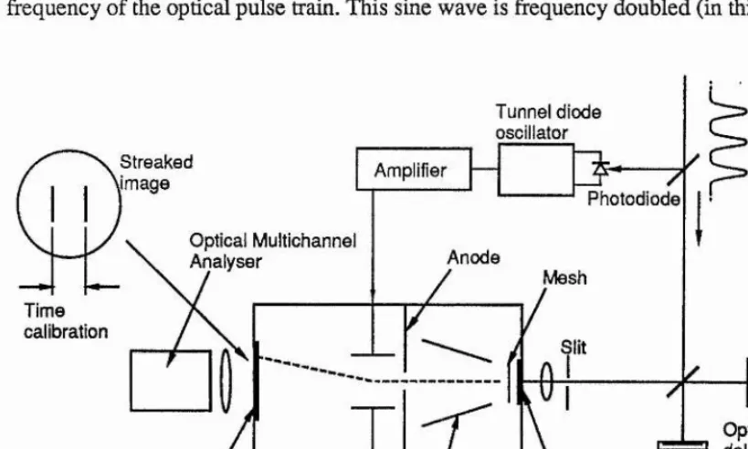
13.1 The Electron - Optical Streak Camera.
a known distance with respect to M2. Each pulse is then directed onto the slit of the streak
camera and imaged onto the photocathode. The number of photoelectrons produced is proportional to the input signal intensity, and so the temporal profile of the pulse is recorded. An anode at high potential accelerates the liberated electrons down the tube where they are deflected by a voltage ramp applied to a pair of deflection plates. The temporal distribution of photoelectrons is converted to a spatial distribution and a 'streaked' image of the pulses appears on the phosphor screen at the rear of the tube. Although the streak camera may be operated in a single shot mode, enabling sub-picosecond resolution [49], it is of great advantage to operate in synchronisation with the mode-locked laser [50], giving a real time display of the pulses. In this case a small fraction of the beam is directed onto a photodiode/tunnel diode oscillator. The tunnel diode is biased so that a pulse incident on the optical diode causes oscillation, and the output is then a sine wave at the exact repetition frequency of the optical pulse train. This sine wave is frequency doubled (in this case to
Tunnel diode
oscillator trainInput pulse Streaked
Jmage Amplifier
Photodiode
Optical Multichannel
Analyser Anode
Mesh Time
calibration
Slit
Optical delay line Deflection
plates Phosphor
screen Photocathode
[image:21.613.90.500.401.647.2]Electron focusing electrodes
Figure 4.
give -164 MHz) to achieve a higher writing speed, and amplified to approximately 10 - 15 W before being applied to the deflection plates. An adjustable electrical delay line ensures that the electrons produced by the light pulses are incident at the deflection plates during the linear section of the deflecting voltage ramp. This ramp is linear to within 5% for approximately one sixth of the period. Streaked images of the pulses are repetitively superimposed on the phosphor screen with picosecond accuracy and the image is directly read using an optical multi-channel analyser (O.M.A). In the work here this was a 500 channel silicon intensified vidicon, having a read out time of ~ 30 ms, giving an image integrated over - 10^ pulses. Both a real time display and plotting a captured image facility were available.
The temporal resolution of the streak camera is limited by the photoelectron transit time dispersion and the technical time resolution. In synchroscan mode, phase jitter between the deflecting voltage ramp and the arrival of the mode-locked pulses also tends to decrease the resolution. Transit time dispersion arises due to an energy spread in the liberated photoelectrons, mainly caused by lattice scattering and pair production within the photocathode. The time dispersion can be expressed in terms of the energy distribution, Ae, and the extraction field at the cathode, E, as [51]:
Operating the photocathode near its long wavelength cutoff, reduces Ae and by inserting a high potential mesh just behind the photocathode, E may be made very large so minimising At. With a cathode-mesh distance of 0.5 mm, extraction fields of « 20 KV/cm are possible enabling subpicosecond transit time dispersions to be obtained. The technical time resolution is dependant on the streak speed and the dynamic spatial resolution (a function of the electron focusing elements). Space charge effects also reduce the resolution as the traveling packet of electrons mutually repel each other.
1.3.2 The Second Harmonic Autocorrelator.
This technique for ultrashort pulse measurement is based upon the process of second harmonic generation (SHG) in a nonlinear crystal [10]. Briefly, the pulse train (of central frequency co) is again incident to an optical delay line, the pulses are divided equally into two and made to overlap in a nonlinear crystal where SHG takes place. A slow, square law detector (photomultiplier tube) detects the light produced at 2co (a filter blocks the residual fundamental light), the level of signal produced being dependent on the temporal overlap of the two sub-pulses. Translating one mirror through the matching point, produces a trace which represents the pulse autocorrelation.
There are essentially two types of SHG autocorrelation corresponding to the two types of phase matching. In type I, the two sub-pulses incident on the crystal are polarised in the same manner whilst for type II, the pulses are orthogonally polarised. Type II phase
matching requires that both pulses be present in the crystal for any SHG to occur and is thus a background free measurement technique. Type I on the other hand, allows second harmonic generation for either pulse, resulting in a pulse on top of a background signal. However, a noncolinear method is also widely used [47], whereby the two pulses are laterally displaced slightly and then combined in the crystal. This also gives a background free detection method. Observation of the peak to background contrast ratio enables a clear indication of the pulse coherence and the Type I colinear method was used throughout this work. A schematic diagram of the SHG autocorrelator is shown in figure 5. Because the detector is relatively slow and responds to the intensity of the signal at 2o), the (normalised) detector output current, la, represents the correlation of the sub-pulses [53]:
Ia(T) = l+2G2(T) + S('i:) (1.4) where G2(t) is the second order correlation function of the intensity of the pulse and is
Oscilloscope or chart recorder
Filter
P.M.T
Variable
delay Nonlinear
[image:24.615.137.429.105.275.2]crystal
Figure 5.
A schematic diagram of the arrangement for second harmonic autocorrelation.
G2(t) =
Jl(t)Kt-x) dt
jP(t) dt
(1.5)
where x is the delay between the two pulses. The S(x) term is a rapidly varying interference term which averages to zero. For a coherent ultrashort pulse of duration Xp (FWHM) we have
Id (0) = 3 and Id (x»Xp) = 1
since 0^(0) = 1 and G^(x»Xp) = 0. Thus the resulting autocorrelation consists of a pulse of (normalised) amplitude 3 on top of a background of unity, as shown in figure 6a. For the case of a free-running laser, with modes oscillating independently, it is still true that Id (0) = 3, since incoherent light is correlated with itself at zero delay. When x>0 or when X is longer than the coherence time of the light, then
where the brackets indicate time averaging. For incoherent light, <I(t)> = l/Vz V <F(t)>, and so (x>0) = 2. This trace is shown in figure 6b. A pulse of incoherent light, or a noise burst, will consist of a narrow coherence spike on top of a broader pedestal, with peak to pedestal to background heights in the ratio 3:2:1 as in figure 6c. Note also that a pulse consisting of N peaks, will give an autocorrelation with 2N-1 peaks. Relating the width of the autocorrelation trace to the FWHM, Xp, of the pulse requires an assumption of the pulse shape since it is seen that the correlation function, G^, is symmetrical and information on the pulse intensity profile is lost The relation between the
3
2
1
0
b.
1
-c.
[image:25.616.115.445.306.656.2]3 “ “
Figure 6.
correlation width, At, and the FWHM of the pulse is
At
(1.7)
where k is a constant depending on the actual shape of the pulse. Table 1 gives values of k for some standard pulse shapes along with the time-bandwidth product, a. Selection of an appropriate pulse shape is some what arbitrary but by measuring the pulse spectrum
simultaneously, the time-bandwidth product for each shape may be deduced and the one
closest to the particular a selected. A more precise method is to use higher order correlation functions which enable the direct determination of pulse shape.
Table 1.
Pulse Shape Intensity profile k a
Square 1 lti<Tp/2
0 ltl>tp/2 1 0.886 Gaussian
/ 41n2 t^ >
V2
0.441 exp- ...—-....__1
V
V HyperbolicSech^ sech^ (1.761/Xp) 1.55 0.315
List of autocorrelation correction factors and time-bandwidth products for some typical pulse shapes, tp is the pulse FWHM.
Unfortunately however, these require even higher powers and signal detection becomes a major problem.
Ihterferoroetric autocorrelatioii&
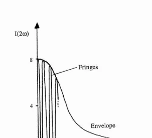
In this case the scanning mirror is scanned slowly or, equivalently, the response time of the square law detector is increased. The interference term in equation (1.4) is then resolvable and the autocorrelation trace shows the fringes associated with the interference of the two pulses overlapping in the crystal. A typical interferometric autocorrelation trace is shown in figure 7. The peak to background contrast ratio increases to 8:1, while at the centre of the pulse the minimum signal level is zero. The autocorrelation is now self calibrating since the separation between the interference peaks is equal to one wavelength.
I
-1
However, it is somewhat more difficult to infer a pulse duration from this type of autocorrelation since the shape of the envelope is extremely sensitive to frequency chirp on the pulse. By fitting a computer generated envelope to the interferometric autocorrelation, the discrepancy from a standard pulse shape may be determined and an indication of the amount of frequency chirp obtained. It has been shown [54], that a linear chirp such as that produced by dispersion alone, leads to rising wings in the autocorrelation, while nonlinear chirp (from say SPM) causes excessive fringing in the wings.
1(2(0)
Fringes
E n v elo p e
[image:27.614.156.459.278.553.2]0 X
Figure 7.
Appearance of a typical interferometric autocorrelation.
The temporal resolution of the SHG autocorrelation method is determined by the
bandwidth over which phase matching may occur in the crystal - the phase matching
but also the resolution is improved, since the interaction length or the effective crystal thickness, is reduced. At 1.5 jim a 2mm crystal was seen to have a resolution of approximately 200 fs. A 2mm thick piece of LiNbOg was used for most pulse width
measurements down to approximately 0.5 ps and for pulse durations less than this, a 100 jim piece of KDP was used. It has also been shown that pulse to pulse duration fluctuations affect the measured autocorrelation width. Since the SHG efficiency is increased for higher peak powers (shorter pulses) the autocorrelation tends to weight shorter pulses more favourably and therefore probably gives a pulse width measurement less than the true average [57].
For autocorrelations at 1.5 pm, the PM tube, nonlinear crystal and focusing lens were all enclosed within a light tight box and optical access was through an AR coated silicon filter. This had a transmission cut on at =1.32 pm allowing only fundamental 1.5 pm light through, enabling autocorrelations to be taken in normal room light. By mounting one
mirror (actually comer cubes were used so as to enable a sideways displacement of both
beams) on a motor driven translation stage, a hard copy trace of the autocorrelation could
be taken over a period of » 30s. Also one mirror was mounted on a loud speaker and vibrated at about 25 Hz, enabling a real time monitor of the pulse duration to be displayed on a simple oscilloscope [58] greatly facilitating optimisation of the mode-locked laser.
It is worth pointing out that the straight forward linear autocorrelation (i.e no second harmonic crystal) records no more information than the spectrum of the pulse, it is simply presented in a different form than usually encountered. If the first order correlation were to
be measured, information on the coherence length of the pulse is obtained which is only related to the actual pulse duration in the bandwidth limited case.
1.4 A Brief Review of the Guiding Properties of Optical Fibres.
telecommunications networks. Much of the work here has involved the propagation of pulses in single-mode fibres and while chapter 3 is devoted to a study of nonlinear pulse propagation, a brief review of the general guiding properties of optical fibres is appropriate here.
An optical fibre is a cylinder made from transparent dielectric materials, usually based on fused silica (SiOi). A central region, the core, is surrounded by a cladding region of lower refractive index and the whole structure is normally coated in a protective jacket. The optical characteristics of a fibre are determined by its refractive index profile which is usually circularly symmetric, depending only on the radial coordinate. Many types of fibre with different refractive index profiles exist [59], that of a 'step index' circular optical fibre is given by
n(r) = ni r < a
Ü
. 2 r > awhere a is the core radius. As in figure 8 the basic guiding principle is that light incident to the cladding layer from the core, at an angle greater than the critical angle, will
be reflected. Successive reflections guide the radiation down the fibre.
'clad '
Figure 8.
(a) Refractive index profile of a step index fibre, (b) Guiding nature of a circular optical fibre.
For such a fibre the maximum acceptance angle, 0 ^», to the fibre axis within which the
no sin = ni(l - sin^QJi/^ = (n^^ -
n
2^y^
(1.8)where no is the index of the medium surrounding the fibre (usually air), n, and U2 are
core and cladding refractive indices respectively. The quantity (n^^ -
Ü
2^y^
is known as thenumerical aperture of the fibre. If the fibre is bent to severely, then radiation may leak from
the fibre and losses are incurred. These are known as bending losses.
The ray picture of light propagating in a fibre is somewhat simplistic and the full solution is obtained by solving Maxwells equations in the core and cladding regions. Since the fibre is of circular geometry, the equations are written in spherical coordinates and the
boundary conditions of (i) matching fields at the interface and (ii) a decaying (non- radiative) field in the cladding, are applied. The solutions are derived in many standard texts [59,60] and are in the form of Bessel functions. For the guided mode, there exists a discrete set of solutions and the mode propagation constant may not take on any arbitrary value. TE and TM mode solutions exist as well as hybrid modes, labeled HE and EH, which have longitudinal electric and magnetic field components. In terms of a ray analogy, the TE and TM modes correspond to meridional rays and the hybrid modes to skew rays. The finite number of discrete modes leads to a finite number of possible propagation constants within the guide. These fall within the range
n2 k < I Pg I < ni k
where p, is the guided mode propagation constant and k (=27tA) the free space propagation constant. A constant A is known as the average core/cladding index difference and defined as
A
.
(1.9)It is usually the case that A « 1 and a fibre with this property is known as a weakly guiding fibre [61]. In this case it can be shown that the guided modes are very nearly linearly polarised and are designated LP modes [61].
It also turns out that a parameter known as the fibre 'V number [59-61], determines
V = 27[Aa(ni2_n22y/2
= kani(2A)w (1.10)
for the case of A « l. The number of modes is given approximately by N = W 2. As V becomes close to the cutoff value for a particular mode, progressively more radiation is carried in the cladding region. When V< 2.405 only the single LPoi mode may exist in the fibre and all others are radiation modes. The fibre is then said to be single-mode. (There are actually two modes possible with orthogonal polarisations, the term single-mode refers to the case of a single input polarisation). It is possible therefore to construct a fibre to be single-mode at a given wavelength by choosing appropriate values of A and core radius a.
Polarisation maintaining fibres.
Single-mode fibres do not normally preserve the polarisation state of the input signal. An ideal fibre can support two independent modes of arbitrarily orthogonal polarisations,
both as fundamental HE^ modes. These modes would have the same phase velocity and the polarisation would be a linear superposition of these two polarisation eigenmodes. In a real fibre however, imperfections such as stresses and a noncircular core, lift the degeneracy of the two modes causing a difference in the effective refractive index for each
mode and they propagate with different phase velocities. This index difference is known as the fibre birefringence. Normal single-mode fibres have a low birefringence which is sensitive to external influences such as bending, twisting, temperature, applied pressure and stray electric and magnetic fields. These effects cause scattering between the two polarisation states and the output polarisation becomes pseudorandom and unpredictable. Some control over the output polarisation may be achieved by bending or stressing the fibre [62], and provided the surrounding conditions are constant, the polarisation will then remain steady. In fact low biréfringent fibres are useful in sensing applications where a change m external conditions causes a measurable change in the polarisation state [63]. In
achieved by geometrical or stress induced methods. A fibre with a highly elliptical core and large index difference between the core and cladding, enables high internal birefringence and polarisation maintaining properties to be obtained but the core then needs to of small
dimensions in order to preserve the single-mode nature [64]. Other methods of obtaining a high birefringence involve surrounding the core with an elliptical or nonsymmetrical region in the cladding. More detailed reviews of high biréfringent fibres may be found in references [65,66].
Fibre dispersion.
Dispersion in a single-mode fibre is composed of two effects, material and waveguide dispersion. The first of these simply arises from the well known variation in refractive index with wavelength in a dielectric material. The second derivative of this with respect to wavelength, d^n/dX^, gives rise to group velocity dispersion (GVD), causing a spreading or
broadening of an optical pulse propagating along a fibre. As will be described in chapter 5, the GVD of fused silica passes through zero at = 1.3 pm, becoming anomalous for wavelengths greater than this, i.e the group velocity decreases with increasing wavelength [67]. Waveguide dispersion also causes GVD but is due to the variation of the guided
mode velocity with the fibre V parameter [59]. If the mode is not close to cutoff then
material dispersion usually dominates. For the case of a small core however (such as that encountered in elliptical core fibres), waveguide dispersion can become important and significantly alter the dispersion characteristics of the fibre [68].
1.5 Conclusions.
In this introductory chapter a brief description of the process of mode-locking has been presented along with two techniques for the measurement of ultrashort pulses which were extensively used in the work for this thesis. An introduction to the guiding properties of optical fibres has also been given.
self-phase modulation and stimulated Raman scattering and their applications to optical pulse compression and fibre Raman oscillators. The direct generation of tunable NIR optical pulses around the important wavelength region of 1,5 |im using colour centre lasers, is described in chapter 4 and the nonlinear propagation of such pulses in optical fibres, leading to the phenomena of optical solitons is presented in chapter 5. By combining a length of optical fibre into the feedback loop of a KCliTl colour centre laser, it is shown in
both chapters 5 and 6, that subpicosecond NIR pulses may be produced, enabling this
References.
1. M DiDomenico; J Appl. Phys. 35, 2870 (1964)
2. LE Hargrove, R L Fork, M A Pollack; Appl. Phys. Lett. 5, 4 (1964)
3. A Yariv; J Appl. Phys. 36, 388 (1965)
4. H Statz, C L Tang; Quant. Electronics IE, P Grivet, N Bloembergen Eds. Columbia University Press p.469 (1964)
5. E O Ammann, B J McMurtry, M K Oshman; IEEE J Quant. Electron. QE-1,263 (1965)
6. M DiDomenico, H M Marcos, J E Geusic, R E Smith; Appl. Phys. Lett. 8,180 (1966)
7. S E Harris; Proc. IEEE 54, 1401 (1966)
8. H W Mocker, R J Collins; Appl. Phys. Lett. 7, 270 (1965)
9. R L Fork, C V Shank, R Yen, C A Hirlimann; IEEE J Quant. Electron. QE-19,500 (1983)
10. J A Armstrong; Appl. Phys. Lett. 10,16 (1967) 11. H P Webber; J Appl. Phys. 38, 2231 (1967)
12. S Y Wang, D M Bloom, D M Collins; Appl. Phys. Lett. 42, 190 (1983)
13. W Sibbett; SPIE 348, Conference on High Speed Photography, San Diego (1982) 14. C V Shank, R L Fork, R F Leheny, J Shah; Phys. Rev. Lett. 42, 112 (1977)
15. L Reekie, I Ruddock, R Illingworth; in 'Picosecond Chemistry and Biology’T Doust, M West Eds. Sience Reviews Limited (1983)
16. D S Chemla, D A B Miller; J Opt. Soc. Am. B 2 ,1155 (1985)
17. R J Manning, D W Crust, D W Craig, A Miller, K Woodbridges; J Mod. Optics 35,
541 (1988)
18. D H Auston, M C Nuss; IEEE J Quant. Electron. QE-24,184 (1988) also in same issue; K J Weigarten, M J W Rodwell, D M Bloom; p. 198
19. P Kaiser, W T Anderson; J Lightwave Tech. LT-4,1157 (1986)
22. C V Shank, R L Fork, F Beisser; Laser Focus p.59 June 1983
23. M D Dawson, T F Boggess, A L Smirl; Opt. Lett. 12, 590 (1987)
24. P Beaud, B Zysset, A P Schwarzenbach, H P Webber; Opt. Lett. 11,24 (1986) 25. H Lobentanzer, H J Polland; OPt. Comm. 62, 35 (1987)
26. C R Pollack, J F Pinto, E Georgiou; Appl. Phys. B 48,287 (1989) 27. N Langford, K Smith, W Sibbett; Opt. Lett. 12, 817 (1987)
28. N Langford, K Smith, W Sibbett; Opt. Lett. 12, 903 (1987) 29. F M Mitschke, L F Mollenauer, Opt. Lett. 12,407 (1987) 30. A E Siegman, D J Kuizenga; Opto-Electronics 6,43 (1974) 31. D J Bradley, G C H New; Proc. IEEE 62, 313 (1974) 32. P W Smith; Proc. IEEE 58,1342 (1970)
33. D J Kuizenga, A E Siegman; IEEE J Quant. Electron. QE-6,694 (1970) 34. G H C New, L A Zenteno; Opt. Comm. 48, 149 (1983)
35. A J De Maria; J Appl. Phys. 34, 2984 (1963)
36. C P Ausschnitt, R K Jain, J P Heritage; IEEE J Quant. Electron. QE-15,912 (1979) 37. M D Dawson, D Maxson, T F Boggess, A L Smirl; Opt. Lett. 13, 126 (1988) 38. U Stamm, F Weidner, Appl. Phys. B 48, 149 (1989)
39. D J Kuizenga, A E Siegman; J Quant. Electron. QE-6,709 (1970) 40. E P Ippen, C V Shank, A Dienes; Appl. Phys. Lett. 21, 348 (1972) 41. H A Haus; J Appl. Phys. 46, 3049 (1975)
42. J A Valdmanis, R L Fork, J P Gordon; Opt. Lett, 10,131 (1985) 43. A Finch, G Chen, W Sleat, W Sibbett; J Mod. Optics 35, 345 (1988)
44. D J Parker, P J Say, A M Hanson, W Sibbett; Electron. Lett. 23,527 (1987) 45. A Finch, W E Sleat, W Sibbett; Rev. Sci. Instrum. To be published (1989) 46. R L Fork, C H Brito Cruz, P C Becker, C V Shank; Opt. Lett. 12, 483 (1987) 47. E P Ippen, C V Shank; Chapter 2 in 'Ultrashort Light Pulses' Ed. S L Shapiro,
Springer Verlag (1977)
49b A Finch, Y Lui, H Niu, W Sibbett, W E Sleat, D R Walker, H Yang, R Zang; Ultrafast Phenomena VI Springer series in chemical physics 4 8 ,159 (1988)
50. M C Adams, W Sibbett, D J Bradley; Advances in Electronics and Electron Physics
52, 265 (1979)
51. W Sibbett; PhD Thesis, Queens University of Belfast (1973) 52. J P Willson, W Sibbett, W E Sleat; Opt. Comm. 42, 208 (1982) 53. A Yariv; 'Optical Electronics' chapter 6 Holt & Saunders 3"*^ ed. (1985)
54. J M Diels, J J Fontaine, IC McMichael, F Simoni; Appl. Opt. 24, 1270 (1985) 55. AM Weiner, IEEE J Quant. Electron. QE-19,1276 (1983)
56. J Comly, E Garmire; Appl. Phys. Lett. 12,7 (1968) 57. E W Van Stryland; Opt. Comm. 31,93 (1979) 58. R L Fork, F A Beisser; Appl. Opt. 17, 3534 (1978)
59. 'Optical Fibre Telecommunications' S E Miller, A G Chynoweth Eds. Academic (1979)
60. A H Cherin, 'An Introduction to Optical Fibres' McGraw-Hill (1983) 61. D Gloge; Appl. Opt. 10, 2252 (1971)
62. H C Lefevre; Electron. Lett. 16,778 (1980) 63. See papers in J Lightwave Tech. LT-5 (1987)
64. R B Dyott, J R Cozens, D G Morris; Electron. Lett. 15, 380 (1979)
65. M P Vamham, D N Payne, A J Barlow, R D Birch; IEEE J Lightwave Tech. LT-1,
332 (1983)
66. J Noda, K Okamoto, Y Sasaki; IEEE J Lightwave Tech. LT-4,1071 (1986) 67. D N Payne, W A Gambling; Electron. Lett. 1 1 ,178 (1975)
Chapter 2.
The Acousto-Optically Mode-Locked Nd:YAG Laser.
2.1 Introduction.
The NdrYAG laser was first developed in 1964 [1] and is now well established as a pump source for dye lasers [2,3] and colour centre lasers [4]. Both the fundamental emission (1.064 pm) and the second harmonic (532 nm) are extensively used for optical pumping and other applications such as Raman generation and pulse propagation studies in optical fibres [5-7]. Mode-locking of this laser was first demonstrated by DiDomenico et al [8], producing pulses of = 80 ps duration with intracavity acousto-optic (AO) loss
modulation. Later Ostemik and Foster [9] obtained 30 ps pulses using an electro-optic phase modulator.
Due to homogeneous line broadening within the gain medium, NdrYAG lasers are almost exclusively actively mode-locked. This method of mode-locking does not generally produce pulses as short as passively mode-locked systems and it is also more difficult to control the stability of the output pulse train. While passively mode-locked Y AG lasers operating in a pulsed mode have generated pulses as short as 28 ps [10], it is generally
more convenient to have a continuous train of pulses as provided by AO mode-locking. In
common with other solid state lasers, the CW pumped NdrYAG laser is susceptible to
relaxation oscillations [11,12] causing output fluctuations in both pulse width and amplitude. Careful design of the laser resonator and the use of active feedback systems for
2.2 The Spectra Physics Series 3000 Laser System.
Neodymium doped Yttrium Aluminum Garnet is the gain medium of the so called 'YAG' laser and possesses properties which are highly favourable for laser operation. About 1% of Y^+ ions are substituted by Nd^+ ions and the energy level of these ions in YAG are shown in figure 1. The medium constitutes a four level system and together with a narrow fluorescent line width, results in a low threshold for laser operation. Although several laser transitions exist, giving operation at 940nm and 1.36 pm, the well known 1.064 pm line is the strongest. This transition occurs from the upper component of the level to the level which is 2111 cm-^ above the ground state. Hence the population of this level at room temperature is only a factor of exp(AE/KT) ~ exp(-lO) of the ground state density. The fast relaxation of the nonradiative transition Hi 1/2 —>
%a
and the fact that thei %
Î
2 0
-1 0
-0-^
4p.3/2
4|11/2
Pump bands
(5 round Level
■11502 cm'"*
Laser transition (1.064 pm)
[image:38.614.133.451.355.663.2]•2111
Figure 1.
lower level is not thermally populated, both ensure that the threshold condition is easily reached. A number of broad pump bands exist, those at 810 nm and 750 nm being the strongest. Thus the Nd:YAG medium is well suited to optical pumping by a high pressure Krypton arc lamp [13]. The fluorescent efficiency of the upper laser level is ~ 99.5% which means that almost all the ions excited from the ground state end up in the upper laser level. The spontaneous fluorescent lifetime of this level (which includes all possible
decays) is ~ 230 ps. This value is long indeed compared to that for ion lasers and dye lasers. Some physical and optical properties are summarised in table 1.
Table 1.
Chemical formula NdiYsAlgOiz
Nd atoms / cm^ 1.38X 10²⁰
Thermal conductivity 0.13Wcm-iK-i
Line width 4.5 Â (120 GHz)
main lasing transition 1.064 fim
o 8.8x 10⁻¹⁹ cm2
X 230 jis
n 1.82 (at 1.06 |Ltm)
Some physical and optical properties of Nd:YAG. a stimulated emission cross section; t
spontaneous fluorescent Lifetime; n refractive index. (After reference [12])
The laser used in these experiments was a Spectra Physics series 3000 NdrYAG. The active medium was in the form of a 4 mm diameter cylinder, with a length of approximately 80 mm. This was located at one focus of a gold coated elliptical reflector chamber and pumped with a high pressure Krypton arc lamp, located at the other focus. The lamp was
typically run at a current of 17 A but this needed to be increased as the lamp aged. Lamps
were changed after approximately every 400 hours of use. Two pyrex flow tubes placed
over the lamp and rod prevented UV tight being incident on the rod which would otherwise cause a decrease in the output power due to the formation of colour centres. The total power dissipated in the lamp was approximately 2 - 3 kW, causing considerable heating of
A major problem in the design of high power Nd:YAG lasers occurs due to the heating of the rod by optical pumping. The low thermal conductivity of Nd:YAG leads to a radial temperature gradient being set up, which causes the rod to behave as a thick lens for light propagating along its axis. The effective focal length depends on the output power from the lamp and therefore on the lamp current, higher currents giving shorter focal lengths. The laser resonator was designed to stay within the stability condition over the widest possible range of currents. If the current is too large, the cavity becomes unstable due to the strong focusing of the rod. In some lasers a concave - convex mirror arrangement is implemented, the focusing effect of the rod being used to compensate for the diverging effect of the convex mirror [14]. However, in the Spectra laser two concave mirrors of radius 60 cm were used, separated by approximately 1.8 m. The Nd:YAG rod was positioned in the centre, giving an overall optical path length of « 1.86m. The beam diameter changes within the cavity, being largest at the rod allowing maximum extraction of energy from the gain
medium - see figure 2.
YAG rod Mirror
r = 60
- 2 mm
0
Figure 2.
Typical beam profile within the Nd:YAG laser cavity.
The output mirror had a reflectivity of 85% and the laser gave typically 7 to 8 W time averaged output power (mode-locked) in a vertically polarised TEMqobeam,
2.2.1 The Acousto-Optic Mode-Locker.
Mode-locking of the laser was achieved by using an intracavity acousto-optic loss
the rear of the laser, such that reflection losses from the prism were minimised. Figure 3 shows a schematic diagram of the device and the optical beam is incident normally to the ultrasonic standing wave (known as the Raman-Nath regime). The mode-locker had 20 to 30 resonances separated by 400 kHz and centred on 41 MHz. The separation of these resonances is obtained from the usual formula, c/2L, where here L is the width of the prism and c is the velocity of sound in the crystal. When the frequency of an r.f driver signal matches one of the resonances, the modulator appears as a 50 Q load and maximum power transfer to the crystal takes place. This results in maximum diffraction efficiency and
optimum mode-locked performance.
Brewster
Laser output
angle
Mode-locker crystal
Transducer
Figure 3.
A schematic diagram of the AO mode-locker.
However, the frequency of the resonance is extremely temperature dependent and so any fluctuations of the modulator temperature will cause changes in the diffraction efficiency and fluctuations in the mode-locked output An oven around the modulator keeps its temperature constant and held a few degrees above ambient, prevents room temperature fluctuations disrupting the mode-locking. Heating of the mode-locker crystal still occurs from the laser beam itself and the applied r.f signal, which was typically 1 - 2 W. As the crystal is heated, the resonance frequency of the crystal rises and as it does so the coupling of r.f power into the crystal falls, allowing the crystal to cool. The resonance frequency then falls again, until it coincides with the driver frequency. Many AO mode-lockers operate in this metastable condition, with the diffraction efficiency being less than
driver frequency exceeds that of the resonance, the coupling efficiency is again reduced and the crystal will cool further, increasing the difference between the driver and resonant frequencies. This effect is known as thermal runaway and mode-locking will be lost. To over come this, the Spectra Physics mode-locker used an active feedback loop controlling the r.f power applied and hence the temperature of the crystal. The system was developed
by Klann et al [15] and is shown diagrammatically in figure 4.
Directional coupler Amplifier
To
transducer
Phase delay network Power splitter R.F Driver
Phase detector (Doubly balanced mixer)
Voltage controlled attenuator
Figure 4.
Schematic diagram of the active feedback loop employed with the mode-locker.
driver frequency and there is no danger of thermal runaway. Also higher r.f powers may be used enabling greater diffraction efficiencies.
The mode-locker electronics provided a step wise variation of the drive frequency as well as a fine frequency control, giving ~ ± 300 Hz adjustment. Also the modulator position could be varied via a screw thread, enabling the cavity length to be matched to that coixesponding to twice the acoustic frequency. Once the laser was mode-locked, occasional adjustments of the frequency were required for optimum stability but it was very seldom
that mode-locked operation was lost.
Another useful advantage obtained with this type of active stabilisation, is that is possible to increase the modulation applied to the laser field. A higher modulation depth in the AO modulator essentially means that the mode-locker appears transparent to the optical field for a shorter time period, thus giving rise to the production of shorter pulses. This was achieved in the following way. Once the laser had been initially mode-locked onto a crystal resonance, the r.f drive frequency was gradually stepped up. As the feedback loop
detected a frequency mismatch, the servo system increased the r.f power applied to the
modulator thereby also pushing up the crystal resonance. Hence a higher power is applied to the transducer increasing the acoustic modulation and by following the increased frequency with a decrease in cavity length, improved mode-locked operation is obtained.
23 Laser Performance and characterisation.
The laser is specified to produce time average powers > 7 W with a mode-locked pulse duration of 120ps. For the majority of the work reported in this thesis, the laser did meet these specifications although over the last few months a gradual decline in output power occurred. A schematic diagram of the experimental arrangement for the laser characterisation is shown in figure 5. The photodiode was an AEG Telefunken BPW 28 which provided a trigger for the streak camera system (see chapter 1) and also enabled
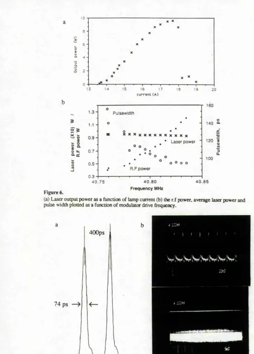
Initially the output power as a function of lamp current was recorded and the results are shown in figure 6a. The cavity clearly begins to become unstable at a current of ~ 17.6 A. Note that the absolute values of current indicated here only apply to this particular lamp, alignment etc., and will vary with different lamps and time. It was predicted that increasing the mode-locker drive frequency and thereby the modulation depth, should enable the production of shorter pulses. This was evaluated experimentally by gradually increasing
Photodiode
---1 M
O.M.A. Frequency Counter
Amplifier Tunneldiode
oscillator
Oscilloscope Modulator
electronics
Spectrum analyser
Streak camera Nd:YAG
M
Figure 5.The experimental arrangement for a laser characterisation.
the r.f frequency and optimising for the best pulses at each step by shortening the cavity length. The plots in figure 6b show the increase in applied r.f power and corresponding decrease in pulse duration as the frequency was incremented. The average laser power remained approximately constant. In figure 7 the recorded streak camera traces of the shortest pulses obtained are shown, along with a photograph of a typical pulse train.
o 2
16 17
c u r r e nt (A)
1.3 H
* 1.,
2 3
ÎS « 0.9
-o 0.7
-a. oc
0.5-40.75
Pulsewidih
x x x x x x x x x x x x x
• Laser power
R.F power
o o
o o o o
160
140
û-■o
120 ‘i
[image:45.615.20.541.14.741.2]— 3 CL 100 40.80 Frequency MHz 40.85 Figure 6.
(a) Laser output power as a function of lamp current (b) the r.f power, average laser power and pulse width plotted as a function of modulattw drive frequency.
400ps
74 ps —>
' I I I I ' ' ’
,
V Ii'v 'ÏV iNt»* ÏV ijv ii'v
IICrS
Figure 7.
sufficient intensity to constitute a second pulse. However, by correct alignment of the ü cavity short pulses could be produced with only slight pulse asymmetry. It was noted that
the laser pulse duration and stability were very sensitive to the mode-locker frequency and so an investigation into frequency detuning effects was conducted. It was found easier and
more reliable to alter the modulator frequency, leaving the cavity length unchanged. This was because fine frequency adjustments could be made without affecting the resonator alignment as might easily be the case by trying to adjust the resonator on the length control.
In any case, the two adjustments have the same effect, decreasing the frequency would be i
the same as decreasing the cavity length.
Pulse amplitude fluctuations for the optimally mode-locked Nd:YAG were found to have two major components. (Optimal mode-locking is taken here to mean minimum pulse
duration). The first component was a regular ripple ( ~ 3% peak-to-peak) on a millisecond timescale attributed to the Krypton arc lamp power supply. The second was manifest as a pair of sidebands separated from the central ~ 82 MHz spectral peak by ~ 60 KHz on the spectmm analyser, and also as a
4%
ripple with period 15 |is on the oscilloscope. This is seen in figure 8a. The second component may be attributed to relaxation oscillations in the gain medium [11,16]. Relaxation oscillations and spiking are common in lasers where the recovery time of the excited state population inversion is substantially longer than the cavity decay time. In other words, if the gain medium has a long upper state lifetime compared to the cavity decay time. Solid state lasers are particularly prone to this type of oscillation and is a major cause of instability. The relaxation period is a characteristic of the cavity and gainmedium, resulting from an interplay between the optical field and population inversion. An increasing optical field intensity depletes the inversion, lowering the optical gain available until at some point the optical field begins to decrease. This means that less stimulated emission occurs allowing the inversion to build up again and the cycle is repeated. Generally the oscillations result from some perturbation of the laser and exponentially decay away. However if some driving force is present, the oscillations may be sustained
35
H — 400 ps H |<—400ps
[image:47.619.8.535.20.713.2]79 ps 119 ps
Figure 8.
Synchroscan streak camera intensity profiles of (a) short puises (f = 40.800272 MHz) and (b) puises corresponding to minimum 60 kHz modulation (Af » -181 Hz). The photographs show puise amplitude fluctuations for each case. (200 mV/div; 10 |xs/div).
150
CO
a c
o
^
100 «3 OL50
- 1.0 -0.5 0 + 0.5
Frequency detuning , kHz
Figure 9.
The dependence of mode-locked pulse duration on frequency detuning from the optimum modulator frequency (f = 40.800272 MHz). The shaded area indicates the region of minimum sideband intensity.
detunings, greater pulse durations with an increased presence of the 60 kHz modulation were observed. However even at the largest negative detuning (~ -1 kHz) shown in figure 9, the 60 kHz modulation depth (or sideband intensity) did not approach the magnitude experienced at only 500 Hz positive detuning where similar pulse durations were recorded. A positive frequency detuning of only 50 Hz caused a marked increase in the amplitude
modulations and instabilities due to relaxation oscillations.
stability in terms of amplitude fluctuations, Q-switched oscillation period and envelope duration was very poor. On the negative detuning side the stability of the Q-switched output was excellent with peak-to-peak amplitude fluctuations as low as 5% on a
millisecond timescale. Figure 10 shows the onset of the Q-switched operation. During self Q-switching operation the spectrum analyser revealed a series of stable sidebands (typically 5-10 pairs) separated by 50 - 100 kHz. Time average output powers of = 7.5 W were typical during this behaviour. Figure 11 shows how both the oscillation period and the envelope duration varied as a function of frequency detuning. It can be seen that as the frequency was decreased, the oscillation period decreased and the envelope broadened. In addition it was noted that the magnitude of the Q-switched envelope increased for smaller
frequency detunings, in accordance with the observation that the average power remained essentially constant. This overall behaviour was also
Î ‘ A - I
jË i
[image:49.614.14.539.256.781.2]m
Figure 10.
20_
-7
-6
JZ
-3.5
[image:50.620.105.443.25.415.2]-2.5 -3.0
Figure 11. Frequency detuning . kHz
Plot of Q-switched oscillation period (crosses) and envelope width (dots) as a function of frequency detuning.
observed for positive frequency detuning. The Q-switched envelope was composed of
many mode-locked pulses and in order to obtain an estimate of the Q-switched mode-
|< - 600 ps
2 3 7 p s
Figure 12.
Synchroscan streak camera intensity profiles of the Q-switched mode-locked pulses. (Af » -2.1 kHz)
Investigation of the background radiation between the Q-switched envelopes, using the 7834 oscilloscope, revealed mode-locked pulses whose energy content was about 10^ smaller than those at the peak of the envelope, however the picosecond nature of the pulses did not decay between the Q-switched spikes.
2.4 Conclusions.
KC1:T1 colour centre laser. In particular, the operation of the ’Soliton’ laser (chapters 5,6) was found to be dependant upon a stable pump source. The drawback of a slight increase in pump pulse duration, was more than offset by greater laser stability.
For the work in the following chapter, an AO modulator as described above was used. However, for the optical pumping of the KC1:T1 colour centre laser described in chapter 4, a new mode-locker was used which operated in the Bragg regime and was situated just
before the output coupler. The laser exhibited a similar behaviour with this new mode- locker and was usually operated in the region of minimum noise. Under these conditions the pulse duration was typically 100 ps with ~ 3% peak-to-peak amplitude modulations due to the Krypton arc lamp power supply.
References.
1. JE Geusic, H M Marcos, L G Van Hitert; Appl. Phys. Lett. 4, 182 (1964) 2. A Seilmeier, W Kaiser, B Sens, K H Drexhage; Opt. Lett. 8, 205 (1983) 3. P Beaud, B Zysset, A P Schwartzenbach, H P Weber; Opt. Lett. 11, 24 (1986) 4. L F MoUenauer, N D Vieira, L Szeto; Opt. Lett. 7,414 (1982)
5. B P Nelson, D Cotter, K J Blow, N J Doran; Opt. Comm. 48, 292 (1983) 6. A S L Gomes, W Sibbett, J R Taylor, Appl. Phys. B 39, 43 (1986)
7. AS Gouveia-Neto, M E Faldon, A S B Sombra, P G J Wigley, J R Taylor; Opt. Lett.
13, 901 (1988)
8. M DiDomenico, J E Geusic, H M Marcos, R G Smith; Appl. Phys. Lett. 8, 180 (1966)
9. L M Ostemik, J D Foster; J Appl. Phys. 39,4163 (1968) 10. A R Globes, M J Brienza; Appl. Phys. Lett. 14, 287 (1969) 11. W Koechner; IEEE J Quant. Electron. QE-8, 656 (1972)
12. W Koechner; ’Solid State Laser Engineering' Springer Verlag (1988) 13. T B Read; Appl. Phys. Lett. 9, 342 (1966)
14. R B Chesler, D Maydan; J Appl. Phys. 43, 2254 (1972)
15. H Klann, J Kuhl, D Von der Linde; Opt. Comm. 38,390 (1981) 16. A Yariv; 'Optical Electronics' 3^^^ ed. Holt and Saunders (1985) 17. A Siegman; 'Lasers' University Science Books (1986)
18. H J Eichler, Opt. Comm. 56, 351 (1986)
19. M J W Rodwell, K J Weingarten, D M Bloom; Opt. Lett. 11, 638 (1986)
Chapter 3.
Nonlinear Pulse Propagation in Optical Fibres.
3.1 Introduction.
Since the development of the laser in 1960, a revolution has taken place in the field of nonlinear optics. Our knowledge and understanding of the behaviour of matter under the influence of intense optical fields has been dramatically increased and a whole range of new phenomena have been discovered [1,2]. The availability of low loss, single-mode optical fibres has recently opened up a new era in nonlinear optics, due mainly to the following reasons: (1) the small core sizes (typically ~ 2-8 jim in diameter) enable high power
densities to be achieved with relatively low input powers; (2) these high power densities can be maintained over long distances due to the guiding nature of optical fibres and so greatly increased interaction lengths are obtained compared to bulk materials; and (3) the transverse profile of the beam is well characterised and virtually all of the beam experiences
the same nonlinearity [32], These factors can considerably lower the threshold powers required for the nonlinear processes. While it is considered that nonlinear effects in optical fibres will be the main optical power limitation to an optical communications network, some of these same effects have potentially useful applications as optical amplifiers and oscillators and the nonlinear propagation of pulses in fibres has been extensively studied over the last few years. The main nonlinear processes in optical fibres are: stimulated Brillouin scattering (SBS), stimulated Raman scattering (SRS), the optical Kerr effect, self-phase modulation (SPM), four-photon mixing, nonlinear absorption and most recently second harmonic generation.
pressure (acoustic) wave due to électrostriction, which then scatters some of the pump creating a Stokes wave. The frequency shift of the Stokes from the pump light depends on the scattering angle and is a maximum for 180° and zero for 0°. Thus in optical fibres SBS only creates a backward traveling wave. The Brillouin gain coefficient, Gb (~ 4.3x10* ^^m/W) is dependent upon the ratio of the Brillouin linewidth, Aog, to the pump linewidth, At)p. For the case were A\)p « ADg, the gain coefficient is independent of AOp, but for At)p > ADb it is proportional to AOg/ADp [4]. In fused silica 38 MHz at
X~
1.0 pm and it varies as X*^. The threshold (or critical power, since there is no actual 'threshold' value) for SBS is [4]= (3.1)
where A is the effective core area and L is the effective fibre length which is different from the actual length, 1, due to fibre loss (see section 3.2.1). The factor of two is included for fibres that do not preserve the input polarisation. Typically, in our experiments L= 1 ~ 200 m (since the fibre loss is small -0.9 dB/km), A - 4x 10*^^ and using a CW mode- locked Nd:YAG laser,