Size and Shape Analysis of Error-Prone Shape Data
Jiejun DU, Ian L. DRYDEN, and Xianzheng HUANG
We consider the problem of comparing sizes and shapes of objects when landmark data are prone to measurement error. We show that naive implementation of ordinary Procrustes analysis that ignores measurement error can compromise inference. To account for measurement error, we propose the conditional score method for matching configurations, which guarantees consistent inference under mild model assumptions. The effects of measurement error on inference from naive Procrustes analysis and the performance of the proposed method are illustrated via simulation and application in three real data examples. Supplementary materials for this article are available online. KEY WORDS: Complex normal; Configuration; Landmark; Ordinary Procrustes analysis; Quaternion.
1. INTRODUCTION
Data capturing the size and shape of an object are of great interest in many branches of science. For instance, facial recog-nition as a routine task in forensics relies on shape data of faces; chemists study shapes of molecules to understand and manipulate chemical properties; and study on shapes of com-plex organisms is an important part of research in biology and medicine. One approach that has a long history for character-izing sizes and shapes entails defining landmarks on an object, the collection of which is referred to as the configuration of the object (Kendall1984; Bookstein1991; Dryden and Mardia
1998). Then the shape data for this object consist of the geo-metric information of these landmarks in the configuration after removing location, rotation, and (possibly) scale. This way of measuring shape data has been adopted in biology, for example, among many other fields where applied scientists understand well the choice and interpretation of landmarks. Even though usually there are solid scientific grounds or mathematical moti-vations for the choice of landmarks, locating them on a subject and/or measuring their relative locations is often prone to error. This results in shape data as an error-contaminated measure of the true underlying shape of an object.
Assuming shape data free of measurement error, ordinary Procrustes analysis (Goodall1991), referred to as OPA, is a con-ventional approach to match one configuration onto the other, which is an important step in size and shape comparisons among different objects. This method involves translation, rotation, and scaling of one configuration to match it onto the other config-uration as closely as possible. In the presence of measurement error, naive implementation of OPA matches the noisy version
© Jiejun Du, Ian Dryden, Xianzheng Huang
This is an Open Access article. Non-commercial re-use, distribution, and reproduction in any medium, provided the original work is properly attributed, cited, and is not altered, transformed, or built upon in any way, is permitted. The moral rights of the named author(s) have been asserted.
Jiejun Du is Statistician, K&L Consulting Inc., Fort Washington, PA 19034 (E-mail:[email protected]). Ian L. Dryden is Professor, School of Mathe-matical Sciences, University of Nottingham, University Park, Nottingham, NG7 2RD, UK (E-mail:[email protected]). Xianzheng Huang is As-sociate Professor, Department of Statistics, University of South Carolina, NC 29208 (E-mail:[email protected]). The authors are grateful to the associate editor and two anonymous referees for their helpful comments on the article. Ian L. Dryden acknowledges the support of a Royal Society Wolfson Research Merit Award WM110140 and the Engineering and Physical Sciences Research Council grant EP/K022547/1. Xianzheng Huang acknowledges the supported of NSF grant DMS-1006222.
Color versions of one or more of the figures in the article can be found online atwww.tandfonline.com/r/jasa.
of a configuration onto the other one. A natural question is whether or not this naive matching can reveal the same in-formation regarding size and shape comparisons as when one matches the error-free configurations. For example, in the study of rat skulls (Bookstein1991; Kenobi, Dryden, and Le2010; Mardia et al.2013), X-rays of rat skulls were recorded from age 7 days to 150 days, and it is of interest to estimate the change in size and shape of the skull as a rat grows. Assuming con-figurations of skulls are measured precisely, if one implements OPA to match the skull of a rat recorded at an earlier time onto the other skull of the same rat recorded later, then the amount of scaling entailed in OPA reflects the amount of growth of the skull during this time window. Suppose the reality is that con-figurations of skulls cannot be measured precisely, and thus the observed configurations are noisy surrogates of the unobserved true configurations. To study the growth pattern of rat skulls, it is important to understand the effects of measurement error on inference from naive OPA. We will show in Section3that matching two error-contaminated configurations via naive OPA can mask important distinctions between two configurations. This motivates new proposals that can account for measurement error when comparing sizes and shapes of objects. Note that for nontrivial matching the number of landmarks is more than the number of dimensions in which the data lie.
The remainder of the article is organized as follows. In Sec-tion2models for shape data accounting for measurement error are formulated for the purpose of matching two true configura-tions in two or three dimensions. Results regarding the effects of measurement error on inference from naive OPA are presented in Section3. In Section4, we propose the conditional score method. Simulation studies are reported in Section5to illus-trate the performance of the proposed methods in comparison with naive OPA. These methods are applied to three real data examples in Section6. We conclude the article with discussions of our findings and future research directions in Section7.
2. MEASUREMENT ERROR MODELS
2.1 Models for Two-Dimensional Size-and-Shape Data
For a two-dimensional configuration, it is mathematically convenient to denote the location of a landmark by a complex
Published with license by Taylor & Francis
Journal of the American Statistical Association
March 2015, Vol. 110, No. 509, Theory and Methods DOI:10.1080/01621459.2014.908779
number, with the real and imaginary parts representing thex -andy-coordinates of the landmark, respectively. LetXandYbe two configurations of interest, each consisting ofK(≥3) land-marks. With the complex-value representation, bothXandYare elements in theK-dimensional complex space,CK. More
specif-ically,X=(X1, . . . , XK)t and Y=(Y1, . . . , YK)t, whereXl,
Yl∈C1correspond to thelth landmark in the configurations,
forl=1, . . . , K. To matchXontoY via OPA, the following linear model that relatesYandXis assumed,
Y=β01K+β1X+, (1)
whereβ0∈C1 is the translation parameter,β1(=0)∈C1 is
the scale-and-rotation parameter, and multiplying β1 byX in
effect scales and rotatesX,1K is theK×1 vector of ones, and =(1, . . . , K)t∈CK is the mean-zero random error. The
interpretation of the complex multiplication in (1), β1X, can
be made more transparent by looking into the lth landmark (l=1, . . . , K), for whichβ1Xlis equivalent toβ1eiθXl, and
in real arithmetic,
β1
cosθ sinθ
−sinθ cosθ
Re(Xl)
Im(Xl)
,
where, fort ∈C1,tis the norm oft, Re (t) and Im (t) denote
the real and imaginary part oft, respectively, andθ ∈[0,2π) is the rotation parameter. Under the model given by (1), match-ingX ontoY as closely as possible can be formulated as a least-square problem, where one minimizes the squared dis-tance given byY−β01K−β1X2 overβ =(β0, β1)t ∈C2.
Here, forA∈CK, denote byA∗the transpose of the conjugate
ofA,A2=A∗Ais the squared Euclidean norm ofA. Solutions to the above least-square problem are the outcomes of OPA (Dryden and Mardia1998, sec. 5.2). In fact, OPA for two-dimensional shape data can be viewed as the complex ver-sion of the least-square method for real-value linear regresver-sion. This intimate connection between OPA and real-value linear re-gression leads us to formulate the upcoming measurement error models for shape data, and further inspires our proposal of the conditional score method, which has successes in drawing infer-ence based on error-contaminated data modeled by real-value regression models.
Instead of assumingXandYare observed directly as in most existing literature on shape analysis, we consider the scenario where the actual observed configurations result from contami-nating the true configurations with measurement error. Measure-ment error inYdoes not cause complications from a modeling perspective, as one may view such measurement error part of in (1). Caution needs to be taken regarding measurement er-ror inXhowever, for which the reasons will become clear in Section3. For notational convenience, henceforth, we only con-siderXas the error-prone unobserved configuration, and denote W=(W1, . . . , WK)t ∈CK as an error-contaminated measure
ofX. More specifically, we assume classical measurement error (Carroll et al.2006, sec. 1.2) andWrelates toXaccording to
W=X+U, (2)
whereU=(U1, . . . , UK)t ∈CKis the mean-zero
nondifferen-tial measurement error (Carroll et al.2006, sec. 2.5), indepen-dent ofXand. Together (1) and (2) give the two component
models of the measurement error model for the observed con-figurations (Y,W).
2.2 Models for Three-Dimensional Size-and-Shape Data
Conventionally, a three-dimensional configuration ofK(≥4) landmarks is denoted by aK×3 real matrix. Take configuration X as an example, thelth row of X, for l=1, . . . , K, isXtl, whereXlis an element in the three-dimensional real spaceR3
that consists of thex-,y-, andz-coordinates of thelth landmark, respectively. A more compact representation ofX is attained by using quaternions (Horn1987; Zhang1997), which can be viewed as a generalization of complex numbers. Letq=a+ bi+cj+dk be a quaternion number in the one-dimensional quaternion spaceQ1, wherei,j,k are three imaginary units,
a, b, c, and d are in R1, among which a and (b, c, d) are
the real part and imaginary parts ofq, respectively. Denote by
X ∈QKthe quaternion version ofX, thenX =(X
1, . . . ,XK)t,
where the real part ofXl∈Q1is zero and the imaginary parts
of it correspond to the three elements inXl, forl=1, . . . , K.
Similarly, letY,E,W, andUbe theK×1 quaternion versions of K×3 real matrices Y, , W, and U, respectively. Then the classical measurement error model for the observed three-dimensional configurations (Y,W) consists of the following two component models,
Y=γ1K+qXq¯+E, (3)
W =X +U, (4) whereγ ∈Q1 is the translation parameter with the real part equal to zero,q∈Q1is the scale-and-rotation parameter, and ¯q
is the conjugate ofq. For a quaternionq =a+bi+cj+dk, its conjugate is defined as ¯q =a−bi−cj−dk. Appendix A of the supplementary materials provides a brief tutorial of quater-nion arithmetic and the geometric interpretation of quaterquater-nion multiplication.
Alternatively, one may convert the above measurement error model to its real-value version by using the fact that, for the
lth landmark (l=1, . . . , K),qXlq¯is equivalent toQXl(Kunze
and Schaeben2004), where
Q=
⎡ ⎣a
2+b2−c2−d2 2(bc−ad) 2(ac+bd)
2(bc+ad) a2−b2+c2−d2 2(dc−ab)
2(bd−ac) 2(ab+cd) a2−b2−c2+d2
⎤ ⎦.
This yields the following model equivalent to (3), Y=1Kβt0+XQ
t+, (5)
whereβ0∈R3is the translation parameter, of which the three
elements are the imaginary parts ofγ in (3), andis theK×3 random error. The real-value version of (4) is simply (2) with W,X, andUnow all beingK×3 real-value matrices.
Finally, the conventional OPA for three-dimensional shape data is developed based on the following model,
Y=1Kβt0+β1X+, (6)
whereβ1(>0)∈R1is the scale parameter,is a 3×3 rotation
matrix in SO(3), and SO(3) denotes the special orthogonal group (Dryden and Mardia1998, sec. 4.1). To matchXontoYvia OPA, one minimizes the squared distance given by Y−1Kβt0−
β1X2 overβ0,β1, and. Here, for aK×3 real matrixA,
tr(AtA), where “tr” refers to the trace of a matrix. Comparing
(5) and (6) reveals that XQt in (5) corresponds to the same
operations onXimplemented byβ1X in (6), andβ1=a2+
b2+c2+d2.
3. NAIVE PROCRUSTES ANALYSIS
3.1 Bias Analysis in Two-Dimensional Size-and-Shape Matching
Matching two-dimensionalXontoYvia OPA yields an es-timator ofβ given by ˆβ=( ˆβ0,βˆ1)t =(X∗DXD)−1X∗DY, where
XD =[1K X] is theK×2 complex-value design matrix
asso-ciated with (1) (Dryden and Mardia1998, sec. 3.2). Naive im-plementation of OPA using the observed configurations (Y,W) results in a naive estimator ofβgiven by ˆβW =( ˆβ0,W,βˆ1,W)t=
(W∗DWD)−1WD∗Y,whereWD=[1K W].
To study the effects of measurement error on naive OPA in a more concrete setting, we assume landmarks inX,, andUin (1) and (2) follow complex normal (CN) distributions (Goodman
1963; Kent1994; Konno2007). More specifically, it is assumed that, for l=1, . . . , K,Xl∼CN(μl,2σx2), l∼CN(0,2σ2),
and Ul∼CN(0,2σu2), independently. For a complex normal
random variable, its variance being 2σ2explicitly implies that the variance of the real and imaginary parts of it are bothσ2, and
these two parts are uncorrelated (Goodman1963, Example 3.1). Although the assumption of isotropic variance for each of these complex random quantities may not hold in all applications, it is a sensible starting point from which we were able to discover the following results that provide some practically important insights on the impact of measurement error.
Denote byμX=(μ1, . . . , μK)tthe mean ofX, whereK ≥3.
Proposition 3.1 given next is derived under a special case where μX=μ1Kforμ∈C1. The follow-up Proposition 3.2 is
estab-lished under a general setting where one allowsμldiffer across
l=1, . . . , K. Expectations appear in both propositions are de-fined with respect to the distribution of (Y,W) under the above normality assumptions on landmarks.
Proposition 3.1. Under the above complex normality
as-sumptions onXl,l, andUl, forl=1, . . . , K, if μX=μ1K,
whereμ∈C1, then
E( ˆβ0,W)=β0+
1− σ
2 x
σ2 x +σu2
μβ1, (7)
E( ˆβ1,W)=
σ2 x
σ2 x +σu2
β1. (8)
Results in Proposition 3.1 are the same in spirit as those derived for real-value simple linear regression with classical measurement error (Fuller1987, sec. 1.1). The proof, omitted here, is parallel with that given in Fuller (1987, sec. 1.1) except for the change from real normal distributions to complex normal distributions for relevant random variables in our setting (see Du
2012). An important quantity arising from Fuller’s derivations that also emerges in (7) and (8) is the so-called reliability ratio,
σ2
x/(σx2+σu2), denoted byλ, which quantifies the severity of
er-ror contamination on the unobserved scalar predictor in simple linear regression. The same interpretation ofλcarries over to two-dimensional shape analyses if one assumes that error
con-tamination on all landmarks of a configuration in bothx- and
y-coordinates are comparable, which is a realistic assumption in many applications. Becauseλ∈[0,1], (8) indicates an attenu-ation effect of measurement error on the naive estimator ofβ1,
which is a well-known consequence of ignoring measurement error when estimating the slope parameter in real-value simple linear regression (Carroll et al.2006, sec. 3.2). In our context of matching two configurations, the attenuation effect translates to underestimating the amount of scaling when matchingXonto Y. Because the expectation in (8) is a scalar multiple of β1,
the naive rotation is not compromised by measurement error in terms of unbiasedness. Finally, according to (7), measurement error does not compromise (naive) inference onβ0either when
μ=0.
Although it is theoretically reassuring to have Proposition 3.1 in agreement with existing findings in the context of simple lin-ear regression, the assumption ofμX=μ1Kis overly restrictive
for shape data as it forces an object shrink to a point after ran-dom noise is removed. It is practically and theoretically more interesting to relax this assumption. However, withμX=μ1K,
E( ˆβW) cannot be easily derived in closed form. Proposition 3.2 provides the dominating terms of this expectation whenσ2
x +σu2
is small.
Proposition 3.2. Under the above complex normality
as-sumptions on Xl, l, and Ul, for l=1, . . . , K, if μX=
(μ1, . . . , μK)t=μ1K, whereμ∈C1, then
E( ˆβ0,W)=β0+
2σ2 uμˇX
μX,c2
K−1− 1
K
β1+o
σx2+σu2, (9)
E( ˆβ1,W)=β1−
2σ2 u
μX,c2
K−5+
2+ 2
K
μX2
μX,c2
β1+z‘o
σx2+σu2, (10)
where ˇμX=1tKμX/K andμX,c=μX−μˇX1K.
The proof for Proposition 3.2 is relegated to Appendix B of the supplementary materials. Note that, for a centered configu-rationX, one has ˇμX=0 and thusμX=μX,c. In this case, the
dominating bias in ˆβ0,W in (9) vanishes. Moreover, according to
(10), the dominating bias in ˆβ1,W reduces to
− 2σu2
μX,c2
K−3+ 2
K β1, (11)
which is negative forK ≥3, suggesting a negative (dominat-ing) bias in ˆβ1,W. This is reminiscent of the attenuation effect of
measurement error on naive scale estimation implied by Propo-sition 3.1. Furthermore, (11) indicates that, withK,β1, andσu2
fixed, the attenuation is less noticeable whenμX,cis larger,
or, equivalently, when the landmarks in the mean configuration μX spread out more around the center. In summary,
Proposi-tion 3.2 suggests that ignoring measurement error in the error-prone-centered configuration is less harmful if this unobserved configuration comes from a population whose mean configura-tion consists of more diffuse landmarks. Otherwise, naive OPA can substantially underestimateβ1. As centering configurations
3.2 Bias Analysis in Three-Dimensional Size-and-Shape Matching
The traditional OPA that matches three-dimensional configu-rations,XandY, yields the following estimators of the matching parameters appearing in (6) (Dryden and Mardia1998, sec. 5.2),
ˆ
β0=0, ˆ =TVt, βˆ1=
tr(YtXˆ)
tr(XtX) , (12)
whereT,V∈SO(3) result from the singular value decompo-sition,YtX= YXVTt, in which=diag(λ
1, λ2, λ3),
and λ1≥λ2≥ |λ3| are square roots of the eigenvalues of
XtYYtX, among which onlyλ
3is not necessarily positive
(Dry-den and Mardia 1998, sec. 4.2). Note that λ3 is negative if
and only if det(XtY)<0, and the optimal rotation is unique
ifλ2+λ3>0, where the eigenvalues are nondegenerate and
optimally signed (Kent and Mardia2001), which we assume throughout. It follows that naive OPA matchesWontoYand yields the following counterpart naive estimators,
ˆ
β0,W =0, ˆW =TWVtW, βˆ1,W =
tr(Yt WˆW)
tr(WtW) ,
(13) whereTWandVWare similarly defined asTandVin (12) with
Xreplaced byW.
In what follows, we view the estimators in (12) as the ideal estimators, which can be computed only when the error-free configurations, that is, the true configurations (Y,X), are ob-served. Assuming common measurement error variance,σ2
u, for
allK(≥4) landmarks ofXin all three (x-,y-, andz-) coordinates, we investigate how the naive estimators compare with the ideal estimators given the true configurations. Our findings are sum-marized in the following proposition, where the expectation is conditional on (Y,X), which makes the distributional assump-tion onXl andl (l=1, . . . , K) imposed in Propositions 3.1
and 3.2 irrelevant here.
Proposition 3.3. Under the assumption of smallσu,
ˆ
W =ˆ+σuTDVt+σu2TD
2Vt/2+Oσ3 u
, (14)
E( ˆβ1,W)=βˆ1−
(3K−2)σu2
X2 βˆ1+O
σu3, (15)
where D=[dij]i,j=1,2,3 has elements given by dij =(cj i−
cij)/(λi+λj) ifi=j, anddij =0 otherwise, in whichcij, for
i, j=1,2,3, are elements inC=VtYtZT/(XY), and
Z=U/σu.
The result in (14) is a direct extension of Proposition 3 in Kent and Mardia (2001), and (15) follows from (13) and (14), which are elaborated in the proof provided in Appendix C of the supplementary materials. Note that, given (Y,X),Zis the only random quantity inC, thus the dominating bias terms in (14) are random merely due to the dependence ofDonZ(via C). Noticing thatZhas mean zero anddij’s are linear incij’s
(i, j =1,2,3), the second term on the right-hand side of (14) has mean zero given (Y,X). This implies that ˆWis expected to
be close to the ideal estimator ˆwhen error contamination is not substantial. In contrast, the dominating bias in ˆβ1,Waccording to
(15) can be more noticeable. More specifically, this dominating bias is always negative, and is smaller in absolute value when
X is larger, withK, ˆβ1, and σu2 fixed. These findings bear
obvious resemblance with the conclusions drawn based on the dominating bias in (11) under Proposition 3.2.
The consent of Propositions 3.1–3.3 is that the estimator of the scale parameter resulting from naive OPA is most affected in terms of consistency by measurement error among all estima-tors involved in matching configurations. This raises concerns especially when the size of objects is the focal point of a study, such as in the study of rat skulls’ growth described in Section 1, which was recently revisited by Mardia et al. (2013) who carried out a Bayesian analysis with size being a key concept in their investigation. In the upcoming section, we derive unbiased score functions for the measurement error models formulated in Section2, followed by estimating equations based on these scores. The goal is to obtain consistent estimators of the param-eters involved in matchingXontoYusing error-contaminated data (Y,W). In the sequel, denote bythe collection of un-known parameters in the first component model, (1) and (5) (or (3)), of the measurement error model.
4. CONDITIONAL SCORE METHOD
4.1 Conditional Score for Two-Dimensional Shape Data
Following the derivations of conditional score for real-value linear measurement error models in Carroll et al. (2006, sec. 7.2), but using complex normal whenever real normal is used in their derivations, we first establish that, if one views β1,
σ2
, and σu2 as known constants and Xl as unknown
pa-rameters, then, for l=1, . . . , K, l=Wl+β¯1Ylσu2/σ2is a
sufficient statistic for Xl, where ¯t denotes the conjugate of
t for t ∈C1. Then, under the normality assumption on l
and Ul, we derive the first two moments of Yl conditioning
on lgiven byE(Yl| l,)=(β0+β1 l)/(1+ β12σu2/σ2)
and var(Yl| l,)=2σ2/(1+ β12σu2/σ 2
), forl=1, . . . , K.
Finally, using the idea of generalized method of moments (Hansen1982), we define the following complex-value score function, referred to as the conditional score, forl=1, . . . , K,
ψ(Yl, l,)= ⎡ ⎢ ⎢ ⎢ ⎣
Yl−E(Yl| l,)
{Yl−E(Yl| l,)} l
K−p
K −
Yl−E(Yl| l,)2
var(Yl| l,) ⎤ ⎥ ⎥ ⎥ ⎦,
wherepis the number of parameters inexcludingσ2
. By
con-struction,ψ(Yl, l,) is an unbiased complex vector-value
score. FollowingM-estimation theory (Huber1967), the solu-tion to the system of score equasolu-tions,Kl=1ψ(Yl, l,)=0,
is a consistent estimator of, denoted by ˆand referred to as the conditional score estimator. A variance estimator for ˆcan be straightforwardly derived following the sandwich variance construction forM-estimators (Stefanski and Boos2002).
An appealing feature of the above line of derivation is that its validity does not depend on the distribution of the unobserved configurationX, as{Xl}Kl=1are viewed as unknown parameters
4.2 Conditional Score for Three-Dimensional Shape Data
To derive the conditional score associated with the three-dimensional measurement error model, we alternate between the quaternion version of the model, that is, (3) along with (4), and the real version given by (5) in conjunction with (2). Simi-lar to the normality assumptions in Sections3.1and4.1, using the real-value representation for a configuration, we assume l∼N(0,) andUl∼N(0,u), forl=1, . . . , K,
indepen-dently, whereanduare 3×3 variance-covariance matrices
that can be anisotropic. As commented at the end of Section4.1, which is also implied in the proof in Appendix D in the supple-mentary materials, no distributional assumption onXlis needed
for the validity of the conditional score method.
Under the above distributional assumptions, we first prove in Appendix D that
l=Wl+uQt−1Yl (16)
is a sufficient statistic for Xl if one views Xl as a
parame-ter whereas all parameparame-ters in (16) are known constants. Then we derive the first two moments ofYl given l, which
real-izes conditioning out Xl due to the sufficiency of l. These
conditional moments are, for l=1, . . . , K, E(Yl| l,)= β0+Q(I3+uQt−1Q)−
1(
l−uQt−1β0) and cov(Yl| l,)=−Q(I3+uQt−1Q)−1uQt, where I3 is the
3×3 identity matrix. Next, following the same strategy em-ployed in Section4.1for score construction, we obtain the fol-lowing conditional score for three-dimensional shape data, for
l=1, . . . , K, ψ(Yl, l,)=
⎡ ⎢ ⎢ ⎢ ⎣
Yl−E(Yl| l,)
{Yl−E(Yl|Dl,)}Dl
K−p
K cov(Yl| l,)−{Yl−E(Yl| l,)}
t{Y
l−E(Yl| l,)}
⎤ ⎥ ⎥ ⎥ ⎦,
(17) where p is the number of parameters in excluding those in , and the second (block) component of the score
vector uses quaternion multiplication to attain a concise presentation, in which Dl is the quaternion version of l.
For two quaternions, qr=ar+bri+crj+drk, for r=1,
2, the quaternion multiplication used in (17) is defined by
q1q2=a1a2−b1b2−c1c2−d1d2+(b1a2+a1b2−d1c2+
c1d2)i+(−b1d2+a1c2+d1b2+c1a2)j+(−c1b2+d1a2+
a1d2+b1c2)k. Finally, we have the system of estimating
equations,Kl=1ψ(Yl, l,)=0, the solution to which is a
consistent estimator ofreferred to as the conditional score estimator, whose variance estimator is derived according to the sandwich variance construction forM-estimators.
4.3 Measurement Error Variance Estimation
In Sections4.1 and4.2, parameters in the first component model of a measurement error model, (1) and (5) (or (3)), are the only unknown parameters estimated by solving the conditional score equations. In practice, the measurement error variance(s) involved in the second component model, (2) or (4), is (are) typically unknown. Hence, it is necessary to estimateσu2oru
first to implement the proposed methods. It is well understood
in the measurement error community that, for linear models, when there is only one error-contaminated measure for each value of the true covariate, the measurement error variance is intrinsically unidentifiable using data (Y,W). When there are multiple measures for each value of the true covariate, Carroll et al. (2006) provided an estimator of the measurement error variance in the context of real-value linear measurement error models (Carroll et al.2006, eq. (4.3)).
Tailored for shape data, we develop a new strategy for estimat-ing the measurement error variance when replicate measures are available. For notational simplicity, two-dimensional shape data are used next to illustrate the estimation, whereσ2
u is the only
unknown variance parameter in (2). Moreover, it is assumed that there are two replicate measures for the true configurationX, denoted byW1,wandW2,w, where the second subscript “w” is
added to distinguish them from the notation for thelth landmark ofW,Wl, used in Section2.1. Viewing each replicate measure
as a result of some transformation ofX, one may assume that
W1,w=α0,11K+α1,1X+U1,w, (18)
W2,w=α0,21K+α1,2X+U2,w, (19)
whereα0,r∈C1 is the translation parameter, α1,r(=0)∈C1
is the scale-and-rotation parameter, andUr,w ∈CKis the
mea-surement error in therth replicate, forr=1, 2. Combining (18) and (19) to cancelXyields
W2,w=γ01K+γ1W1,w+Uw,[6pt] (20)
where γ0=α0,2−α0,1α1,2/α1,1, γ1=α1,2/α1,1, and Uw =
U2,w−U1,wα1,2/α1,1. Under the assumption that all 2K
land-marks in {Ur,w, r =1,2} are independent and identically
distributed according to CN(0,2σ2
u), the K landmarks in
Uw are independent and identically distributed according to
CN{0,2σ2
u(1+ γ12)}. Now one may implement OPA to
match W1,w onto W2,w and obtain estimates of γ0 and γ1,
denoted by ˆγ0 and ˆγ1, respectively. Then the error variance
in (20), that is, 2σ2
u(1+ γ12) as a whole, can be
esti-mated using the mean residual squared distance given by W2,w−γˆ01K−γˆ1W1,w2/K. It follows that an estimator of
σu2is ˆσu2= W2,w−γˆ01K−γˆ1W1,w2/{2K(1+ γˆ12)}.
We conducted extensive simulation studies to experiment with this strategy (results reported in Du2012). Empirical ev-idence from these experiments suggests that this strategy can yield very accurate estimate ofσ2
uwhenKis moderate or large
(say,K ≥30) and the reliability ratioλis above 0.5. When there areR(>2) replicate measures forX, one may follow the above procedure to estimateσu2repeatedly using all different pairs of replicates, then take the average of these resulting estimates as the final ˆσu2. After a final estimate ofσu2is computed, one may treat one of the replicate measures ofXasWin Section4.1and plug in ˆσu2asσu2. Alternatively, one may use the average of all
Rreplicate measures ofXasWand plug in ˆσ2
u/Rasσu2when
assume the measurement error variance known in the simulation studies presented in the upcoming section.
5. EMPIRICAL EVIDENCE
5.1 Simulation Studies for Two-Dimensional Shape Data
In this section, we present simulation studies under the gen-eral setting in Proposition 3.2. We also include simulation stud-ies under the special setting withμX=μ1K as in Proposition
3.1 in Appendix E in the supplementary materials. The goal of these experiments is to empirically illustrate properties of the estimators from naive OPA and the performance of the condi-tional score method described in Section4.1. All simulations reported in this article are conducted using R (R Development Core Team2012) or in SAS 9.2, and theshapeslibrary (Dryden
2012) is used to implement (naive) OPA.
To create true configurations, we first generate {Re(μl),Im(μl)}, for l=1, . . . ,10, independently from
uniform(−g, g), where g=5, 10. Using one set of realiza-tions, {μl}10l=1, we create a configuration X with landmarks
Xl∼CN(μl,2), for l=1, . . . ,10. Given one simulated X,
another configuration Y is generated according to (1) with
β0=1+2i,β1=2+i, and {l}10l=1 generated independently
from CN(0,2). Finally, an error-contaminated version of X, namely, W, is created according to (2) with {Ul}10l=1
independently simulated fromCN(0,2σu2), whereσu2 is set at different values to attain the reliability ratioλ=0.5, 0.8, and 1. Note thatWcoincides withXwhenλ=1. Naive estimates,
ˆ
W =( ˆβ0,W,βˆ1,W,σˆ,W2 )t, and conditional score estimates,
ˆ
=( ˆβ0,βˆ1,σˆ2)t, of the parameters in (1) are obtained based
on (Y,W) at each g–λ combination. Summary statistics of these estimates from 1000 Monte Carlo (MC) replicates are provided inTable 1.
Whenλis as low as 0.5, results inTable 1suggest significant bias in ˆβ0,W and substantial attenuation in ˆβ1,W. Asλincreases,
that is, as error contamination lessens, the bias in ˆβWbecomes
less significant. The comparison between the naive estimates wheng=5 (upper half ofTable 1) with those wheng=10 (lower half ofTable 1) indicates that the former ˆβW are more biased than the latter. This comparison reinforces the implication of the dominating bias in (11) under Proposition 3.2, which is that ˆβW is less compromised by measurement error when
μl’s are more variable across l=1, . . . , K. In contrast, the
conditional score estimates ˆβ exhibit performance one would expect for a consistent estimator at all levels ofg–λcombination. In Appendix F in the supplementary materials, we present simulation studies to illustrate the sandwich standard error es-timates for conditional score estimators as stated in Section4. Empirical evidence there indicates that the sandwich standard error estimators are reliable whenKis not small (say,K≥30).
5.2 Simulation Studies for Three-Dimensional Shape Data
For three-dimensional shape data, each landmarkμl(∈Q1) in μXconsists of three imaginary parts, forl=1, . . . , K, resulting
in a total of 3K real numbers in the entire mean configuration μX. To control the spread ofμl’s acrossl=1, . . . , K, we
gen-erate these 3K real numbers independently from uniform(−g,
Table 1. Averages of naive estimates and averages of conditional score estimates across 1000 Monte Carlo replicates from the simulation study in Section5.1. Numbers in parentheses are Monte
Carlo standard errors of the averages. True parameter values are Re(β0)=1, Im(β0)=2, Re(β1)=2, Im(β1)=1, andσ2
=1. “Naive” refers to naive estimates; “CSE” refers to conditional score
estimates
Re(β0) Im(β0) Re(β1) Im(β1) σ2
Elements inμXare generated from uniform(−5,5) λ=0.5
Naive 0.96 (0.01) 2.10 (0.01) 1.82 (0.00) 0.91 (0.00) 5.42 (0.03) CSE 1.01 (0.01) 2.03 (0.01) 1.99 (0.00) 1.00 (0.00) 1.26 (0.03)
λ=0.8
Naive 1.00 (0.01) 2.02 (0.01) 1.95 (0.01) 0.98(0.00) 2.17 (0.01) CSE 1.01 (0.01) 2.00 (0.01) 2.00 (0.00) 1.00(0.00) 1.09 (0.01)
λ=1
Naive 0.99 (0.01) 2.00 (0.00) 1.99 (0.00) 1.00 (0.00) 0.98 (0.00) CSE 0.99 (0.01) 2.00 (0.00) 2.00 (0.00) 1.00 (0.00) 1.04 (0.01)
Elements inμXare generated from uniform(−10,10) λ=0.5
Naive 0.92 (0.01) 2.02 (0.01) 1.95 (0.01) 0.97 (0.01) 5.77 (0.03) CSE 1.02 (0.01) 2.02 (0.01) 2.00 (0.00) 1.00 (0.01) 1.30 (0.03)
λ=0.8
Naive 0.97 (0.01) 1.99 (0.01) 1.99 (0.01) 0.99 (0.00) 2.20 (0.01) CSE 0.99 (0.01) 1.99 (0.01) 2.00 (0.01) 1.00 (0.00) 1.10 (0.01)
λ=1
Naive 1.00 (0.01) 1.99 (0.00) 2.00 (0.00) 1.00 (0.00) 0.98 (0.00) CSE 1.00 (0.00) 2.00 (0.00) 2.00 (0.00) 1.00 (0.00) 1.04 (0.00)
g), whereg varies from 0 to 10, allowing one to observe the effect of the spread among the landmarks inμXon different
es-timates. Given a set of simulated{μl}Kl=1,Xl is generated from
N(E(Xl),I3), where the three imaginary parts ofμlconstitute
E(Xl), forl=1, . . . , K withK =30. Then, based on a
real-ization ofX, we generateY according to (6) withβ1=2.25, =σ2I3 with σ2=1, and as the rotation matrix
corre-sponding to the unit axis of rotation given by (0.5,0.33,0.8)t and the angle of rotation equal to 60◦. Finally,Wis obtained based on (2) with u to be specified in detail next. Slightly
different from simulations in Section5.1, here we acknowledge the fact that the true configurations (Y,X) have mean zero and setβ0 at zero in (5) and (6), rather than estimating β0. This
leaves one with unknown parameters including the scale param-eterβ1, the rotation, and the model error varianceσ2to be
estimated. Using each of 1000 pairs of configurations (Y,W) at a fixedg–ucombination, we implement naive OPA and the
conditional score method to obtain two sets of estimates for the unknown parameters.
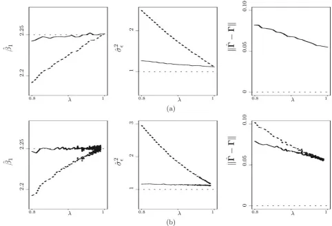
Withg=5,Figure 1depicts the MC average of ˆβ1and that of
ˆ
β1,Wversusλ(left panel), the same comparison for estimates of
σ2
(middle panel), and finallyˆ −and its naive counterpart
(right panel), whenu=σu2I3withσu2varying over a range to
produceλincreasing from 0.8 to 1 (inFigure 1(a)) or whenu
is equal to (inFigure 1(b))
h−1
⎡
⎣00..252 00..24 00.25.3 0.25 0.3 0.35
⎤
Figure 1. Averages of naive estimates (dashed lines) and averages of conditional score estimates (solid lines) across 1000 Monte Carlo replicates versus reliability ratioλfrom simulations in Section5.2, withg=5, (a)u=σu2I3, and (b)ugiven in (21). Dotted lines correspond to the true parameter values.
wherehvaries from 1 to 30. As a multivariate generalization of the reliability ratio, here we defineλ=tr{(x+u)−1x}/3,
wherexis the variance-covariance ofXl, which is equal toI3
in this experiment. Ashincreases from 1 to 30,ugiven in (21)
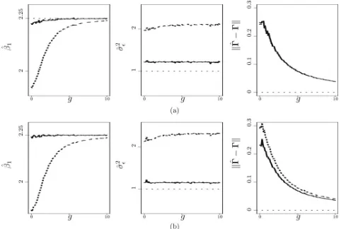
results inλvarying from 0.800 to 0.989.Figure 2presents the same comparisons between estimates versusgwhenλ=0.85, which is obtained by first settingu=(3/17)I3(inFigure 2(a)),
and second (inFigure 2(b)) settinguat ⎡
⎣ −00..191 −00..12 −00..152 −0.2 0.15 0.25
⎤
⎦. (22)
In both Figures1(a) and 2(a), with an isotropic diagonalu,
estimates of from two methods are very similar across the board, a phenomenon that reconciles with the comments made on (14) following Proposition 3.3. But when the assumption of isotropic and independent measurement error along all three coordinates is violated, as in both Figures1(b) and 2(b), ˆW
is more compromised by measurement error. As for the other parameters, Figure 1 suggests that naive estimates are more adversely affected by measurement error at lower levels ofλ, and the conditional score estimates are much more robust and accurate across differentλ. Moreover,Figure 2reveals that a more diffuseμX can substantially alleviate bias in the naive
estimates of the matching parameters due to measurement error.
This observation is consistent with the implication of (15) under Proposition 3.3.
6. APPLICATION TO REAL DATA
In what follows, we apply both naive OPA and the condi-tional score method to three real data examples, with the first two concerning two-dimensional configurations and the third considering three-dimensional configurations.
Figure 2. Averages of naive estimates (dashed lines) and averages of conditional score estimates (solid lines) across 1000 Monte Carlo replicates versusgfrom simulations in Section5.2, withλ=0.85 resulting from (a)u=(3/17)I3, and (b)ugiven in (22). Dotted lines correspond to the true parameter values.
the measurement error variance is unidentifiable in this study. As typically done in the measurement error literature whenσ2 u
cannot be estimated, we conduct a sensitivity analysis by setting
σ2
u at different values, and we monitor how the naive inference
compares with inference from the conditional score method at different assumed levels ofσ2
u. More specifically, at each time
point starting from age 14 days, we use data of all 18 rats to estimate σ2
x +σu2. Then we set σu2 at two levels to attain the
estimatedλequal to 0.5 and 0.9. From a practical standpoint,
λ=0.5 suggests severe measurement error contamination, and
[image:8.595.305.546.605.715.2]λ=0.9 implies moderate error contamination.
Figure 3 presents the estimated scale resulting from naive OPA and that from the conditional score method across seven time points at different levels ofλfor two randomly selected rats. The pictorial comparison betweenβˆ1andβˆ1,Whighlights
one key finding in Section3, which is that naive OPA tends to underestimate the scale parameter.
As pointed out by a referee, a natural extension of the above analysis is to embrace the longitudinal nature of the study and carry out a longitudinal size and shape analysis for the en-tire sample of 18 rats. For this extension, one may consider a longitudinal model in a very similar spirit as the longitudinal functional model proposed by Greven et al. (2010). This is be-yond the scope of our current study, and we provide a brief discussion in Appendix G in the supplementary materials on a
longitudinal model for configurations and its connection with the longitudinal functional model in Greven et al. (2010).
Example 2 (Brain templates). In this example, we consider
template matching in medical imaging where candidate tem-plates of brain images are generated by an automatic algorithm. For each axial MRI brain scan, eight landmarks are estimated on the corpus callosum according to a graphical template algo-rithm (Amit1997; Dryden2003), and the resulting candidate templates are subject to estimation error. Because, given one
Day
ˆβ1
0 50 100 150
11
.5
2
(a) Rat 1
Day
ˆβ1
0 50 100 150
11
.5
2
(b) Rat 2
11 11 111111111 11 1 111 111 1111111
2 2 1 112 211 1
1
11 11 1 1
1 11
4 4 3 4 4 4 3 4 3 3 1 1 11 1 1 1111
1 1 1 1 2 3 2 3 2
2 11
1 1 1 112 1 2 1 1 121 1
2 2
1
2 1 11 1111111111111111 11 1 111 111
2 2 1 112 211 1 1 11 1 11 1 1 1 1 4 4 3 4 4 4 3 4 3 3 1 1 11 1 1 1111 1 1 1 1 2 3 2 3 2 2 2 1 2 1 2222
1
2 1 1 1
221
2 2
1
2
1 1111
11 1 111 1 1 1 11 1 1 1 1 1 1 11111
1 2 1 1 12 21 1 1 1 1 1 1 11 1 11 1 3 4 3 4 4 4 3 4 3 3 1 1 1111 1 1 1 1
1 1 1 1 2 2 2 2 2 2 2 1 2
22222 1 2 1 2 1 2 2 2 2 2 1 2 1 1 1 1 111
1 1 1 1 1 1 1 1 1 1 1 1 1 1 11
1 1 1
2
22
212 2
1 1 1
1 11 11 1111
1 4 4 4 4 4 4 4 4 4 4
1 1 1 1
1 1 1 1 1 1 1 1 1 1 2 3 2 3 2 2 1 1 1 1111111 1 1 1 11 1
2
2 1
2 1 111 1 1111 111 11 1 1 1 1 1111111
2 2 1 112 211 1
1 1111
1
1 1 11
3 4 3 4 4 4 3 4 3 3 1 1 1111 1 1 1 1
1 1 1 1 2 3 2 2 2
2 11
1
11111 1
1 1 1 1 11 1
2 2 1 2 1 1 1 1 1 111 1 1 1 11 1 1 1 1 1 1 11111
1 2 1 112 211 1
1 11 11111 11 3 4 3 4 4 4 3 4 3 3 1 1 1111 1 1 1 1
1 1 1 1 2 2 2 2 2 2 2 2 2
22222 2 2 1 21 2 2 2 2 2 1 2 1 1 111 1 1 1 11 1 1 1 1 1 1 1111111
2 2 1 1 12 21 1 1 1 11 1111111 3 4 3 44 4 3 4 3 3 1 1 11 1 1 1111
1 1 1 1 2 3 2 2 2 2 2 1 1 12 122 1 2 1 1 1
221
2 2 1 2 1 111 1 1 1 11 1 1 1 1 1 1 1111111
2 2 1 1 12 21 1 1 1 11 11
1 1 1 1 1 3 4 3 4 4 4 3 4 3 3 1 1 11 1 1 1111
1 1 1 1 2 2 2 2 2 2 1 1 1 1 1 112 1 1 1 1 11 12
2 2 1 2 1 1 1 1 1 1 1 1 1 1 1 1
1 1 11
1 1 1 1 1 2 22 21 2 2 1 1 1 1 11111 1 11
1 4 4 4 44 4 4 4 4 4 1 1 1 1
1 1 1 1 1 1 1 1 1 1 2 3 2 3 2
2 11
1 1111111 1 1 1 11 1
2 2
1
2 1 1 11 1 1 1
1 11
1 1 11 11 1
1 1 1 2 2 2 21 2 2 1 1 1 1 11 1 1 1 1 1 1 1 4 4 44 4 4 4 4 4 4 1 1 1 1
1 1 1 1 1 1 1 1 1 1 2 3 2 3 2 2 1 1 1 1111111 1 1 1 11 1
2 2 1 2 1 1 1 1 1 1 1 1 1111 1112211
2 2 2 2122 1 1 1
1 1
111 1 1 1 1 1 2 4 2 4 4 4 2 4 2 2 1 1 1111 1 1 1 1
1 1 1 1 2 2 2 2 2 2 2 12 2 2 222 1 2 1 21 2 1 2 2 2 1 2 1 1 1 1 1 1 1 11 11 1222111
2 2 2 2 12 2 1 2 1 1
11 11 1 1 11 1 2 4 2 4 4 4 2 4 2 2 1 1 11 1 1 1111
1 1 1 1 2 2 2 2 2 2 2 12 22222
1 2 1 2 1 2 1 2 2 2 1 2 1 1 1 1 1 1 1 1112 22 221 2
2 2 2 2 12 2 1 2 1 1 11 1 1 1 1 1 1 1 2 5 2 5 5 5 2 5 2 2 1 1 11 1 1 1111
1 1 1 1 2 2 2 2 2 2 2 12 22222
2 2 2 2 2 2 2 2 2 2 2 2 1 1 1 1 1 1 1112 22 221 2
2 2 2 212 211 1 1 1 1 1 1 1 1 1 1 1 2 5 2 55 5 2 5 2 2 1 1 11 1 1 1111 1 1 1 1 2 2 2 2 2 2 2 2 2 2 2 222 2 2 2
2 22 2
2 2 2 2 2 1 1 1 1 1 2
2 2
2 11 121 2
2 2 2 2 12 2 1 1 1 1 111111
1 1 1 2 4 2 5 4 5 2 5 2 2 1 1 1111 1 1 1 1
1 1 1 1 2 2 2 2 2 2 2 12 22222
2 2 2 2 2 2 2 2 2 2 2 2
111 1 2
2 2
2 1 21 2 1 1 2 2 2 2 12 2 1 1 1 1 111111
1 1 1 2 4 2 4 4 5 2 4 2 2 1 1 11 1 11111
1 1 1 1 2 2 2 2 2 2 2 2 2 22222
2 2 2 2 2 2 2 2 2 2 2 2
11 1 2
2 2
2 1 21 2 1 1 2 2 2 2 12 2 1 1 1 1 11 11
1 1 1 1 1 2 4 2 4 4 5 2 4 2 2 1 1 11 1 11111
1 1 1 1 2 2 2 2 2 2 2 12 22 222 2 2 2 2 2 2 2 2 2 2 2 2
1 1 2
2 2 2 1 2 2 1 2 2 2 2 2 2 1 2 21 1 1 1 11 1 1 1 1 1 1 1 2 5 2 5 5 5 2 5 2 2 1 1 1111 1 1 1 1
1 1 1 1 2 2 2 2 2 2 2 2 2 22222
2 2 2 2 2 2 2 2 2 2 2 2 1 2 2 2 2 1 2 2 1 2 1 2 2 2 212 2 1 1 1 1 1
111 1 1 1 1 1 2 5 2 54 5 2 5 2 2 1 1 1111 1 1 1 1
1 1 1 1 2 2 2 2 2 2 2 12 2 2222
2 2 2 2 2 2 2 2 2 2 2 2 2 2 2 2 1 2 2 1 2 2 2 2 2 2 12 21 1 1 1 11 1 1 1 1 1 1 1 2 5 2 55 5 2 5 2 2 1 1 1111 1 1 1 1
1 1 1 1 2 2 2 2 2 2 2 2 2 22222
2 2 2 2 2 2 2 2 2 2 2 2 1 111 1 1 1 11
2 2 2 2
22
222 2
1 1 1 1 111 1 1 1
4
3
443 3
4 3
4 4
1 1 1111 1 1 1 1 1 1 1 1 1 3 2 3 1 2 1 1 1 11 11111111111
2 2 1 2 1 1111 1 11 2 2 2 2 22 22 2 2 1 1 1 1 111 1 1 1
4
3
443 3
4
3
4 4
1 1 11 1 1 1111 1 1 1 1 1 3 2 3 1 2 1 1 1 11 11111111111
2 2 1 2 1 111 1 1 1 2 2 2 2 22 22 2 2 11 1 1 11 11 1 1 4 3 4 3 3 3 43 4 4 1 1 11 1 1 1111 1 1 1 1 1 3 2 3 1 2 1 1 1 11 11111111111
2 2 1 2 1 111 1 1 2 2 2 2 22 2 2 2 2 11 1 1 11 11 1 1
4
3
433 3
4
3
4 4
1 1 1111 1 1 1 1 1 1 1 1 1 3 2 3 1 2 1 1 1 11 11111111111
2 2 1 2 1 111 1 2 2 2 222 2 1 2 1 1 1 1 1 111 1 1 1 4 3 4 4 4 4 4 4 4 4 1 1 11 1 1 1111 1 1 1 1 1 3 2 3 1 2 1 1 1 11 11111111111
2 2 1 2 1 111 2 22
222 222 2
11 1 1 11 11 1 1
4 3
433
4 4 3 4 4 1 1 11 1 1 1111 1 1 1 1
1 3 2 3 1 2 1 1 1 11 11111111111
2 2 1 2 1 11 2 2 2 2 22 2 2 2 2 11 1 1 111 1 1 1 4 3 43 3 4 4 3 4 4 1 1 11 1 1 1111 1 1 1 1
1 3 2 3 1 2 1 1 1 11 11111111111
2 2 1 2 1 1 2 2 2 2 22 21 2 1 1 1 1 1 11 11 1 1 4 4 4 44 4 4 4 4 3 1 1 1111 1 1 1 1 1 1 1 1 1 3 2 3 1 2 1 1 1 11 11111111111
2 2 1 2 1 2 2 2 2 2 2 2 2 2 2 1 1 1 1 111 1 1 1 4 3 4 3 3 3 4 3 4 4 1 1 11 1 1 1111 1 1 1 1 1 3 2 3 1 2 1 1 1 11 11111111111
2 2 1 2 2 2 2 2 22 22 2 2 11 1 1 11 11 1 1 4 4 44 4 4 4 4 4 4 1 1 1111 1 1 1 1 1 1 1 1 1 3 2 3 1 2 1 1 1 11 11111111111
2 2
1
2
111111111
2 2 2 2 2 2 2 2 2 2 5 4 5 4 4 4 5 4 5 5 2 2 2 2 2 2 2 2 2 2 2 2 2 2 2 3 2 3 2 2 2 2 2 2 2 2 2 2 2 2 2 2 2 2 2 2 3 3 2 3 11111111
2 2 2 2 2 2 2 2 2 2 5 4 5 4 4 4 5 4 5 5 2 2 2 2 2 2 2 2 2 2 2 2 2 2 2 2 2 2 2 2 2 2 2 2 2 2 2 2 2 2 2 2 2 2 2 2 3 3 2 3 1111111
2 1 2 2 2 2 2 2 2 1 5 4 5 4 4 4 5 4 5 5 2 2 2 2 2 2 2 2 2 2 2 2 2 2 2 3 2 3 2 2 2 22 2 2 2 2 2 2 2 2 2 2 2 2 2 3 3 2 3 111111
2 2 2 2 2 2 2 2 2 2 5 4 5 4 4 4 5 4 5 5 2 2 2 2 2 2 2 2 2 2 2 2 2 2 2 3 2 3 2 2 2 2 2 2 2 2 2 2 2 2 2 2 2 2 2 2 3 3 2 3 111 11 1 1 1 2 2 2 2 2 2 1 5 4 5 4 4 4 5 4 5 5 2 2 2 2 2 2 2 2 2 2 2 2 2 2 2 3 2 3 2 2 2 2 2 2 2 2 2 22 2 2 2 2 2 2 2 3 3 2 3 1111
2 2 2 2 2 2 2 2 2 2 5 4 5 4 4 4 5 4 5 5 2 2 2 2 2 2 2 2 2 2 2 2 2 2 2 2 2 2 2 2 2 2 2 2 2 2 2 2 2 2 2 2 2 2 2 2 3 3 2 3 1 1 1
2 2 2 2 2 2 2 2 2 2 5 4 5 4 4 4 5 4 5 5 2 2 2 2 2 2 2 2 2 2 2 2 2 2 2 2 2 2 2 2 2 2 2 2 2 2 2 2 2 2 2 2 2 2 2 2 3 3 2 3 1 1 1 1 1 1 1 1 1 21 1 5 4 5 4 4 4 5 4 5 5 2 2 2 2 2 2 2 2 2 2 2 2 2 2 2 3 2 3 2 2 2 2 2 2 2 2 2 22 2 2 2 2 2 2 2 3 3 2 3 1 2 2 2 2 2 2 2 2 2 2 5 4 5 4 4 4 5 4 5 5 2 2 2 2 2 2 2 2 2 2 2 2 2 2 2 2 2 2 2 1 2 2 2 2 2 2 2 22 2 2 2 2 2 2 2 3 3 2 3 1 1 1 1 1 1 1 2 2 1 5 4 5 4 4 4 5 4 5 5 2 2 2 2 2 2 2 2 2 2 2 2 2 2 2 3 2 3 2 2 2 2 2 2 2 2 2 22 2 2 2 2 2 2 2 3 3 2 3 1 1 1 1 1111 1
4
3
4 43
4
4 4
3
4
1 1 11 1 11111
1 1 1 1 2 3 2 3 2 2
11 111111111
1 1 1 1 1 2 2 1 2 1 1 1 1 111 1
4 3 3 4 4 4 3 4 3 4 1 1 11 1 11111
1 1 1 1 2 2 2 2 2 2
11 111111111
1 1 1 1 1 2 2 1 2 1 1 1 1111
3 4 3 4 4 4 3 4 3 3 1 1 11 1 11111
1 1 1 1 2 2 2 2 2 2 11 1 12 1 1 1 11111
111
2 2 1 2 1 1 1 1 11
4 4
34 4
4 3 4 3 3 1 1 11 1 1 1111
1 1 1 1 2 3 2 2 2 2 11 111111111
1 1 1 1 1 2 2 1 2 1 1 1 1 1 4 3 4 4 3 4 4 4 4 4 1 1 11 1 1 1111
1 1 1 1 2 3 2 3 2 2 1 1 1 11 11 111111111
2 2 1 2 1 1 1 1 4 3 4 4 3 4 4 4 4 4 1 1 11 1 1 1111 1 1 1 1 2 3 2 3 2 2 1 1 1 11 11 111111111
2 2 1 2 1 1 1 4 3 4 4 3 4 4 4 4 4 1 1 11 1 11111
1 1 1 1 2 3 2 3 2 2 1 1 1 11 11 111111111
2 2 1 2 1 1 4 4 4 4 4 4 4 4 4 4 1 1 11 1 1 1111
1 1 1 1 2 3 2 3 2 2 1 1 1 11 11 111111111
2 2 1 2 1 4 4 4 4 4 4 4 4 3 4 1 1 11 1 1 1111 1 1 1 1 2 3 2 3 2 2 1 1 1 11 11 111111111
2 2 1 2 3 3
343
4
3 4
3 3
1 1 11 1 11111
1 1 1 1 2 2 2 2 2 2
1111 1 1 11 1 1 1 1 1 1 1 1 2 2 1 2 2 1 2 2 2 1 2 1 1 3 3 3 3 3 3 3 3 3 3 3 3 3 3 4 5 4 5 4 4 3 2 3 3 3 333 2 3 3 3 3 3 3 3 4 4 3 4 2 111
2 1 2 2 4 4 4 4 4 4 4 4 4 4 4 4 4 4 4 6 4 6 4 4 4 4 4 44 444 4 4 4 4 4 4 4 5 5 5 4 4 2 2 2 1 2 1 1 3 3 3 3 3 3 3 3 3 3 3 3 3 3 4 5 4 5 4 4 3 2 3 3 3 33 3 2 3 3 3 3 3 3 3 4 4 3 4 1 1 2 1 2 2 4 5 5 5 4 5 4 4 5 4 4 4 5 5 5 6 5 6 5 5 4 4 4 4 44 4 4 4 4 4 5 4 5 4 5 5 5 5 5 1 2 1 2 2 4 4 4 4 4 4 4 4 4 4 4 4 4 4 4 6 4 6 4 4 4 4 4 44 444 4 4 4 5 4 4 4 5 5 5 4 4 2 1 2 2 5 5 5 5 4 5 5 5 5 5 5 4 5 5 5 6 5 6 5 5 4 4 4 444 4 4 4 4 5 5 5 5 5 5 5 5 5 5 2 1 1 4 4 4 4 4 4 4 4 4 4 4 3 4 3 4 5 4 5 4 4 3 3 3 3 3 3 3 3 3 3 4 4 4 4 4 4 4 4 4 4 2 2 4 5 5 5 4 5 4 4 5 4 4 4 5 5 5 6 5 6 5 5 4 4 4 44 4 4 4 4 4 4 5 4 5 4 5 5 5 5 5 1 4 4 4 4 4 4 4 4 4 4 4 3 4 3 4 5 4 5 4 4 3 3 3 3 3 3 3 3 3 3 4 4 4 4 4 4 4 4 4 4 4 4 4 4 4 4 4 4 4 4 4 4 4 4 4 5 5 5 4 5 3 3 3 3 33 3 3 3 3 4 4 4 4 4 4 4 4 4 4 1 1 1 1 11 1 1 1 1 1 1 1 2 2 2 2 2 2 1 1 1 11 11212 1 1 11 12
2
2 1
2
1 111 1111 1 1 1 1
2 3 2 3 2 2 1 1 1 11 11111111111
2 2
1
2
1 1 1111 1 1 1 1 1
2 3 2 3 2 2 1 1 1 11 11111111111
2 2
1
2
1 11111 1 1 1 1
2 3 2 3 2 2 1 1 1 11 11111111111
2
2 1
2
1 1 111 1 1 1 1 2 2 2 2 2 2 2 112222221 1 21
221
2 2
1
2
1 1 1 1 1 1 1 1
2 3 2 3 2 2 1 1 1 11 11111111111
2 2 1 2 1 1 1 1 1 1 1 2 2 2 2 2 2 1 1 1 11 1121 1 1
1 1 1 1 1 2 2 1 2 1 1 1 1 1 1 2 3 2 3 2 2 1 1 1 11 11111111111
2 2
1
2
1 1 1 1 1
2 3 2 3 2 2 1 1 1 11 11111111111
2 2 1 2 1 1 1 1 2 2 2 2 2 2 2 121222221 1 21
221
2 2
1
2
1 1 1
2
3 2
3 2
2 1 1111
11 1 1 1 1 1 1 11 1
2 2 1 2 1 1 2 3 2 3 2 2 1
1 111 11 1 1 1 1 11 1
1 1 2 2 1 2 1 2 3 2 3 2 2 1 1 1 1 1 11 1 1 1 1 11 1
1 1 2 2 1 2 2 3 2 3 2
2 11
1 1 1 11 1 1 1 1 1 1 1 1 1 2 2 1 2 3 2 3 1 2 1 11111 1 1 1 1 1 11 1 1 1 2 2 1 2 4 1 4 4 3 3 3 3 3 3 3 3 3 3 3 3 3 3 3 3 33 3 3 4 1 1 2
2 22
2 2 2 22 2 1 1 1 1 1 1 2 2 1 2 4 4 3 3 3 3 3 3 3 3 3 3 3 3 3 3 3 3 33 3 3 2 1 1 1 1 1 1 1 11 1 1 1 1 1 1 1 22 1 2 2 2 2 2 2
222
2 2 1 1 1 1 2 1 2 2 1 2 11 1 1 11 11 1 1 1 1 1 1 1 2 2 1 2 1 1 11 1 111
1 1 1 1 1 1 2 2 1 2 1 1111 111
1 1 1 1 1 2 2 1 2
1111 1 1
1 1
1 111
2 2
1
2 1111 1 1 1 1 1 1 1 2 2 1 2 1111 1 1 1 1 1 1 2 2 1 2 111 1 1 1 111
2 2 1 2 1 1 1 1 1 111
2 2 1 2 1 1 1 1 1 1 1 2 2 1 2 1 11 111
2 2
1
2 1 1 1 11
2 2 1 2 1 1 1 1 2 2 1 2 1 1 1 2 2 1 2 1 1 2 2 1 2 1 2 2 1 2 2 2 1 2 1 2 1 2 1 2
ˆβ1
,
W
/
ˆβ1
ˆ β1 0.6 0.8 0.94 0.96 0.98 1
1 1.2 1.4 1.6 1.8
Figure 4. Ratio ofβ1ˆ,Woverβ1ˆ versusβ1ˆ based on 100 brain templates, resulting in 4950 pairs, in Example 2. Estimated standard errors ofβ1ˆ (s.e.) associated with different numerical symbols are: s.e.∈(0,0.1) for “1,” s.e.∈[0.1,0.5) for “2,” s.e.∈[0.5,1) for “3,” s.e.∈[1,2) for “4,” s.e.∈[2,3) for “5,” and s.e.∈[3,4.21) for “6.”
slice of the brain scan, these candidate templates can be viewed as error-contaminated measures of the same underlying structure in the corpus callosum, the true scale parameter when matching one template onto the other, while appropriately accounting for measurement error, is equal to one. Using all available 604 can-didate templates corresponding to the same slice of brain scan, we obtain ˆσu2≈0.002 and ˆσx2+σˆu2≈0.015, yielding an
esti-mated reliability ratio as 0.860. Then we choose a particular pair of templates asYandW. MatchingWontoYvia naive OPA yields the estimated scale as 0.951 (0.061) and the estimated ro-tation as 2.116◦(2.956), with sandwich standard error estimates in parentheses, and the counterpart conditional score estimates are 0.999 (0.062) and 2.116◦(2.947). With such a small number of landmarks (K =8), high variability in these estimates is in-evitable. Although we cannot conclude statistically significant discrepancy between the naive scale estimate and conditional score estimate (with the high variability in estimates), we ob-serve across all 182,106 pairs (from 604 templates withYand Wassigned at random for each pair) that the former is never larger than the latter.Figure 4depictsβˆ1,W/βˆ1versusβˆ1
when matching 4950 pairs resulting from the first 100 templates.
Example 3 (Face data). Evison et al. (2010) analyzed three-dimensional facial images of healthy volunteers, which were collected using a Geometrix FaceVisionR FV802 Biometric Camera (ALIVE Tech, Cumming, GA). To demonstrate the conditional score method for three-dimensional shape data in comparison with naive OPA, we implement these two methods using data from one volunteer, whose facial configuration con-sisting of 61 landmarks was measured twice by each of the two operators in the study.
More specifically, denote byW1,w andW2,w the two
repli-cate measures for this volunteer’s face collected by one operator, and byYa facial configuration of the same volunteer measured by the other operator. Using the duplicate measures,W1,wand
W2,w, and applying the method related in Section4.3, we obtain
ˆ
σu2≈0.007. This estimate of the measurement error variance, in contrast to the estimate ofσ2
x +σu2(≈5.216), results in the
esti-mated reliability ratio equal to 0.999, suggesting minimal error contamination in the observed facial images. This is also implied by Evison et al. (2010), who stated that the three-dimensional coordinates of landmarks were collected with high precision us-ing a software tool. The estimated scale resultus-ing from matchus-ing W1,wontoYusing naive OPA and the conditional score
esti-mate are 0.988 (0.006) and 0.990 (0.006), respectively, with the corresponding estimated standard errors in parentheses. As ex-pected when measurement error is scarce, these two estimates are very similar. To simulate a scenario with slightly more error contamination as expected from CCTV cameras in the field, we add isotropic measurement error toW1,wto reduce the
reliabil-ity ratio to 0.9, and repeat the two analyses using the further contaminated configuration. This round of analyses yields the naive estimate of the scale as 0.845 (0.020) and the conditional score estimate as 0.920 (0.024), which demonstrates that naive OPA leads to an attenuated scale estimate.
7. DISCUSSION
We have shown theoretically and empirically that compar-isons of two error-contaminated configurations via naive OPA can be misleading, with the adverse effects of measurement error mostly manifested in the attenuated scale estimation. Be-sides the severity of error contamination, the interplay of sev-eral factors that affect the degree of deterioration in inference from naive OPA is revealed in our bias analyses in Section3. One noteworthy finding is that ignoring measurement error does less harm when the unobserved true configuration consists of more diffuse landmarks. Comforting as this finding sounds, one may not know with absolute certainty if the true configuration has landmarks diffuse enough to counteract measurement error in one particular application. The proposed conditional score method that accounts for measurement error and yields consis-tent inference for all parameters of interest is a valuable addition to the methodology available for size and shape analyses.
Formulating the measurement error models for shape data using complex/quaternion random variables allows us to de-rive the conditional scores in ways that are similar to those employed in the context of real-value linear measurement er-ror models. However, although it is assumed in most real-value regression analyses that (Yl, Xl, Wl) are independent across
l=1, . . . , K, it is more natural to view (Yl, Xl, Wl) correlated