to Tackle Multiobjective Problems With
Recurring Fitness Landscapes
Rodrigo Lankaites Pinheiro1,2, Dario Landa-Silva2, Wasakorn Laesanklang3, and Ademir Aparecido Constantino4
1 Webroster Ltd., PE1 5NB, Peterborough, UK
2 ASAP Research Group, School of Computer Science, University of Nottingham, UK
3 Department of Mathematics, Faculty of Science, Mahidol University, Thailand
4
Departamento de Inform´atica, Universidade Estadual de Maring´a, Maring´a, Brazil
Abstract. Many real-world applications require decision-makers to as-sess the quality of solutions while considering multiple conflicting objec-tives. Obtaining good approximation sets for highly constrained many-objective problems is often a difficult task even for modern multiobjec-tive algorithms. In some cases, multiple instances of the problem sce-nario present similarities in their fitness landscapes. That is, there are recurring features in the fitness landscapes when searching for solutions to different problem instances. We propose a methodology to exploit this characteristic by solving one instance of a given problem scenario using computationally expensive multiobjective algorithms to obtain a good approximation set and then using Goal Programming with efficient single-objective algorithms to solve other instances of the same problem scenario. We use three goal-based objective functions and show that on benchmark instances of the multiobjective vehicle routing problem with time windows, the methodology is able to produce good results in short computation time. The methodology allows to combine the effectiveness of state-of-the-art multiobjective algorithms with the efficiency of goal programming to find good compromise solutions in problem scenarios where instances have similar fitness landscapes.
Keywords: multi-criteria decision making, goal programming, Pareto optimisation, multiobjective vehice routing
1
Introduction
can choose the preferred solution(s). It is often useful to use problem domain knowledge during the optimisation in order to obtain better sets of compromise solutions. For example, in the context of continuous multiobjective optimisation problems, Giagkiozis and Fleming (2014) estimated Pareto fronts to then obtain values for the decision variables of interesting solutions. Their technique allows to focus the search in sub-regions of the objective space. Another example is the work by Feliot et al. (2016) using a Bayesian model to learn computationally expensive objective functions to then use the estimation model to explore the search space more quickly.
The multiobjective vehicle routing problem with time windows (MOVRPTW) is a well-know difficult combinatorial optimisation problem that arises in many real-world logistic scenarios (Toth and Vigo, 2002). This problem refers to creat-ing a plan for a fleet of identical vehicles to take goods from a depot and deliver them to customers at various locations. Each customer has certain demand level that needs to be satisfied within a specified time window. Objectives usually con-sidered in the MOVRPTW include among others, the minimisation of number of vehicles and the minimisation of total travel distance by all vehicles.
Due to the high number of constraints and objectives in MOVRPTW sce-narios, even state-of-the-art multiobjective algorithms struggle to find good ap-proximations to the Pareto optimal front within reasonable computation time. In logistic scenarios where problems like MOVRPTW arise, it is often the case that problem instances corresponding to a different planning periods share parts of the same data. For example, the same or very similar set of vehicles might be available in each planning period. Also, there might be a set of recurring customer orders that need to be satisfied in the different planning periods. This results in the different problem instances presenting recurring features in their fit-ness landscapes. Other problems like timetabling and personnel scheduling may also have instances with recurring features resulting in similar fitness landscapes (η-dimensional surface representing the Pareto front, whereη is the number of objectives).
Previous work proposed a technique to analyse and visualise complex objec-tive relationships and fitness landscapes in multiobjecobjec-tive problems (Pinheiro et al., 2015, 2017). Later, Pinheiro et al. (2018) introduced a methodology to exploit the recurring similarity between instances of a multiobjective workforce scheduling and routing optimisation problem, in order to solve instances of the same problem scenario more efficiently. In this methodology, a pilot problem instance is solved first using some effective (but not necessarily computationally efficient) multiobjective algorithm to produce an approximation to the Pareto optimal set. Such approximation set is given to the decision-maker so thattarget
to facilitate informed decision-making when searching solutions to multiobjec-tive problems. Experiments in this paper are conducted on a set of benchmark instances of the MOVRPTW provided by Castro-Gutierrez et al. (2011).
Section 2 outlines the multiobjective vehicle routing problem with time win-dows considered here while Section 3 outlines goal programming. Section 4 de-scribes the proposed methodology and Section 5 presents the experimental con-figuration. Sections 6 and 7 present and discuss the results. Section 8 concludes the paper and suggests related future research.
2
Multiobjective Vehicle Routing Problem with Time
Windows
A Multiobjective Vehicle Routing Problem with Time Windows (MOVRPTW) is defined on a graphG= (V, E) whereV is the set of vertices representing the depot (vertex 0) and the customers (vertices 1. . . n) where each customer has a demand pi (i = 1, . . . , n). There are h identical vehicles available, each one with capacity Q. In this MOVRPTW,h is considered large enough so that as many vehicles as needed are available to create the routing plan. A set of routes served by the set of vehicles should be created in order to satisfy all demands from all customers. All routes must start and end in vertex 0. The edge set E denotes all possible connections between all vertices. Each edge from vertexito vertexj has an associated cost, denoted bycij, that represents distance or time for a vehicle to travel between verticesiandj. Each customerimust be served during their corresponding time window [ai, bi]. A waiting time is incurred if a vehicle arrives at timet < ai and hence it must wait until the start of the time window to serve the customer. A delay time is incurred if a vehicle arrives at timet > ai and hence it must start serving the customer immediately. Once the vehicle starts serving the customer, it stays there forstime until the delivery is completed, this is known as the service time.
Castro-Gutierrez et al. (2011) proposed a benchmark set of instances for the MOVRPTW with five minimisation objectives: number of vehicles (Z1), total travel distance by all vehicles (Z2), makespan or travel time of the longest route (Z3), total waiting time for all vehicles (Z4), and total delay time for all vehicles (Z5). They designed their instances based on different characteristics of the problem and each instance is a combination of these features. The features that constitute a problem instance in these benchmarks are:
– Number of customers: 50, 150 and 250 customers.
– Time window:five different profiles (tw0, tw1, tw2, tw3, tw4) of time win-dows across a planning period of eight hours. These profiles are defined in terms of minutes from the start of the planning period 0 = 8:00 am, 480 = 4:00 pm, etc.). These five time-window profiles are defined as follows:
• tw0: [0,480], all customers can be served at any time in the day. • tw1: [0,160],[160,320],[320,480], refers to three types of customers
• tw2: [0,130],[175,305],[350,480], also refers to three types of customers as in profiletw1 but with shorter time windows.
• tw3: [0,100],[190,290],[350,480], also refers to three types of customers as in profiletw1 but with longer time windows.
• tw4: includes all time-windows from tw0, tw1, tw2 and tw3, each cus-tomer has one of the 10 time window types in the previous profiles. – Demand types: three types of demand (10, 20, 30) uniformly distributed. – Vehicle capacity:the capacity of the vehicles is calculated according to aδ parameter such thatQ=D+δ/100(D−D) whereDis the maximum single demand among all customers andD is the sum of all customer demands. The dataset considers threeδvalues (δ0 = 60,δ1 = 20, δ2 = 5).
– Service time:three values of service time (10, 20, 30) uniformly distributed. For more details of the MOVRPTW described above and a comprehen-sive study on the multiobjective nature of the problem, please refer to Castro-Gutierrez et al. (2015). There are 45 problem instances and a generator avail-able from https://github.com/psxjpc/MOVRPTW-Generator. The technique to analyse objective relationships described in Pinheiro et al. (2017) was applied to these problem instances and results indicate that indeed they have similar fitness landscapes. This is the case even for instances that have different time window profiles, vehicle capacity and the number of customers. However, in this work, we split the 45 problem instances into three datasets according to the number of customers. This decision was taken because even though the fitness landscapes are similar, the scale of the objective values vary considerably according to the number of customers. Therefore, we have 3 datasets each with 15 problem in-stances, the set VRP-50 with 50 customers, the set VRP-150 with 150 customers and the set of VRP-250 with 25 customers.
3
Goal Programming
Without loss of generality, a multiobjective optimisation problem can be written as minimise F(x) = (f1(x), f2(x), ..., fn(x)) subject to x ∈ S, where x is a solution,S is the set of feasible solutions, n is the number of objectives in the problem, F(x) is the image of xin the k-objective space and eachfi(x) is the value of objective i in solution x. For two solutions xand y, it is said that x dominatesy, if∀i:fi(x)≤fi(y) and∃j :fj(x)< fj(y). Moreover,xis said to be
Pareto Optimal if it is not dominated by any other feasible solution. Then, the aim is to find the set ofPareto Optimal solutions usually calledPareto Set. This set contains a number of non-dominated points in the objective space creating thePareto Front.
the goals is minimised. In order words, goal programming is about establishing a target for each objective and then searching for a solution with objective val-ues as close as possible to those targets. There are three types of goals in goal programming (Kornbluth, 1973):
– Lower bound: defines a lower value for an objective such that solutions that fall below the lower value are penalised.
– Upper bound: defines an upper value for an objective such that solutions that present higher values than the upper value are penalised.This is the type of goals in the optimisation problem considered here, due to the minimisation nature of all objectives.
– Strict bound: defines a specific target value such that solutions that present values above or below are penalised. This is applicable when obtaining a solution with a specific target value for a given objective is essential. For example, in the case that solutions using exactlyhnumber of vehicles were required in the MOVRPTW.
Once the goals for each objective are set, goal programming techniques derive problem models (LP, MIP, etc.) to find solutions that reach (or are close enough to) the target goals. Several strategies, or goal programming variants, have been presented in the literature. We briefly review the three most widely employed variants (Jones and Tamiz, 2016):
– Weighted GP (Romero, 1991): used when the decision maker is able to assign an importance weight to each goal. The objective function for the problem is then a weighted sum of the deviations from the goals.
– Lexicographic GP: when weighting the goals is difficult, but the decision maker is able to prioritise them, the lexicographic GP technique is commonly applied (Tamiz et al., 1995). The deviations to the target goals are minimised according to defined priority levels such that deviations from a higher level goal are considered infinitely more important that deviations from a lower level goal.
– Chebyshev GP(Flavell, 1976): consists of minimising the maximum weighted normalised deviation from all the goals, hence promoting solutions that are well-balanced regarding the achievement of the target values.
The weighting and lexicographic methods are considered ‘a priory’ approaches in the sense that the decision maker should set a ranking between the objectives before conducting the search for solutions. This is not the case in the Chebyshev method which is an ‘a posteriori’ method because it seeks solutions that are well-balanced in the attainment of all goals so that the decision maker can chose afterwards. In this paper, it is assumed that the decision maker is able to choose a preferred solution from a set of trade-off solutions, instead of being able to establish weights or ranking between the multiple objectives. Hence, only the Chebyshev technique is used later in this work.
when the goals are ‘pessimistic’ and the objectives can be easily achieved. Sev-eral methods are proposed to address the issue. Most methods rely on extra information from the decision maker in order to promote the further improve-ment of certain objectives (Tamiz et al., 1999). Other methods involve extending the search after the solution is found by the goal programming in order to find dominating solutions (Hannan, 1980).
Works in the literature usually describe the application of goal program-ming using exact methods (Jones and Tamiz, 2010, 2016). However, many works exist where metaheuristics are employed to solve goal programming models. Baykasoglu (2005) presents a simulated annealing approach to tackle several test problems of preemptive goal programming. Mishra et al. (2006) employ a fast converging simulated annealing algorithm to solve a machine-tool selection and operation allocations problem with fuzzy variables. Ghoseiri and Ghannad-pour (2010) propose a genetic algorithm to tackle a goal programming model for the vehicle routing problem with time windows and Leung (2007) presents a genetic algorithm to tackle a goal programming model for a transportation planning problem with three objectives. Goal programming is a sound approach to tackle the MOVRPTW considered here becasue this technique has been suc-cessfully applied to related scheduling and routing problems. For example, it has been applied to nurse scheduling (Azaiez and Al Sharif, 2005) (Musa and Saxena, 1984) and to a version of the vehicle routing problem with soft time-windows (Calvete et al., 2007).
4
The Efficient GP Methodology
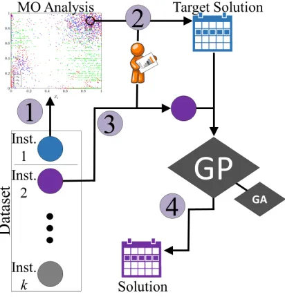
Figure 1 shows the overall concept of the methodology which was originally proposed in Pinheiro et al. (2018). Each of the steps is explained below in ref-erence to the MOVRPTW tackled in this paper. The overall idea is to find a set of compromise solutions for a representative instance of the multiobjective problem in hand. The decision maker then selects from this set a solution that exhibits the desirable qualities in respect of the various objectives, without the need to set weights or priorities for the objectives. The objective values in the selected solutions are set as the targets for goal programming when searching for solutions to the other problem instances (e.g. routing plans for other days in the same problem scenario).
1. Apilot instance from the dataset with recurring fitness landscape is selected by the decision-maker and solved using multiobjective algorithms to obtain the best possible non-dominated approximation set.
2. The decision-maker chooses a preferred solution t from the obtained non-dominated set. This chosen solution is known as thetarget solution and its objective-vector is denoted by
Fig. 1.Overview of the methodology as in Pinheiro et al. (2018). The numbered steps are explained in the main text.
3. Each other instance in the dataset can now be solved with a faster single-objective algorithm using a modified single-objective function (goal programming variant) aiming to reach the target objective vector.
4. The final solution obtained in Step 3 is presented to the decision maker. The overall advantage of this approach is that Step 1, which is typically computationally expensive, needs to be executed only once for a given rep-resentative instance in the problem scenario. Then, other problem instances can be solved faster after the target solution is chosen.
The modified objective function of Step 3 has an important role in the methodology as it establishes the way in which the search will aim to attain the goals. Three approaches are used here for determining the objective func-tion. The first one is the well known Chebyshev approach. The second one is to derive a weight-vector from the target solution and the approximation set of the pilot instance. The third approach minimises the Euclidean distances to the target objective-vector.
4.1 Chebyshev Goal Programming
to achieve (i.e. the target goal is too optimistic), the quality of that objective can be a bottleneck for the other objectives because the search will solely focus on improving that objective. We define the Chebyshev objective function for the MOVRPTW as follows:
Minimise λ (1)
Subject to Z1 Zt 1
≤λ (2)
Z2 Zt 2
≤λ (3)
Z3 Zt 3
≤λ (4)
Z4 Zt 4
≤λ (5)
Z5 Zt 5
≤λ (6)
The Chebyshev objective function given by Eq. (1) is used as the objective function for the MOVRPTW. The main objective is now to minimise λ, thus finding a well-balanced solution regarding reaching the target values. If all targets are reached,λcan assume fractional values and a solution that shows balanced improvements on all objectives may be obtained.
4.2 Derived Weight Vector
One problem with the Chebyshev approach is that it does not guarantee Pareto efficiency. However, the optimal solution for a weighted sum objective function (where weights are not simultaneously null) is always Pareto efficient. To derive a weight vector from the target solution, we first convert the approximation set of the pilot instance into a system of linear inequalities. Considering that the approximation set is composed ofkobjective-vectors (Z1,Z2,. . .,Z5), the linear inequalities system can be defined as follows where the aim is to determine the values ofw= (w1, w2, w3, w4, w5):
wZt≤wZ1
wZt≤wZ2
. . .
wZt≤wZk
There is no guarantee that the system of linear inequalities has a solution if the fitness landscape is non-convex, i.e. if no set of weights can be set to achieve some points in the Pareto optimal front. Therefore, instead of finding a solution for the system, we aim to find a weight vectorwthat satisfies the largest number of inequalities. Hence, we define the problem of finding the best weight vector as the following MIP (mixed-integer programming) minimisation problem.
Minimise
k
X
j=1
xj (8)
Subject to
wZt−wZj≤M xj j= 1, . . . , k (9)
wi∈(0,1], xj binary
(
i= 1, . . . ,5 j= 1, . . . , k (10)
The objective function in Eq. (8) aims to find a weight vectorw that min-imises the number of linear inequalities in (7) which do not fulfill the condition
wZt≤wZiexpressed by constraint (9),M is a large constant. Constraint (10) guarantees that zero cannot be chosen as a weight-value (to avoid criteria being removed).
Finally, the weight vector w obtained from the MIP model is used in the objective function for the MOVRPTW as given by Eq. (11).
Minimise 5 X
i=1
wiZi (11)
4.3 Euclidean Distances
Henceforth, the objective function in Eq. (12) becomes the objective function for the optimisation problem in hand.
Minimize (
z if z >
−z0 otherwise (12)
where z= v u u t 5 X i=1
zi (13)
z0= v u u t 5 X i=1 z0 i (14)
zi=
(
(Zi−Zit)2 if Zi> Zit
0 otherwise (15)
zi0=
(
(Zi−Zit)
2
if Zi≤Zit
0 otherwise (16)
In summary, when the Euclidean distances of the objectives that are worse than the target vector are larger than the given parameter, the objective func-tion consists of minimising the Euclidean distances (z). Otherwise, whenz≤, the objective consists of maximising the distances for the objectives that are better than the target solution (z0). Thus, if the solution has not reached the
target, the objective function attempts to close the gap to the target. If the solution is close or better than the target, the objective function attempts to further improve it.
5
Experimental Configuration
We applied the proposed methodology to the MOVRPTW datasets. The in-stances with δ0 and tw4 (50-δ0-tw4, 150-δ0-tw4, 250-δ0-tw4 were arbitrarily selected as pilot instances (Step 1 of methodology). Once the Pareto approxima-tion sets were obtained,k= 15 target vectors were randomly selected (uniformly distributed) from each approximation set and the same target vectors were used for the Derived Weight Vector (WV) objective function, the Euclidean Distances (ED) objective function, and the Chebyshev (CV) objective function.
This study utilises NSGA-II (Deb et al., 2002) as the Pareto-based algorithm and MOEA/D (Zhang and Li, 2007) as the decomposition-based one. Thus,for each problem instance the approximation set was obtained (Step 1 of methodol-ogy) as described below. The number of solution vectors obtained for each pilot instance was 168 for 50-δ0-tw4, 215 for 50-δ0-tw4 and 206 for 250-δ0-tw4.
1. run both the NSGA-II and MOEA/D for one million objective evaluations on each possible bi-objective vector (Z1,Z2), (Z1, Z3),. . . (Z4,Z5); 2. run both the NSGA-II and MOEA/D for one million objective evaluations
on each possible three-objective vector (Z1,Z2,Z3), (Z1, Z2,Z4), . . . (Z3, Z4, Z5);
3. run both the NSGA-II and MOEA/D for one million objective evaluations on each possible four-objective vector (Z1,Z2,Z3,Z4), (Z1,Z2,Z3,Z5),. . . (Z2,Z3,Z4,Z5);
4. create an archive composed of the non-dominated solutions found in the previous three steps;
5. generate a population of individuals where half of the elements are randomly generated and the other half are randomly drawn from the archive built in the previous step;
6. run both the NSGA-II and MOEA/D four times each, for two million objec-tive evaluations, using the initial population generated in the previous step and the five-objective vector; and
7. compile an approximation set with all non-dominated solutions found in all steps.
Br¨aysy and Gendreau (2005) survey the literature on vehicle routing prob-lem with time windows and show that genetic algorithms are well suited for that problem. Also, our early experiments showed that these algorithms present good enough solutions on these datasets and are simple enough to allow easy replication by other researchers. Hence, for Step 3 of the methodology, the other instances of the MOVRPTW are tackled with a straightforward genetic algo-rithm (GA) using a direct integer encoding of solutions, uniform crossover, 500 individuals population with a 5% elite being kept across generations and a tour-nament of two individuals employed for the selection mechanism.
6
Experimental Results
First, we show the effectiveness of the derived weight vector obtained from the MIP model in Eqs. (8)–(10). The effectiveness of a weight vector w is given by the percentage of solutions (in the approximation set for the pilot instance) in which wZt ≤ wZi, i = 1, . . . ,5. Hence, if the effectiveness is 100%, it means that the MIP model found a solution for the inequalities system in Eq. (7).
50-δ0-tw4 150-δ0-tw4 250-δ0-tw4 90%
92% 94% 96%
Pilot Instance
W
eigth
V
ector
Effectiv
[image:12.612.184.428.113.251.2]eness
Fig. 2. Average percentage of the solutions in the approximation set of each pilot instance in the MOVRPTW datasets such thatwZt≤wZi.
Hence, in all cases, the MIP model provided good weight vectors to be used by the WV objective function.
Next, we show the results for each group of instances (for 50, 150 and 250 customers) in three charts. Thetarget achievement chart displays the percentage of solutions, in the given dataset, that achieved the target value in each objective. Thegap to target chart contains the average gap to the target solutions for the solutions that did not reach the target. Finally, the overall comparison chart displays the average quality of solutions where positive values indicate that, on average, the solutions found are better than the target solution and negative values indicate that the solutions are worse than the target solution.
Z1 Z2 Z3 Z4 Z5
60% 80% 100%
WV ED CV
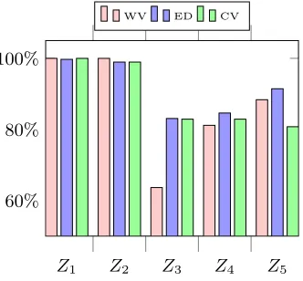
[image:12.612.227.393.487.641.2]Figures 3–5 display the results of applying the implemented GA with all three objective functions (WV, ED and CV) to the other instances of dataset VRP-50. Results comprise the average values of eight runs for each target vector of each problem instance for each objective function.
Z1 Z2 Z3 Z4 Z5
0% 2% 4% 6%
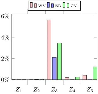
[image:13.612.223.392.183.346.2]WV ED CV
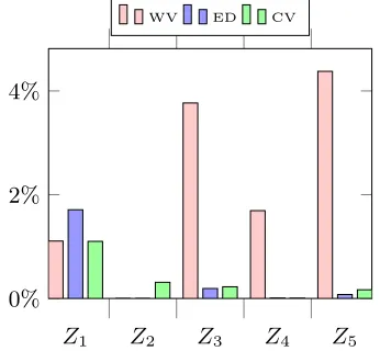
Fig. 4.Dataset VRP-50 – gap to the target.
Figure 3 shows that forZ1 and Z2 the target achievement is close to 100% on all three objective functions. On Z3 the WV objective function noticeably presents the worst results, with only 63% achievement while the ED and CV objective functions both present similar results with near 80% achievement. Fi-nally, on Z4 and Z5 the ED objective function presents a small advantage and the CV objective function is clearly the worst forZ5.
Figure 4 reflects the findings of the previous figure whereZ3shown the lowest overall target achievement. Still, on that objective, the overall gap is below 6% for the three objective functions, hence when the target was not met, the gap still was small. Noticeably, the ED objective function presents the lowest gaps. Moreover, Figure 5 shows that except for WV onZ3, all objective functions on all objectives present improvements over the target solution, noticeably on Z1, Z2 andZ4 where the solutions found are up to 58% better than the target.
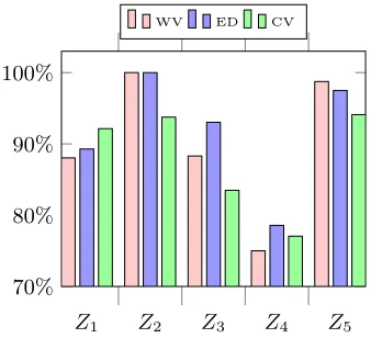
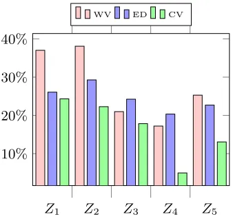
Figures 6–8 present the results for the larger set VRP-150. On figure 6, we see that while on dataset VRP-50 the objective Z3 presents the worst results, in this dataset the worst results appear on Z4 with an average of roughly 75% achievement and, again, the WV objective function presents the worst results. On the other objectives, all objective functions present competitive results.
Figure 7 shows that the gap to the target on solutions that have not met the target is very small – only onZ2the gap is larger than 2% and only for the CV objective function.
Z1 Z2 Z3 Z4 Z5 0%
20% 40% 60%
[image:14.612.224.393.114.271.2]WV ED CV
Fig. 5.Dataset VRP-50 – overall comparison.
Z1 Z2 Z3 Z4 Z5
70% 80% 90% 100%
WV ED CV
Fig. 6.Dataset VRP-150 – target achievement.
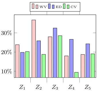
functions, on every objective, the overall quality is more than 20% better than the target. This number increases to nearly 40% for the WV objective function onZ1 andZ2.
Finally, figures 9–11 present the results for the largest dataset VRP-250. Figure 9 presents the target achievement. It can be seen that there is a trend, as the size of the datasets increases, the target achievement of Z1 decreases. In this dataset, the objectivesZ1 andZ4 presents the worst results. Regarding the objective functions, WV presents the best results forZ1. On the remaining objectives, the ED objective function presents the most competitive results.
[image:14.612.224.393.311.465.2]Z1 Z2 Z3 Z4 Z5 0%
1% 2%
[image:15.612.222.393.107.278.2]WV ED CV
Fig. 7.Dataset VRP-150 – gap to the target.
Z1 Z2 Z3 Z4 Z5
10% 20% 30% 40%
WV ED CV
Fig. 8.Dataset VRP-150 – overall comparison.
Lastly, figure 11 shows the overall comparison of solutions with their targets. Again, the results show that all objective functions achieved improved results, with the ED edgingZ3,Z4 andZ5 and the WV edgingZ1andZ2.
7
Discussion
[image:15.612.224.393.310.469.2]Z1 Z2 Z3 Z4 Z5
60% 70% 80% 90% 100%
[image:16.612.224.394.116.268.2]WV ED CV
Fig. 9.Dataset VRP-250 – target achievement.
Z1 Z2 Z3 Z4 Z5
0% 2% 4%
WV ED CV
Fig. 10.Dataset VRP-250 – gap to the target.
this happened in the larger instances. We speculate that a reason for this is that the largest MOVRPTW datasets are not large enough for the multiobjective algorithms to struggle in finding good approximation sets (as it happened in the larger WSRP datasets). Therefore, as the performance gap between single-objective algorithms and multisingle-objective algorithms is considerably smaller in the MOVRPTW problem instances, the difficulties of reaching the target vector becomes more evident.
[image:16.612.221.394.308.468.2]ob-Z1 Z2 Z3 Z4 Z5 10%
20% 30%
[image:17.612.223.394.112.272.2]WV ED CV
Fig. 11.Dataset VRP-250 – overall comparison.
tain approximation sets with fitness landscape closer the fitness landscape of the optimal Pareto front. Also, there is a higher uniformity of the fitness landscapes across instances for these datasets (Pinheiro et al., 2017). All this means that the identified target solutions were realistic, so they could be achieved on every instance. Hence, the CV objective function, which benefits from that, presented good results.
On the MOVRPTW datasets, except for a few exceptions, all objective func-tions were able to not only reach the target but also to substantially improve all objectives – also a reflection of the quality of the approximation set obtained by the multiobjective algorithms.
Nonetheless, it is clear that estimating the Pareto front for problem instances that have similar fitness landscape to the pilot instance, is an effective way to tackle the problem. While the multiobjective algorithms required up to four hours to obtain the approximation set for the pilot instance of a dataset, the GA managed to find competitive solutions in minutes. For the majority of the experiments, targets were achieved and the overall quality of results was high.
8
Conclusion
solutions with goal programming. One is the Chebychev approach that seeks to achieve a solution balanced on all the objective targets. Another one is minimis-ing a weighted function derived from the target solution. The third approach is to use the Euclidean distance to drive the search guided by the target solution. This methodology was first applied by Pinheiro et al. (2018) to real-world instances of a Workforce Scheduling and Routing Problem (WSRP) in the home healthcare sector. In the present paper, the methodology has been further tested by applying it to a different multiobjective problem arising in logistic operational scenarios, the Multiobjective Vehicle Routring Problem with Time Windows (MOVRPTW). In both of these problem scenarios, instances usally arise from different planning periods and hence they present similarities in the fitness land-scapes. This is because usually in this type of real-world problems, instances have the same partial data (e.g. same fleet of vehicles or same set of workers). This paper has shown that the proposed technique is an effective and efficient approach to tackle real-world multiobjective highly-constrained combinatorial optimisation problems, by combining the effectiveness (but often computation-ally expensive) of state-of-the-art multiobjective algorithms with the efficiency of well-targeted single-objective optimisation through goal programming. For this, the multiobjective analysis technique proposed by (Pinheiro et al., 2015, 2017) offers an effective tool to analyse the relationships between objectives in multiobjective optimisation problems and determine the degree of similarity in the fitness landscape of different problem instances.
Azaiez, M. N. and Al Sharif, S. S. (2005). A 0-1 goal programming model for nurse scheduling. Comput. Oper. Res., 32(3):491–507.
Baykasoglu, A. (2005). Preemptive goal programming using simulated annealing.
En-gineering Optimization, 37(1):49–63.
Br¨aysy, O. and Gendreau, M. (2005). Vehicle routing problem with time windows, part ii: Metaheuristics. Transportation Science, 39(1):119–139.
Calvete, H. I., Gal, C., Oliveros, M.-J., and Snchez-Valverde, B. (2007). A goal pro-gramming approach to vehicle routing problems with soft time windows. European
Journal of Operational Research, 177(3):1720 – 1733.
Castro-Gutierrez, J., Landa-Silva, D., and Moreno, P. J. (2011). Nature of real-world multi-objective vehicle routing with evolutionary algorithms. Systems, Man, and
Cybernetics (SMC), 2011 IEEE International Conference on, pages 257–264.
Castro-Gutierrez, J., Landa-Silva, D., and Moreno Perez, J. (2015). Movrptw dataset. https://github.com/psxjpc/. Accessed: 2018-04-24.
Charnes, A. and Cooper, W. (1977). Goal programming and multiple objective opti-mizations. European Journal of Operational Research, 1(1):39 – 54.
Deb, K., Pratap, A., Agarwal, S., and Meyarivan, T. (2002). A fast and elitist multiob-jective genetic algorithm: NSGA-II. Evolutionary Computation, IEEE Transactions on, 6(2):182–197.
Feliot, P., Bect, J., and Vazquez, E. (2016). A bayesian approach to constrained single-and multi-objective optimization. Journal of Global Optimization, pages 1–37.
Flavell, R. B. (1976). A new goal programming formulation. Omega, 4(6):731 – 732.
Ghoseiri, K. and Ghannadpour, S. F. (2010). Multi-objective vehicle routing problem with time windows using goal programming and genetic algorithm. Applied Soft
Computing, 10(4):1096 – 1107.
Giagkiozis, I. and Fleming, P. (2012). Methods for many-objective optimization: An analysis. Research Report No. 1030.
Giagkiozis, I. and Fleming, P. (2014). Pareto front estimation for decision making.
Evolutionary Computation, MIT Press.
Hannan, E. (1980). Nondominance in goal programming.INFOR: Information Systems
and Operational Research, 18(4):300–309.
Jones, D. and Tamiz, M. (2010). Goal Programming Variants, pages 11–22. Springer US, Boston, MA.
Jones, D. and Tamiz, M. (2016). A Review of Goal Programming, pages 903–926. Springer New York, New York, NY.
Leung, S. C. H. (2007). A non-linear goal programming model and solution method for the multi-objective trip distribution problem in transportation engineering.
Op-timization and Engineering, 8(3):277–298.
Mishra, S., Prakash, Tiwari, M. K., and Lashkari, R. S. (2006). A fuzzy goal-programming model of machine-tool selection and operation allocation problem in fms: a quick converging simulated annealing-based approach. International Journal
of Production Research, 44(1):43–76.
Musa, A. A. and Saxena, U. (1984). Scheduling nurses using goal-programming tech-niques. IIE Transactions, 16(3):216–221.
Pinheiro, R. L., Landa-Silva, D., and Atkin, J. (2015). Analysis of objectives relation-ships in multiobjective problems using trade-off region maps. InProceedings of the
2015 Annual Conference on Genetic and Evolutionary Computation, GECCO ’15,
pages 735–742, New York, NY, USA. ACM.
Pinheiro, R. L., Landa-Silva, D., and Atkin, J. (2017). A technique based on trade-off maps to visualise and analyse relationships between objectives in optimisation problems. Journal of Multi-Criteria Decision Analysis, 24(1-2):37–56.
Pinheiro, R. L., Landa-Silva, D., Laesanklang, W., and Constantino, A. A. (2018). Us-ing goal programmUs-ing on estimated pareto fronts to solve multiobjective problems.
InProceedings of the 7th International Conference on Operations Research and
En-terprise Systems - Volume 1: ICORES,, pages 132–143. INSTICC, SciTePress.
Romero, C. (1991). Titles of related interest. InHandbook of Critical Issues in Goal
Programming. Pergamon, Amsterdam.
Tamiz, M., Jones, D. F., and El-Darzi, E. (1995). A review of goal programming and its applications. Annals of Operations Research, 58(1):39–53.
Tamiz, M., Mirrazavi, S., and Jones, D. (1999). Extensions of pareto efficiency analysis to integer goal programming. Omega, 27(2):179 – 188.
Toth, P. and Vigo, D. (2002). The Vehicle Routing Problem. Monographs on Discrete Mathematics and Applications. Society for Industrial and Applied Mathematics.