rspa.royalsocietypublishing.org
Research
Cite this article:Collis J, Brown DL, Hubbard ME, O’Dea RD. 2017 Effective equations governing an active poroelastic medium.Proc. R. Soc. A473: 20160755.
http://dx.doi.org/10.1098/rspa.2016.0755
Received: 6 October 2016 Accepted: 16 January 2017
Subject Areas:
applied mathematics, mathematical modelling, biomechanics
Keywords:
multiscale asymptotics, fluid–structure interaction, poroelasticity, growing media
Author for correspondence: R. D. O’Dea
e-mail:reuben.odea@nottingham.ac.uk
Effective equations governing
an active poroelastic medium
J. Collis, D. L. Brown, M. E. Hubbard and R. D. O’Dea
School of Mathematical Sciences, University of Nottingham,
University Park, Nottingham NG7 2RD, UK
JC,0000-0001-8715-2813; DLB,0000-0002-3421-1063; MEH,0000-0001-7471-1815; RDO,0000-0002-1284-9103
In this work, we consider the spatial homogenization of a coupled transport and fluid–structure interaction model, to the end of deriving a system of effective equations describing the flow, elastic deformation and transport in an active poroelastic medium. The ‘active’ nature of the material results from a morphoelastic response to a chemical stimulant, in which the growth time scale is strongly separated from other elastic time scales. The resulting effective model is broadly relevant to the study of biological tissue growth, geophysical flows (e.g. swelling in coals and clays) and a wide range of industrial applications (e.g. absorbant hygiene products). The key contribution of this work is the derivation of a system of homogenized partial differential equations describing macroscale growth, coupled to transport of solute, that explicitly incorporates details of the structure and dynamics of the microscopic system, and, moreover, admits finite growth and deformation at the pore scale. The resulting macroscale model comprises a Biot-type system, augmented with additional terms pertaining to growth, coupled to an advection–reaction–diffusion equation. The resultant system of effective equations is then compared with other recent models under a selection of appropriate simplifying asymptotic limits.
1. Introduction
Poroelasticity is concerned with the study of elastic bodies that contain pore structures saturated with fluids. The characterization of poroelastic media has garnered much attention over the last 50 years across a wide range of fields studied by applied mathematicians and engineers. Of particular current importance is the study of poroelasticity in biological materials (e.g. in modelling
2
rspa.r
oy
alsociet
ypublishing
.or
g
Proc
.R.
Soc
.A
47
3
:2
0160755
...
solid tumours [1,2] or tissue engineering applications [3]) and the subsurface (e.g. in oil reservoir
engineering, radioactive waste disposal, CO2 sequestration, hydraulic and thermal fracturing,
and cavity generation [4,5]). While there are well-known equations governing poroelasticity at
the so-called macroscopic lengthscale (i.e. a lengthscale much greater than that of the pores)
[6–9], these laws typically requireab initioa statement of the constitutive laws describing the bulk
properties of the solid and fluid components that are averaged volumetrically, irrespective of any underlying structure. As a result, any effective coefficients are meaningful only at the macroscopic scale and models must be parametrized via macroscopic experiments. Given these deficiencies, a model that explicitly accounts for pore-scale physics provides numerous benefits. In general, however, the underlying fluid–structure interaction (FSI) problems are highly complex, multiphysical and nonlinear coupled processes, for which direct simulation on complicated pore structures over multiple lengthscales is practically impossible. As such, effective models that explicitly incorporate pore-scale physics into a macroscopic model provide theoretical and computational benefits at the expense of a mathematically challenging homogenization process. It is beyond the scope of this work to present a comprehensive review and comparison of upscaling techniques that may be employed in the field of poroelasticity. However, in addition to multiscale homogenization, we wish to highlight other applicable techniques such as effective medium
theory [10,11], mixture theory [12–14] and volume averaging [15,16]. For a more complete
discussion we refer the reader to review articles that discuss upscaling in the wider fields of
poroelasticity [17], flow in porous media [18,19] and solute transport [20].
In addition to the classical difficulties associated with poroelastic media, in many applications the solid is ‘active’; that is to say, not only does the solid undergo elastic deformation, but it is also
growing/swelling (or equivalently shrinking)1as a result of some physical, chemical or biological
process. For example, in the context of biological tissue growth, we may view the biological material as a poroelastic medium that is subject to a nutrient-regulated growth law, whereby the mass and volume of the solid material increases over time. For sufficiently large growth rates, this will inevitably affect the macroscopic flow and passive transport of nutrient through the tissue. Similar effects are present in geophysical applications such as swelling in porous clays and coal
[21], as well as in industrial media such as absorbent hygiene products, where electrochemical
processes dominate [21–23]. In this work, we present a general formulation by which a range of
such biologically or industrially motivated problems may be studied. In particular, we consider the derivation of a system of effective macroscopic equations governing a growing poroelastic medium together with passive transport of a solute which acts to regulate the growth dynamics of the medium, by means of two-scale asymptotics. While the techniques employed here may apply naturally to other formulations, here we forgo consideration of other forms of ‘active’ media, such as those that are thermo- or electromechanically active. Moreover, the growth law considered in the current work does not incorporate complex phase transition effects that would provide a more complete description of the underlying systems in the aforementioned applications.
Multiple-scale asymptotics allows the derivation of effective models at the macroscale that explicitly incorporate microstructural information. The application of these techniques is, however, meaningful only for problems in which there are multiple lengthscales that are well separated and there is sufficient uniformity (in the sense of periodicity) in the microscopic
structure; see, for example, [24]. In this framework, local problems are derived that relate
the microscopic and macroscopic structures, which may subsequently be employed in the construction of effective coefficients. The resultant models can be made rigorous via two-scale
convergence, oscillatory test functions, etc. [25,26]. Though this is beyond the scope of this work,
examples employing such methods include computational frameworks such as the multiscale
finite element method [27,28] where the corrector estimates are utilized in error estimation.
A wide range of biological applications employing multiscale methods may be found in the
literature, including [29–34], for example.
3
rspa.r
oy
alsociet
ypublishing
.or
g
Proc
.R.
Soc
.A
47
3
:2
0160755
...
Of particular relevance to this study are [35–37]. In [35], the authors present a rigorous
derivation of the Biot model of poroelasticity [6,7] via multiple-scales expansions. In a recent
work [36], an extension of the analysis in [35] is performed to consider a growing, elastic solid.
The multiscale model in [36] permits finite microscale growth via an accretion growth law, though
it makes the assumption of infinitesimal elastic deformation at the pore scale. Other recent works that consider the multiscale analysis of growing materials are also highly pertinent; see, for
example, [38–40]. In [37], the authors consider the homogenization of an FSI system under finite
pore-scale deformation in a common reference frame. Such an approach has also been applied
successfully in homogenizing domains with evolving microstructure [41–43].
The study of growing material is of great importance in the biological sciences [44,45], and is a
field in which there remain many open mathematical questions. One of the earliest applications of continuum mechanics in the study of growth of deformable biological materials was described in
[46]. Later significant studies in the field include [47,48], which study both volumetric growth and
accretion. However, the key reference in morphoelasticity (i.e. the study of growth in deformable
media) is [49], in which a general formulation for finite volumetric growth in elastic tissues is
proposed. Alternative proposals for growth models may also be found in [50,51]. While much of
the literature pertaining to growth in deformable media is biologically focused, there are many applications in the physical sciences in which solid materials undergo volumetric changes as a result of external drivers such as temperature or the presence of chemical species. In particular, we highlight the similarity between biological growth, swelling in geological media such as clays and shales, and absorbent thin porous media in industrial applications described earlier.
The analysis we present in this work represents a significant extension of classical homogenization techniques of flow and transport in porous media. Here, we extend both the extensive literature pertaining to the homogenization of flow and transport in standard (i.e. not growing) porous media across the physical and biological sciences (see, for example
[26,35,52,53]); and the recent attempts to apply these ideas to growing material in [36,38,39]. These
studies typically place asymptotic restrictions on the underlying model to reduce the degree of
nonlinearity (e.g. the linear coupling between fluid and solid mechanics employed in [36]) and/or
enforce quasi-static conditions (e.g. the movement of the free interface as described in [38,39]). In
this article, we present a framework in which we consider the fully coupled, nonlinear system of equations describing growth, transport and mechanics that results from finite growth and deformation at the pore scale when employing a growth model which neglects effects associated with complex phase transitions. The subsequent application of two-scale asymptotic techniques to this system of equations is further complicated by the fact that the equations governing the fluid and solid mechanics are most naturally written in different reference frames. As such, the system of equations describing the FSI does not yield a coherent understanding of the relationship between microscopic and macroscopic quantities because the periodicity assumption no longer
holds. We proceed following the techniques set out in [37], whereby the FSI problem is written in
a unified periodic domain, to which we apply asymptotic techniques. However, this work further
represents a significant extension of that presented in [37], as here we both consider a hyperelastic
solid material and employ a morphoelastic growth law along similar lines to that described in
[49,54], as opposed to the linearly elastic inactive solid material considered therein.
This article is organized as follows. In §2, we introduce the fine-scale FSI model for the growing deformable medium. In §3, we rewrite all equations in a common periodic reference geometry, derive a system of cell equations at the microscale and effective macroscale equations, and summarize our new formulation. Then, in §4 we demonstrate the relationship between our new model and other recent models by considering appropriate limiting cases. Finally, in §5 we make concluding remarks and highlight ongoing and future work.
2. Model description
4
rspa.r
oy
alsociet
ypublishing
.or
g
Proc
.R.
Soc
.A
47
3
:2
0160755
...
of the growth law we consider, following closely that presented in [49,54], after which we present
the equations governing the fluid motion, elastic deformation and solute transport. For the sake of generality and clarity of presentation, the model presented here is intentionally generic. Biological or physical motivation is therefore minimal, except where necessary for rationalizing specific modelling choices. Given this generality, the analysis and resultant effective equations presented here may prove applicable in many fields of study, though our primary motivations are biological tissue growth and hydrogeology.
Throughout this work, we denote by∇ξ,∇ξ·andξ the gradient, divergence and Laplacian,
respectively, for differentiation with respect to the coordinateξ. For a vector fieldΥ, rank 2 tensor
fieldsAandB, rank 3 tensor fieldA, and rank 4 tensor fieldA, we define
(∇ξΥ)ij=∂Υ∂ξi
j, (∇ξ A)ijk=
∂Aij ∂ξk, (∇ξ
A)ijkl= ∂Aijk
∂ξl and (∇ξ·
A)i= ∂Aij
∂ξj , (2.1)
and the contractions
A:B=AijBij, (A:B)i=AijkBjk and (A :B)ij=AijklBkl, (2.2)
where we employ the Einstein summation convention over repeated indices. Finally, for a scalar
functionψ(A), we define
∂ψ(A)
∂A
ij
=∂ψ(A)
∂Aij . (2.3)
Given the large amount of mathematical notation employed in the remainder of this article, we
have included a brief summary of the nomenclature intable 1, given in appendix A.
(a) Idealized porous medium in the reference configuration
We consider an idealized porous medium in Rd, d=2, 3. We model the medium as a highly
connected material (i.e. both fluid and solid portions of the material are connected) with a (locally) spatially periodic microstructure comprising a growing, hyperelastic solid saturated with a viscous Newtonian fluid. Further, we consider the growth dynamics of the solid to be governed by the availability of a passive solute transported through the domain. We make the assumption that the porous material may be characterized by two distinct lengthscales: the
lengthscale corresponding to the full extent of the material, denoted L and referred to as the
macroscale, and that corresponding to the periodic microstructure, denotedand herein referred
to as the microscale or pore scale. We assume that there is a strong separation of lengthscales;
that is, the dimensionless parameterε=/Lsatisfies 0< ε1. For simplicity in what follows, we
shall scale the macroscopic parameter with unity, i.e.L=1, andε=1.
We denote by Ωε the initial macroscale reference domain, which comprises the periodic
microstructure, and denote the homogenized macroscopic domain byΩ. Throughout this work,
we employ the subscriptεto signify dependence on the material’s microstructure. We further
partition Ωε into two macroscopic subdomains ΩεF and ΩεS such that Ω¯Fε ∪ ¯ΩSε = ¯Ωε and
ΩF
ε ∩ΩεS= ∅; whereΩεF andΩεS correspond to the regions of Ωε containing fluid and solid
material, respectively, and the notation¯denotes the closure of a domain. In addition, we assume
that the fluid domain is sufficiently connected to obtain a non-trivial flow and the solid domain is sufficiently connected to prevent pieces of solid being carried away by the fluid. Furthermore,
we denote byΓεthe initial reference interface betweenΩεF andΩεS. Finally, we denote the unit
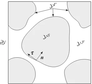
inward normal toΩεSonΓεbynε, and the unit tangent(s) toΓεbyτε.
We specify that the microstructure may be characterized such that the fluid and solid
subdomains may be decomposed into a set of unit cells{YS
5
rspa.r
oy
alsociet
ypublishing
.or
g
Proc
.R.
Soc
.A
47
3
:2
[image:5.493.174.321.40.175.2]0160755
...
YS
YF ∂Y
n
YG
t
Figure 1.Schematic of the reference cell,Y, decomposed into the fluid domainYF, the solid domainYSand the interface YΓ. (Adapted from [39, fig. 1].)
some suitable index setI. Given the periodicity of the microstructure, each cell corresponds to a
translation of a single reference cell; that is,
YiS=YS+ki and YiF=YF+ki, whereki∈Zd∀i∈I. (2.4)
Under this notation we may decompose the solid and fluid domains as
ΩS
ε =
ki:i∈I
ε(YS+ki)∩Ωε and ΩεF= ki:i∈I
ε(YF+ki)∩Ωε. (2.5)
We may further denote the reference cell byY=YS∪YF and denote the fluid–solid interface in
the reference cell byYΓ= ¯YS∩ ¯YF. Moreover, we denote the unit inward normal toYSonYΓby
nand tangents onYΓbyτ. A schematic diagram of the reference cellYis shown infigure 1.
(b) Morphoelastic growth law
We consider finite growth and deformation of the elastic bodyΩεS, employing the theory of solid
mechanics to describe the deformations of the body under the load and stress induced through the growth of the body and its interaction with the surrounding fluid. Following the decomposition
first described in [49] in the field of morphoelasticity, given an initial, residual stress-free reference
configuration the model of growth employed here may be described in two stages:
(i) We consider a geometric (stress-free) deformation of the body which characterizes
the physical/chemical/biological processes governing growth to obtain avirtual grown
configuration.
(ii) We then consider the elastic response of this grown body as a means of enforcing physical compatibility and the physical constraints imposed on the elastic body via its interactions
with the surrounding fluid and geometry to obtain thecurrent deformed configuration.
This second stage is of crucial importance as we make the assumption that the growth process itself is entirely local at each point, that is, independent of the growth nearby. Given such an assumption, it is possible that non-physical configurations may arise as a result of the initial growth stage and, as such, the elastic response is necessary to obtain physically meaningful results.
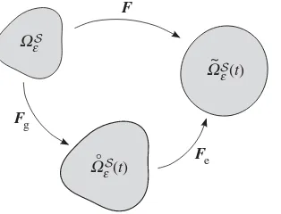
Extending the notation introduced in §2a, we denote the virtual grown configuration byΩ◦Sε
and the current deformed configuration by Ω˜Sε. We now specify that the deformationΩεS→
˜
ΩSε may be characterized by the deformation gradientF. The key tenet of morphoelasticity,
introduced in [49], is that F may be decomposed into the composition of a tensor describing
6
rspa.r
oy
alsociet
ypublishing
.or
g
Proc
.R.
Soc
.A
47
3
:2
[image:6.493.173.330.43.163.2]0160755
...
F
Fe Fg
W°e (t)
W~e (t) W e
Figure 2.Schematic diagram of the decomposition into the growth and elastic response deformations. WhereF,FgandFe
denote the total, growth and elastic deformations andΩε,Ω◦ε(t) andΩ˜ε(t) denote the initial reference, virtual grown and current deformed configurations, respectively.
diagram demonstrating the decomposition of the deformation and the notation for the variously
transformed domains is given infigure 2. This approach has been adopted widely in the field
of biomedical engineering and we refer to the review articles [55,56] for discussion regarding its
application. We highlight, for example, the application to cardiac [57], arterial [45] and skin [58]
tissue growth models, and the comparisons against relevant clinical/experimental data therein, in particular.
While, conceptually, this decomposition appears natural, there is a subtlety in its application to time-dependent continuous growth, which we discuss briefly, following closely the exposition
given in [54]. In growth mechanics, there are typically four time scales of interest: corresponding
to elastic wave propagation (τe), viscoelastic relaxation (τv), external loading (τl) and growth (τg).
Implicit in the above is the assumption that the decomposition is instantaneous, insomuch as it
applies continuously in time and, asFgevolves,Feresponds instantaneously. This requires strong
separation between the growth time scale and the elastic time scales. In the following analysis, we neglect elastic wave propogation and viscoelastic effects and, as such, make no further reference
toτeandτv,2and concentrate solely on effects occurring on time scalesτlandτgin the remainder
of this article. While there may be regimes in which growth time scales become comparable to others, we assume here that growth time scales are larger than the other pertinent time scale with
τlτg, (2.6)
as in [54]. Under this ordering of the time scales, elastic responses of the material occur much
quicker than growth, so that for time smaller thanτgthe solid material is in a quasi-static elastic
equilibrium. As such, we consider that the only pertinent time variation is that associated with the evolution of the growth tensor given by
dFg
dt =H(Fe,Fg,. . .;t). (2.7)
We now consider a time incrementδt, such thatτlδtτg, and apply a single time step of a
forward Euler method to (2.7) to obtain
Fg(t+δt)=Fg(t)+δtH(Fe,Fg,. . .;t). (2.8)
This permits the definition of an incremental growth and elastic deformation associated withδt
by
Finc=Fince ◦Fincg , (2.9)
where Fincg :=δtH. In the following, we consider only incremental growth deformation
gradients and as such forgo the notation associated with incremental growth for presentational
7
rspa.r
oy
alsociet
ypublishing
.or
g
Proc
.R.
Soc
.A
47
3
:2
0160755
...
reference configuration
t = t0 t = t1 t = t2 t = tn
Fg, 1 Fg, 2 Fg, 3 Fg,n
Fe,n
Fe, 1 Fe, 2
current configurations with growth and elastic responses stress-free grown states
W e W° W°e(t2)
e (t1) W
°
e(tn)
W~e(tn)
W~e(t1) W
~
e(t2)
W~e(t1) W
~
e(t2) W
~
e(ttn)
Figure 3.Schematic diagram of the decomposition into the growth and elastic response deformations for multiple incremental growth steps, whereFg,iandFe,idenote the growth and elastic deformations to
◦
Ωε(ti) andΩ˜ε(ti), respectively, associated with
transition from timeti−1toti.
convenience. The above definition of incremental growth and response provides a natural means of considering many growth steps. A schematic diagram demonstrating the application of
multiple growth steps is given in figure 3. In the multiple-scales analysis presented in §3, we
consider a single time increment only for the sake of concision, though we remark that the homogenization process generalizes naturally to any number of time steps.
As a means of modelling either nutrient-regulated growth in biological applications or chemical-regulated degradation in industrial applications, we additionally specify that the
growth is coupled to transport. Under this assumption, Fg has a functional dependence on
the concentration of solute, denotedcε. For simplicity, we setFg=Fg(cε) and do not consider
explicit stress or time dependencies on growth. Additionally, we consider the transport of solute
on the diffusive time scale τD. Whether there is a strong separation between τg and τD is
application specific and, therefore, in the following analysis we make no assumptions regarding the separation between these two scales. Further restrictions on the constitutive assumption for the underlying growth law are described in §2f.
In order for us to specify correctly the equations governing fluid and solid mechanics, and transport of the passive solute, we must define appropriate coordinate systems in the reference, virtual grown and deformed current configurations. As such, consider the mappings
◦
χε(t) :Ωε→Ω◦ε(t) and χ˜ε(t) :Ω◦ε(t)→ ˜Ωε(t), (2.10)
wherebyχ◦εis obtained by appropriate constitutive assumptions on the growth dynamics, and
˜
χεis obtained via solution of an elasticity problem. Under these definitions, a pointPinΩεwith
coordinatesxat timethas coordinatesx◦=χ◦ε(x,t) inΩ◦ε(t) andx˜= ˜χε(x◦,t) inΩ˜ε(t). Moreover, we
may naturally define the grown and deformed full domains, fluid domains and interface by ◦
Ωε(t)= {χ◦
ε(x,t) :x∈Ωε}, Ω˜ε(t)= { ˜χε◦χ◦
ε(x,t) :x∈Ωε},
◦
ΩFε(t)= {χ◦ε(x,t) :x∈ΩεF}, Ω˜Fε(t)= { ˜χε◦χ◦ε(x,t) :x∈ΩεF}, ◦
Γε(t)= {χ◦ε(x,t) :x∈Γε}, Γ˜ε(t)= { ˜χε◦χ◦ε(x,t) :x∈Γε}.
For clarity, in the following we further identify all dependent variables defined with respect to the
8
rspa.r
oy
alsociet
ypublishing
.or
g
Proc
.R.
Soc
.A
47
3
:2
0160755
...
we remark that we defer explicit definition of the deformationsχ◦εandχ˜εuntil the definition of
the constitutive assumption on the equations governing the elastic deformation in §2d and the growth law given in §2f.
(c) Fluid equations
The motion of the fluid is governed by the incompressible Navier–Stokes equations; however,
following the arguments presented in [38,39,59] we assume that the microstructure and fluid
velocity are scaled such that the time derivative and inertial terms in the Navier–Stokes equations
are O(ε2). Further, we note that these equations are most naturally presented in the current
deformed configuration. Denoting the pressure, velocity and dynamic viscosity of the fluid by
˜
pε,v˜εandμ, respectively, the fluid inΩ˜Fε(t) is governed by the Stokes equations
−∇x˜p˜ε+μ∇x˜·(∇x˜v˜ε+(∇˜xv˜ε)T)= ˜fεF ∀˜x∈ ˜ΩFε(t) (2.11)
and
∇x˜· ˜vε=0 ∀˜x∈ ˜ΩFε(t), (2.12)
where f˜Fε denotes an external force acting on the fluid. We note that, while the momentum
equation (2.11) is quasi-steady,p˜εandv˜εhave implicit time dependence due to the growth and
mechanics of the solid material.
It remains for us to specify the conditions governing the flow on the interface Γ˜ε and the
remainder of the boundary∂Ω˜ε. As this requires coupling with the solid equations (which are
described in the grown domain) and periodicity (which is applicable only in the initial reference configuration), we defer their specification until §2g, once appropriate coordinate transformations have been defined.
(d) Solid equations
We assume that the solid material is hyperelastic, i.e. the constitutive assumption on its stress may be determined via an appropriate strain energy functional. We proceed now by specifying the equations governing the deformation of the solid, presented in the current grown configuration
(see [60,61]). Recalling the notation introduced in §2b, we define the elastic deformation
gradient by
Fe:= ∇◦
xχ˜ε, (2.13)
and the right Cauchy–Green deformation tensor by
Ce:=FTeFe. (2.14)
In view of the time-scale separation (2.6), the solid skeleton satisfies
− ∇◦
x· ◦
σεS=f◦Sε ∀x◦∈Ω◦Sε, (2.15)
wheref◦Sε denotes a body force acting on the solid material andσ◦Sε denotes the Piola stress in the
body. As we consider a hyperelastic material, we defineσ◦Sε constitutively by
◦
σSε :=2Fe∂Ψ( Ce)
∂Ce , (2.16)
whereΨ(Ce) denotes the strain energy functional for a given material. In the analysis presented
in §3b(ii), we require that the strain energy functional satisfies certain convexity requirements and, as such, we restrict our attention to materials whose strain energy functionals are strictly
polyconvex (for a definition see, for example, [61]) such as Ogden [62] or Mooney–Rivlin [63,64]
9
rspa.r
oy
alsociet
ypublishing
.or
g
Proc
.R.
Soc
.A
47
3
:2
0160755
...
more, we defer the specification of suitable interface and boundary conditions to §2g, after the definition of relevant coordinate transformation tensors.
(e) Solute transport
In addition to considering the motion of the fluid and solid materials, we further model the
transport of a passive solute whose concentration we denotecε. As we consider growth regulated
by the passive solute, the evolutions of the fluid and solid domains are coupled tocεas well as to
each other through the FSI. In the fluid and solid domains (Ω˜Fε andΩ˜Sε, respectively), we assume
that the solute is transported via advection and diffusion (in the latter, the advection arising due to the growth and deformation of the solid material). In the solid, however, we consider an additional consumption term associated with growth. Finally, we note that the equations governing the transport of this solute in each sub-domain are most naturally posed in the current deformed configuration as diffusive fluxes are associated with spatial concentration gradients, as opposed to material gradients in the grown or initial configurations.
Given these assumptions, the equations governing the evolution of this transported species in
˜
ΩFε is given by
∂˜cε
∂t + ∇˜x·(v˜ε˜cε)=DFx˜c˜ε ∀˜x∈ ˜ΩFε, (2.17)
whereDFdenotes the diffusivity of the solute in the fluid; and the evolution inΩ˜Sε is given by
∂c˜ε
∂t + ∇x˜·
∂χ˜
∂tc˜ε
=DSx˜˜cε−RS˜cε ∀˜x∈ ˜ΩSε, (2.18)
whereDSdenotes the diffusivity of the solute andRSis a constant that denotes the consumption
of solute in the solid material. We note that in generalRSmay have a complicated dependence
on a range of model variables which we neglect here for the sake of clarity of presentation.
(f) Assumption on the growth law
We now specify assumptions on growth that we employ in the following analysis. For the sake of simplicity, we consider that the growth of the solid material is isotropic and a function of the local concentration of solute only. Under these assumptions, the natural form of the growth displacement is given by
◦
χε(x)=χ◦ε(x,cε), (2.19)
in which there is an implicit time dependence provided by the coupling to cε(x,t). The
deformation gradient associated with the growth deformation is then given by
Fg:= ∇xχ◦ε(x,cε). (2.20)
We note that for simplicity, and as we wish to maintain a general formulation in this study, the growth law employed here does not incorporate complicated phase transitions and stress dependence that are often employed in the modelling of biological materials. We refer the reader
to, for example, [56] for further discussion on growth laws in a biological setting. In particular,
we highlight the lack of non-local terms corresponding to consumption of the fluid phase that may occur in certain applications described previously under the assumption of a more complex growth law.
(g) Interface conditions
10
rspa.r
oy
alsociet
ypublishing
.or
g
Proc
.R.
Soc
.A
47
3
:2
0160755
...
Recalling the definition ofnε, we define the trace of a scalar quantityψ (defined inΩεF andΩεS),
onΓεby
ψ±:=lim
→0ψ(x±nε). (2.21)
Under this notation, we define the jump operator by
[[ψ]]=ψ+−ψ−, (2.22)
where we extend to vector and tensor quantities componentwise according to this definition.
(i) Fluid–structure coupling
The natural conditions to impose in the current context of FSI are continuity of velocity and continuity of total stress. However, a complication lies in the fact that the fluid and solid equations
are presented with respect to different configurations (i.e.Ω◦ε(t) andΩ˜ε(t), respectively). We must
therefore consider appropriate transformations of the fluid stress, in view of which we defer the definition of the interface conditions to §3a, wherein we describe the process of mapping the FSI problem to a unified periodic domain.
(ii) Solute
Suitable conditions for the concentration of the passive solute are continuity of solute concentration and flux across the interface, i.e.
[[D∇x˜c˜ε· ˜nε(t)]]=0 ∀˜x∈ ˜Γε (2.23)
and
[[c˜ε]]=0 ∀˜x∈ ˜Γε. (2.24)
As in the case of the fluid–structure coupling, we will subsequently be required to map these conditions onto the interface in the initial reference configuration when we come to perform the multiple-scale asymptotic analysis.
3. Homogenization in the Lagrangian frame
In this section, we describe the process of mapping the system of equations describing the FSI in §2c,d, and the solute transport in §2e, to a periodic reference geometry on which we may perform the two-scale asymptotic analysis. We then proceed by applying two-scale expansions and spatially averaging to obtain cell problems on the microscale (i.e. problems posed on the
periodic cellY), and effective equations in the homogenized macroscale domainΩ.
(a) Coordinate transformations
In this section, we apply a coordinate transformation to the equations governing the FSI and solute transport, together with the appropriate interface conditions, to yield a full system of
equations on the fixed reference configuration denoted Ωε. This process is analogous to the
so-called arbitrary Lagrangian–Eulerian (ALE) formulation widely employed in computational
studies; see [37,65].
Recalling from §2d,f the definitions ofFeandFg, we observe that these tensors are well defined
11
rspa.r
oy
alsociet
ypublishing
.or
g
Proc
.R.
Soc
.A
47
3
:2
0160755
...
their definition to all ofΩ◦εby means of a suitable harmonic extension. We now define the Piola
transformations,Gα, and Jacobians,Jα, by
Jα=detFα and Gα=JαF−1α forα∈ {e,g}. (3.1)
Following [65], we are able to obtain the identities for the transformation of derivatives under a
generic mapping. Consider a general mappingχˇεdefined by
ˇ
χε:Ωˆε→ ˇΩε
and xˆ→ ˇx.
(3.2)
We denote the associated gradient of the mapping byF#= ∇xˆχˇε, and defineG#andJ#according
to (3.1). Then, denoting a generic scalar fieldξ, vector fieldΥ and tensor fieldA, and adopting
the convention of usingˆandˇto denote evaluation inΩˆεandΩˇε, respectively, application of the
chain rule yields
∇xˇξˇ=F−#T∇xˆξˆ and ∇xˇΥˇ =(∇xˆΥˆ)F−1# . (3.3)
Via the application of Nanson’s formula and the divergence theorem, we obtain
∇xˇ· ˇΥ= 1
J#∇xˆ·(J#
F−1# Υˆ) and ∇xˇ· ˇA= 1
J#∇xˆ·(J#
ˆ
AF−#T). (3.4)
Lastly, the chain rule provides
∂ξˇ ∂t =
∂ξˆ ∂t −
F−1# ∂χˇε
∂t · ∇xˆ
ˆ
ξ. (3.5)
By substituting the appropriate nomenclature associated with the mappingsχ◦ε andχ˜εinto
(3.3)–(3.5), we are able to obtain expressions for mapping derivatives between the reference, virtual grown and current deformed configurations.
We now proceed to write the coupled FSI, growth and transport problem in the initial reference configuration employing (3.3)–(3.5). The first stage of this process is to rewrite these equations in the virtual grown configuration, thus obtaining a system equivalent to that obtained in the ALE
frame in [37]. The second stage, which differentiates this work from [37], is to further map the
equations obtained in the grown configuration,Ω◦ε, to the periodic reference configurationΩε. To
this end, and for the sake of concision, we introduce the following notation corresponding to the combination of growth and elastic deformation:
F:=FgFe, G:=GgGe and J:=JgJe. (3.6)
The equations governing the fluid are thus given by
−GT∇xpε+μ∇x·((∇xvε)GF−T+GT(∇xvε)TF−T)=JfFε ∀x∈ΩεF (3.7)
and
∇x·(Gvε)=0 ∀x∈ΩεF. (3.8)
The equations governing the elastic deformation are given by
− ∇x·(σSεGTg)=JgfSε ∀x∈ΩεS. (3.9)
The equations governing the transport in the fluid domain are
J
∂cε
∂t −2
F−1g ∂ ◦ χε
∂t · ∇x
cε
+ ∇x·(cεGvε)=DF∇x·(GF−T∇xcε) ∀x∈ΩεF, (3.10)
and in the solid domain
J
∂cε
∂t −
F−1g ∂
◦ χε
∂t · ∇x
cε
+ ∇x·
JF−1g ∂ ◦ χε
∂t
cε
12
rspa.r
oy
alsociet
ypublishing
.or
g
Proc
.R.
Soc
.A
47
3
:2
0160755
...
We note that, despite the elastic deformation affecting transport, the time derivative of the elastic deformation does not appear in (3.11) explicitly due to our choice of temporal scalings. The coupling of the fluid and solid problems is specified via the velocity condition
vε=gε ∀x∈Γε, (3.12)
wheregεdenotes the interfacial growth velocity defined by
gε:=Fe∂ ◦ χε
∂t , (3.13)
and the stress condition
σFεGTnε=σSεGTgnε ∀x∈Γε, (3.14)
whereσFε is the fluid stress, defined by
σF
ε := −pεI+μ((∇xvε)F−1+F−T(∇xvε)T). (3.15)
Finally, the coupling between the concentration of solute is given by
[[cε]]=0 and [[D∇xcε·nε]]=0 ∀x∈Γε. (3.16)
(b) Multiscale homogenization
We now analyse the coupled system describing the FSI, growth and transport of the passive solute in the fixed reference configuration derived in §3a, with the aim of obtaining a macroscopic
description in a manner analogous to that presented in [35–37]. Given the structure of the medium
introduced in §2, we naturally define
y:=1
εx (3.17)
to be the spatial coordinate associated with the microscale (or fast moving coordinate), where
x now corresponds to the spatial coordinate associated with the macroscale (or slow moving
coordinate). Under the assumption of strong separation of scales, we may expand each dependent
variableψin multiple-scales form via an expansion
ψ(x,y,t;ε)=
∞
i=0
εiψ(i)(x,y,t). (3.18)
Moreover, under this coordinate transformation the gradient operator∇xis transformed as
∇x→ ∇x+1
ε∇y, (3.19)
where∇x and∇y denote differentiation with respect to the macroscale and microscale spatial
variables, respectively. We proceed by writing expansions of the form (3.18) for the dependent
variablescε,χ˜εandpε. Following [24,35–37], we then assume a standard scaling for Stokes flow
and expandvεaccording to
vε(x,y,t;ε)=ε2
∞
i=0
εiv(i)(x,y,t), (3.20)
and in order to maintain the correct scaling we follow [37,59] and scale the interfacial growth
velocity employed in (3.12) with
gε=ε2g. (3.21)
We emphasize that this scaling ensures that growth and flow are of equal importance, rather than a simplifying relegation to lower order as commonly employed elsewhere. In particular, it implies that, while growth is finite, it is slow, consistent with (3.20).
As in [37], we expandFe,JeandGeaccording to (3.18), and we further propose the expansion
ofFg,JgandGgin a similar manner. We note that in §3b(i) we are required to assume that the
13
rspa.r
oy
alsociet
ypublishing
.or
g
Proc
.R.
Soc
.A
47
3
:2
0160755
...
subsequently show, in §3b(ii), that under the assumption of strict polyconvexity of the strain energy functional this assumption is indeed valid and independent of the analysis presented in
§3b(i). We constitutively specifyFg=Fg(cε) and subsequently show (see §3b(iii)) that at leading
order the solute concentration exhibits no microscale dependence (as is typical of similar models
[38,39]). Correspondingly, we may reasonably assume that χ◦ε is sufficiently smooth that the
growth deformation gradient may be expanded as
Fg=F(0)g (x)+εFg(1)(x,y)+O(ε2), (3.22)
where such an assumption permits the following analysis. Following this, we may expand the Jacobian for the growth deformation as
Jg=Jg(0)(x)+εJg(1)(x,y)+O(ε2)
=det(F(0)g (x))+εJ(1)g (x,y)+O(ε2). (3.23)
We note that it is straightforward to obtain expressions forJ(1)g in terms of the components ofFg;
however, a precise expression for this term is not required for the analysis that follows and so is
omitted for concision. For a generic tensorA, under the assumption thatεis sufficiently small
that
−∞
i=1
εiA(i)(A(0))−1 op
<1,
we may obtain, by application of a Neumann series, the following expansion for its inverse,A−1,
A−1= ∞
j=0
−∞
i=1
εiA(i)(A(0))−1 j
(A(0))−1
=(A(0))−1−εA(1)(A(0))−2+. . .
=
i=0
εi(A−1)(i). (3.24)
Given this observation, we note that we may write the Piola transformation associated with growth as
Gg=G(0)g (x)+εG(1)g (x,y)+O(ε2)
=det(F(0)g (x))(F(0)g (x))−1+εG(1)g (x,y)+O(ε2). (3.25)
As above, an explicit expression forG(1)g is straightforward to obtain but is not included.
Remark 3.1. While we consider here a growth law that is dependent on the concentration of a solute, the following analysis naturally generalizes to a growth law that is dependent on any quantity that is microscale invariant to leading order.
Finally, we substitute each of these expansions, together with (3.19), into the system of
equations set out in §3a to obtain a system of PDEs at increasing orders ofε.
To obtain the homogenized macroscale equations in the following sections, we take spatial averages of leading-order behaviour. To this end, we define the following integral averages associated with the reference cell:
ψYF= 1
|Y|
YF
ψdy, ψYS= 1
|Y|
YS
ψdy and ψYΓ= 1
|Y|
YΓ
ψds, (3.26)
and the material porosity,φ, by
φ=|YF|
14
rspa.r
oy
alsociet
ypublishing
.or
g
Proc
.R.
Soc
.A
47
3
:2
0160755
...
(i) Fluid flow
We now consider the equations governing the fluid flow inYFobtained at increasing orders ofε.
AtO(ε−1) the equations are given by
(G(0))T∇yp(0)=0 (3.28)
and
∇y·(G(0)v(0))=0. (3.29)
From (3.28), we observe thatp(0)is locally constant inYF, i.e.p(0)=p(0)(x,t). AtO(1), we obtain
the momentum equation
−(G(0))T(∇xp(0)+ ∇yp(1))+μ∇y·D(0)(v(0))=J(0)fFε, (3.30)
whereD(n)(·) denotes a modified rate of strain tensor defined by
D(n)(Υ) :=((∇yΥ)G(n)(F(n))−T+(G(n))T(∇yΥ)T(F(n))−T). (3.31)
Equations (3.30) and (3.29) now provide the so-called cell problem inYF for the fluid.3As such,
we propose the following ansatz for the leading-order velocity and first-order pressure: v(0)=W
1∇xp(0)+W2fFε (3.32)
and
p(1)=π1· ∇xp(0)+π2·fFε, (3.33)
where Wi and πi (i=1, 2) are rank 2 tensors and vectors, respectively, that satisfy a pair of
modified tensor Stokes problems, given by
−(G(0))T∇yπ1+μ∇y·D(0)(W1)=(G(0))T ∀y∈YF,
∇y·(G(0)W1)=0 ∀y∈YF ⎫ ⎬
⎭ (3.34)
and
−(G(0))T∇yπ2+μ∇y·D(0)(W2)=J(0)I ∀y∈YF,
∇y·(G(0)W2)=0 ∀y∈YF, ⎫ ⎬
⎭ (3.35)
whereWiandπiarey-periodic,Wi=0onYΓ andπiare mean-free onYFfori=1, 2.
The conservation of fluid mass atO(1) is given by
∇x·(G(0)v(0))+ ∇y·(G(1)v(0)+G(0)v(1))=0. (3.36)
To obtain the macroscopic equation governing the fluid, we substitute the ansätze given in (3.32)
and (3.33) into the conservation of fluid mass equation given at O(1) and average over the
reference cell. Application of the divergence theorem andy-periodicity then yields
∇x·(G(0)v(0)YF)+ (G(1)v(0)+G(0)v(1))·nYΓ=0. (3.37)
On a further application of the divergence theorem (this time onYS) and the substitution of the
velocity interface condition given in (3.12), we obtain
∇x·(G(0)v(0)YF)+ ∇y·(G(1)g(0)+G(0)g(1))YS=0. (3.38)
Finally, substituting in the ansatz forv(0)and the definitions ofg(0)andg(1)we obtain
∇x·(K∗∇xp(0)+J∗fF)+g∗100+g∗010+g∗001=0 (3.39)
inΩ, where
K∗:= G(0)W1YF, J∗:= G(0)W2YF, g∗ijk:=
∇y· ⎛ ⎝G(i)F(ej)∂
◦ χ(k)
∂t ⎞ ⎠
YS
. (3.40)
15
rspa.r
oy
alsociet
ypublishing
.or
g
Proc
.R.
Soc
.A
47
3
:2
0160755
...
Note that in (3.39) and (3.40) we are required to computeF(1)e andG(1), and that these quantities
depend on∇yχ˜(2)and∇yχ◦
(2)
, and hence the system is not closed. Therefore, we are required to
make appropriate closure assumptions. Here, we consider first order only correctors forχ˜ andχ◦
in the definition ofF(1)e andG(1), i.e. we replace these tensors in (3.39) and (3.40) with
ˆ
F(1)e := ˆF(1)e (χ˜(0),χ˜(1)) and Gˆ(1):= ˆG(1)(χ˜(0),χ˜(1),χ◦
(0)
,χ◦(1),c(0),c(1)). (3.41)
We note that the validity of such closure assumptions will depend on the constitutive assumptions and parameter values employed in specific scientific and engineering applications. As such, we do not comment here on the domain of their applicability, but rather highlight this for consideration in future computational studies.
(ii) Elastic deformation
A corresponding macroscale description for the elasticity equations, parametrized by suitable microscale cell problems, is obtained by an almost identical process to that outlined in §3b(i) (see
also [66] and the references cited therein). First, we define the Piola stress in the initial reference
geometry by
Te:=σSεGTg. (3.42)
We now propose the expansion of the Piola stress of the form
Te= ∞
i=−1
εiT(i)
e, (3.43)
which may be obtained by considering expansions forGgand∂Ψ(Ce)/∂Ceat increasing orders
ofε. We note that this expansion runs fromi= −1 as there is a spatial derivative implicit in the
definition ofσSε. AtO(ε−2) in (3.9), we obtain
− ∇y·(T(−1)e (χ˜(0),c(0)))=0 ∀y∈YS. (3.44)
AsF(0)g andG(0)g exhibit noy-dependence and we have restricted our choice of material such that
the strain energy functional is strictly polyconvex, the resultant strong ellipticity of the operator
[61] yields that the leading-order elastic deformation exhibits no microscale dependence (see
[66–68] and associated literature discussingΓ-convergence [69–71]). From this observation, we
deduce thatT(−1)e ≡0and that the proposed expansions forFe,JeandGeemployed in [37] are
also correct here.
Collecting terms atO(ε−1), we obtain
− ∇y·(T(0)e (χ˜(1),χ˜(0),c(0)))=0 ∀y∈YS. (3.45)
The coupling between the fluid and solid domains is given by the stress interface condition (3.14), from which we obtain
T(0)e (χ˜(1),χ˜(0),c(0))n= −p(0)(G(0))Tn ∀y∈YΓ. (3.46)
Analogously to (3.32) and (3.33), we now propose the following ansatz for the first-order displacement:
˜
χ(1)=N(x,y) :∇
xχ˜(0), (3.47)
whereNis a rank 3 tensor that satisfies the cell problem
− ∇y·(T(0)e (N;χ˜(0),c(0)))=0 ∀y∈YS, (3.48)
subject toy-periodicity and the interface condition
16
rspa.r
oy
alsociet
ypublishing
.or
g
Proc
.R.
Soc
.A
47
3
:2
0160755
...
Here, we consider (3.48) and (3.49) as the equations governingN, which is nonlinearly coupled to
the macroscale quantitiesp(0),∇xu(0)andc(0)via the implicit dependence of the stress onF(0)g and
G(0)g . In (3.48) and (3.49), all microscale derivatives∇yact onN only (both through divergence
and the definition ofFe, and henceCe). As such, we adopt the notationT(0)e (N;·) to clarify that
this problem determinesN, parametrized by the quantities appearing after the semi-colon that
vary on the macroscale only.
AtO(1), we then obtain
− ∇y·T(1)e − ∇x·(T(0)e (χ˜(1),χ˜(0),c(0)))=J(0)g fSε. (3.50)
Substituting in the ansatz (3.47) and taking they-average overYSwe obtain
− ∇y·T(1)e YS− ∇x·(T(0)e (χ˜(0);N,c(0))YS)=J(0)g fSε, (3.51)
where we now viewT(0)e as a function ofχ˜(0), parametrized byN andc(0). Focusing on the first
term in (3.51) and utilizing the divergence theorem, we obtain
−∇y·T(1)e YS= − 1
|Y|
YΓT (1) e nds
=|1
Y|
YΓ(σ
F
εGT)(1)nds
= ∇y·((σFεGT)(1))YF. (3.52)
In view of (3.52), and rewriting the fluid stress in terms of fluid pressure and velocity via (3.15) (and exploiting the ansätze (3.32) and (3.33)), we obtain the general homogenized equation governing solid mechanics given by
− ∇x· T(0)e (χ˜(0);N,c(0))YS=Jg(0)fSε −(M1∗−α∗1I)∇xp(0)−(M2∗−α∗2I)fFε +β∗p(0) (3.53)
inΩ, where
M∗i =μ∇y·((∇yWi)G(0)(F(0))−T+(G(0))T(∇yWi)(F(0))−T)YF
and α∗i = ∇y·((G(0))Tπi)YF, β∗= ∇y·(G(1))TYF.
⎫ ⎬
⎭ (3.54)
(iii) Solute transport
In this section, we consider the homogenization of the solute transport equations ((3.10) and (3.11)) in the periodic reference configuration. We proceed as in §3b(i),(ii) to obtain the equation
governing the transport of solute atO(ε−2)
D∇y·(G(0)(F(0))−T∇yc(0))=0 (3.55)
throughoutY, where we define
D=
DS inYS
DF inYF. (3.56)
The interface condition atO(ε−1) is given by
[[c(0)]]=0 and [[D∇yc(0)·n]]=0. (3.57)
Under the assumption of periodicity of F(0)e , F(0)g , G(0)e and G(0)g , we conclude that c(0) is
17
rspa.r
oy
alsociet
ypublishing
.or
g
Proc
.R.
Soc
.A
47
3
:2
0160755
...
CollectingO(ε−1) terms, we obtain
D∇y·(G(0)(F(0))−T(∇xc(0)+ ∇yc(1)))=0 ∀y∈YF (3.58)
and
D∇y·(G(0)(F(0))−T(∇xc(0)+ ∇yc(1)))= ∇y·
J(0)(F(0)g )−1∂χ˜
(0)
∂t
c(0) ∀y∈YS, (3.59)
subject to the interface conditions atO(1)
[[c(1)]]=0 and [[D(∇xc(0)+ ∇yc(1))·n]]=0. (3.60)
We propose the following ansatz forc(1):
c(1)=Q· ∇xc(0). (3.61)
Substituting (3.61) into (3.58)–(3.60), we obtain the cell problems forQgiven by
D∇y·(G(0)(F(0))−T(I+(∇yQ)T))=0 ∀y∈YF (3.62)
and
D∇y·(G(0)(F(0))−T(I+(∇yQ)T))=fQ ∀y∈YS, (3.63)
subject to the interface conditions
[[Q]]=0 and [[D(I+(∇yQ)T)n]]=0 ∀y∈YΓ (3.64)
andy-periodicity overY, where the additional forcing in (3.63),fQ, is given by
fQ:=
⎧ ⎪ ⎪ ⎨ ⎪ ⎪ ⎩
∇y·(J(0)(F(0)g )−1(∂χ˜(0)/∂t))c(0) d
i=1(∂c(0)/∂xi)
1 ifc(0)=0,
0 ifc(0)=0,
(3.65)
where 1 denotes a vector of length d whose entries are all 1. Collecting terms at O(1),
substituting in the ansatz (3.61) and averaging over the reference cellY, we obtain the macroscale
homogenized PDE governing the leading-order concentration of the solutec(0), given by
J(0)Y∂c
(0)
∂t −V∗· ∇xc(0)= ∇x·D∗∇xc(0)+R∗c(0) (3.66)
inΩ, where we define the effective advective velocity associated with growth by
V∗=(1+φ)(F(0)g )−1
J(0)(I+(∇yQ)T)∂ ◦ χ(0)
∂t
Y
, (3.67)
the effective diffusivity by
D∗=DG(0)(F(0))−T(I+(∇yQ)T)Y, (3.68)
and the effective reaction by
R∗=(φ−1)
⎛ ⎝RSJ(0)
YS+
∇y·
JF−1g ∂ ◦ χ
∂t (1)
YS ⎞
⎠. (3.69)