The data analysis pipeline for the SDSS IV MaNGA IFU Galaxy Survey : overview

The Data Analysis Pipeline for the SDSS-IV MaNGA IFU Galaxy Survey: Overview

Kyle B. Westfall,1 Michele Cappellari,2 Matthew A. Bershady,3, 4 Kevin Bundy,1Francesco Belfiore,5, 1 Xihan Ji,6 David R. Law,7 Adam Schaefer,3 Shravan Shetty,3 Christy A. Tremonti,3 Renbin Yan,8

Brett H. Andrews,9 Joel R. Brownstein,10 Brian Cherinka,11, 7 Lodovico Coccato,12 Niv Drory,13

Claudia Maraston,14 Taniya Parikh,14 Jos´e R. S´anchez-Gallego,15Daniel Thomas,14 Anne-Marie Weijmans,16

Jorge Barrera-Ballesteros,11 Cheng Du,6 Daniel Goddard,14 Niu Li,6Karen Masters,17

H´ector Javier Ibarra Medel,18 Sebasti´an F. S´anchez,18 Meng Yang,16 Zheng Zheng,19, 20 andShuang Zhou6

1_{University of California Observatories, University of California, Santa Cruz, 1156 High St., Santa Cruz, CA 95064, USA} 2_{Sub-department of Astrophysics, Department of Physics, University of Oxford, Denys Wilkinson Building, Keble Road, Oxford OX1}

3RH, UK

3_{Department of Astronomy, University of Wisconsin-Madison, 475N. Charter St., Madison WI 53703, USA} 4_{South African Astronomical Observatory, P.O. Box 9, Observatory 7935, Cape Town, South Africa} 5_{European Southern Observatory, Karl-Schwarzchild-Str. 2, Garching bei M¨unchen, 85748, Germany} 6_{Tsinghua Center of Astrophysics & Department of Physics, Tsinghua University, Beijing 100084, China}

7_{Space Telescope Science Institute, 3700 San Martin Drive, Baltimore, MD 21218, USA}

8_{Department of Physics and Astronomy, University of Kentucky, 505 Rose Street, Lexington, KY 40506, USA} 9_{University of Pittsburgh, PITT PACC, Department of Physics and Astronomy, Pittsburgh, PA 15260, USA} 10_{University of Utah, Department of Physics and Astronomy, 115 S. 1400 E., Salt Lake City, UT 84112, USA}

11_{Center for Astrophysical Sciences, Department of Physics and Astronomy, Johns Hopkins University, 3400 North Charles Street,} Baltimore, MD 21218, USA

12_{European Southern Observatory, Karl-Schwarzchild-str., 2, Garching b. M¨unchen, 85748, Germany} 13_{McDonald Observatory, The University of Texas at Austin, 1 University Station, Austin, TX 78712, USA} 14_{Institute of Cosmology & Gravitation, University of Portsmouth, Dennis Sciama Building, Portsmouth, PO1 3FX, UK}

15_{Department of Astronomy, University of Washington, Box 351580, Seattle, WA 98195, USA} 16_{School of Physics and Astronomy, University of St Andrews, North Haugh, St Andrews KY16 9SS, UK}

17_{Department of Physics and Astronomy, Haverford College, 370 Lancaster Ave, Haverford, PA 19041} 18_{Instituto de Astronoma, Universidad Nacional Aut´onoma de M´exico, A.P. 70-264, 04510, Mexico, D.F., M´exico}

19_{National Astronomical Observatories of China, Chinese Academy of Sciences, 20A Datun Road, Chaoyang District, Beijing 100012,} China

20_{CAS Key Laboratory of FAST, NAOC, Chinese Academy of Sciences}

(Received; Revised; Accepted)

Submitted to AJ

ABSTRACT

Mapping Nearby Galaxies at Apache Point Observatory (MaNGA) is acquiring integral-field spec-troscopy for the largest sample of galaxies to date. By 2020, the MaNGA Survey — one of three core programs in the fourth-generation Sloan Digital Sky Survey (SDSS-IV) — will have observed a statistically representative sample of 104_{galaxies in the local Universe (z}

.0.15). In addition to a ro-bust data-reduction pipeline (DRP), MaNGA has developed a data-analysis pipeline (DAP) that provides higher-level data products. To accompany the first public release of its code base and data products, we provide an overview of the MaNGA DAP, including its software design, workflow, measurement procedures and algorithms, performance, and output data model. In conjunction with our companion paper Belfiore et al., we also assess the DAP output provided for 4718 observations of 4648 unique galaxies in the recent SDSS Data Release 15 (DR15). These analysis products focus on measurements that are close to the data and require minimal model-based assumptions. Namely, we provide stellar kinematics (velocity and velocity dispersion), emission-line properties (kinematics, fluxes, and equiv-alent widths), and spectral indices (e.g., D4000 and the Lick indices). We find that the DAPprovides

Corresponding author: Kyle B. Westfall westfall@ucolick.org

robust measurements and errors for the vast majority (>99%) of analyzed spectra. We summarize assessments of the precision and accuracy of our measurements as a function of signal-to-noise, and provide specific guidance to users regarding the limitations of the data. The MaNGADAPsoftware is publicly available and we encourage community involvement in its development.

Keywords: methods: data analysis – techniques: imaging spectroscopy – surveys – galaxies: general – galaxies: fundamental parameters

1. INTRODUCTION

Publicly available data sets in accessible formats play an increasingly important role in astronomy, broadening access and enabling analyses that combine observations across wavelengths and telescopes. The original Sloan Digital Sky Survey (SDSS, York et al. 2000) initiated an ongoing commitment to publicly release raw and re-duced data that continues through the current genera-tion, SDSS-IV (Blanton et al. 2017).

With the introduction of the MaNGA Survey (Map-ping Nearby Galaxies at Apache Point Observatory,

Bundy et al. 2015), SDSS-IV data releases have included “higher dimensional” sets of datacubes whose produc-tion requires a sophisticated Data Reducproduc-tion Pipeline (Law et al. 2016,DRP). Over its six-year duration ending July 2020, MaNGA is providing spatially resolved spec-troscopy for 10,000 nearby galaxies selected withM∗& 109_M

and hzi ∼ 0.03 (Wake et al. 2017). MaNGA uses specially designed fiber bundles (Drory et al. 2015) that feed the BOSS spectrographs (Smee et al. 2013) on the 2.5-meter Sloan Telescope (Gunn et al. 2006). Span-ning 0.36–1.0µmat a resolution of R∼2000 and with excellent flux calibration (Yan et al. 2016a), MaNGA executes approximately three-hour long dithered inte-grations (Law et al. 2015) to reach signal-to-noise re-quirements for galaxies observed to approximately 1.5 effective (half-light) radii, Re, (two-thirds of the sam-ple) and 2.5 Re (one-third of the sample) (Yan et al.

2016b).

Reduced MaNGA data, including reconstructed dat-acubes, are produced by the automated MaNGA DRP

and have been made publicly available since the thir-teenth SDSS data release (DR13;Albareti et al. 2017). Inspired by previous “value-added catalogs” (VACs) based on SDSS data, with the MPA-JHU1 _{catalog for}

SDSS-I/II being a prime example, members of the MaNGA team have also provided publicly available VACs in previous data releases.2

The complexity and richness of spatially-resolved data sets, like those produced by MaNGA, as well as the de-sire to take on common analysis tasks that would oth-erwise be duplicated by large numbers of users has

mo-1 _{https://www.sdss.org/dr15/data access/} value-added-catalogs/mpa-jhu-stellar-masses

2 _{For example: https://www.sdss.org/dr14/data access/} value-added-catalogs/

tivated SDSS-IV to invest in a “project-led” MaNGA Data Analysis Pipeline (DAP). By providing a uniform set of commonly desired analysis products, theDAPalso enables rapid and interactive delivery methods for these data products, helping scientists quickly design samples of interest and make discoveries. It was also appreciated that while researchers would likely perform custom mea-surements of primary interest to their science, the ability to combine these with readily available DAP measure-ments that might otherwise be outside their expertise would open up new opportunities. In general, a broad-based and robustDAPmakes MaNGA data more science-ready. This strategy aligns with other IFU surveys in-cluding ATLAS3D3 _{(Cappellari et al. 2011), CALIFA}4

(S´anchez et al. 2012), and SAMI5 (Croom et al. 2012) that have released high-level data products.

The MaNGA DAP has been under development since 2014, evolving through several versions and a transition from an original IDL to python implementation. Al-though theDAPhas primarily been used as a survey-level pipeline for providing analysis products to the SDSS col-laboration, our development strategy has also empha-sized flexibility to prospective users. The low-level, core algorithms have been constructed in a way that is largely independent of their specific use with the MaNGA data, allowing a user to write newpythonscripts aroundDAP

functions or classes for analysis of more varied data sets. Additionally, the high-level interface is written such that the detailed execution of many of the internal algorithms can be modified using a set of configuration files, allow-ing a user to tailor how theDAPanalyses MaNGA data to better suit their scientific needs. Although much of the high-level functionality assumes one is working with MaNGA data, it is possible to apply the DAP to data from different instruments with modest modification.

The MaNGA science teams have published studies based on DAP output throughout its development, us-ing internal data releases to the SDSS collaboration that we term MaNGA Product Launches (MPLs). TheDAP

source code continues to evolve as we improve its fidelity and expand its functionality. We encourage community involvement in these efforts via our public repository on

GitHub.6 _{The GitHub repository also contains some}

example scripts that use low-level DAPfunctions to fit a single spectrum, as well as the higher-level modules (Section 4) that can be used to fit a single datacube. Additional example scripts will be provided as develop-ment continues, and we encourage others to submit their own scripts via a GitHub pull request.

This paper describes the first public release of DAP

products, as part of SDSS Data Release 15 (DR15), and includes both the code (version2.2.1) and output data products. The public DAPoutput is available for down-load from the SDSS website7_{and viaMarvin}8_(Cherinka et al. 2019) — an interactive web-based interface to both MaNGA datacubes andDAPquantities (Marvin-Web), as well as apython package (Marvin-tools) that enables seamless remote and/or local access to these MaNGA data that can be incorporated in anypython-based anal-ysis workflow.

The primary output of theDAPincludes stellar kine-matics, fluxes and kinematics of emission lines, and continuum spectral indices. In deriving these mea-surements, the DAP makes heavy use of pPXF ( Cappel-lari & Emsellem 2004;Cappellari 2017) as a workhorse spectral-fitting routine. Our philosophy has been to focus on measurements that are made directly on the MaNGA spectra and that do not require significant model-based assumptions. For example, the DAP fits stellar template mixes plus a polynomial component to the stellar continuum. This provides an excellent rep-resentation of the data and derived stellar absorption-line kinematics, but is not necessarily appropriate for accurate stellar-population properties. For maps of es-timated stellar age, metallicity, star-formation histo-ries, and other model-derived data products, the Fire-fly (Goddard et al. 2017) and Pipe3D (S´anchez et al. 2016a,b) VACs9 _{are valuable resources. Pipe3D}

prod-ucts in particular also include alternative measurements of kinematics and emission lines.

In this contribution, we present an overview of the MaNGA DAP, its algorithmic structure, and its output data products. We begin in Section 2 with a “quick-start” guide that provides a more detailed introduction to the DAPoutput and nomenclature by way of exam-ples. Along with many other resources cited therein, we expect Section 2 to be a useful road map to the DAP

products and the rest of our paper. In Section 3, we describe the input data required by the DAP, including a general summary of MaNGA spectroscopy. Section 4

provides an overview of theDAPworkflow through its six main analysis modules. After first describing the

spec-6 _{https://github.com/sdss/mangadap} 7 _{https://www.sdss.org/dr15/data access} 8_{https://dr15.sdss.org/marvin}

9 _{https://www.sdss.org/dr15/data access/} value-added-catalogs/

tral templates we use in DR15 and the method used to generate them in Section 5, we dedicate the following five sections to the detailed description of each of the

DAPanalysis modules:10

Section 6 describes our spatial binning approach and the importance of including spatial covariance in these calculations. Section7 goes into particular depth with regard to the assessments of the stellar kinematics. We present results from several input/output simulations, as well as a statistical comparison of the results for MaNGA galaxies with multiple observations. In particular, these repeat observations allow us to provide a detailed assess-ment of the errors reported by theDAP. We use Section

8 to introduce our bandpass-integral formalism that is used when measuring both non-parameteric emission-line fluxes and spectral indices. Section9describes our emission-line modeling algorithm, with detailed assess-ments of the module and usage in DR15 provided by our companion paper, Belfiore et al. accepted. Finally, Section10describes our quantification of continuum fea-tures using spectral indices, and we assess the accuracy and precision of our measurements using a similar ap-proach used for the stellar kinematics. Detailed quality assessments of the two full-spectrum-fitting modules are provided in Section 7 (stellar kinematics) and Belfiore et al., accepted, (emission-line modeling), and we com-ment on the overall performance of theDAPfor DR15 in Section11. In particular, we note specific regimes where we find theDAPcurrently requires further development. Section12provides a detailed discussion of theDAP out-put products and important aspects of these products that users should keep in mind. Finally, we provide some brief conclusions in Section13. AppendicesA,B, andC

provide, respectively, theDAPprocedure used to match the spectral resolution of two spectra, an assessment of how instrumental resolution errors propagate to errors in the stellar velocity dispersion measurements, and ta-bles describing theDAPoutput data models.

Unless stated otherwise, throughout this paper: (1) We adopt a ΛCDM cosmology with Ωm= 0.3, ΩΛ= 0.7, andH0= 100hkm s−1 Mpc−1. (2) All wavelengths are provided in vacuum. (3) All flux densities have units of 10−17 ergs/cm2/s/˚A/spaxel.

2. DAPQUICK-START GUIDE

We begin with a “quick-start guide” to the MaNGA

DAP, jumping right into example output products that highlight key aspects of the DAPmeasurements. To be clear from the beginning,all of the DAPinput and out-put files we discuss here and throughout our paper are

(b) S/Ng

2

4

10

20 (c) V

100

50

0

50

100 (d)

10

20

40

100 (e) Vgas

100

50

0

50

100 (f) H

10

20

40

100

(g) H EW

4

10

20 (h) H Flux

0.1

1

(i) H Flux

0.1

1

(j) [OIII] Flux

0.1

1

(k) [NII] Flux

0.1

1

(l) [SII] Flux

0.1

1

10 0 10 20 10 0 10 (m)

[a

rc

se

c]

[arcsec]

D4000

1.5

1.6

1.7

1.8 (n) H A

1

2

3

4

5

6 _{(o) H}

2.5

3.0

3.5

4.0

4.5 (p) Mgb

1.5

2.0

2.5

3.0

3.5 (q) Fe

1.5

2.0

2.5

3.0 (r) NaD

1

2

3

Figure 1. A subset of the DAP-derived quantities for datacube 8439-12703, the observation of MaNGA galaxy 1-605884

(z = 0.025; log(M∗/h−2M) = 10.2;Re= 1100.8∼4.2 h−1 kpc; seehttps://sas.sdss.org/marvin/galaxy/8439-12703/for more information about this galaxy and its properties in the larger context of the MaNGA sample.) From top-to-bottom and left-to-right: (a) the SDSSgricomposite image with the nominal size of the IFU outlined in purple; (b) theg-band S/N per channel, S/Ng; (c) the stellar line-of-sight (LOS) velocity,V∗; (d) the stellar velocity dispersion,σ∗; (e) the ionized-gas LOS velocity,Vgas;

(f) the velocity dispersion of the Hαemission line,σHα; (g) the equivalent width (EW) of the Hαemission line; (h) the flux of the Hαemission line; (i) the flux of the Hβemission line; (j) the total flux in the [OIII]λ4959,5007 emission lines; (k) the total flux in the [NII]λ6548,6583 emission lines; (l) the total flux in the [SII]λ6716,6730 emission lines; (m) the D4000 spectral index; (n) the HδA spectral index; (o) the Mgb spectral index; (q) the average of the Fe5270 and Fe5335 spectral indices,hFei; (r) and the NaD spectral index. The gray circle in the bottom-left corner of panels b through r is the nominal FWHM of MaNGA’s spatial resolution element (beam size; 200.5). Bins or spaxels with S/Ng<10 are masked in panel d (σ∗); S/Ng<3 are masked in panel m (D4000); S/Ng<5 are masked for the plotted absorption-line indices (panels n through r); and Hαfluxes less than 2.5×10−18_erg/s/cm2 _{are masked in panel f (σ}

Hα). included as part of DR15. The narrative of this Section aims to help the reader quickly get a sense of those prod-ucts and navigate their way to subsequent sections of our paper that are most relevant to their goals. Although some general guidance can be sufficiently provided here, other more nuanced advice requires the backdrop of our assessments of theDAPdata, performed throughout our paper. In Section 2.1, we highlight specific sections where the reader can go for that advice, as well as other documentation provided as part of SDSS DR15. Finally, Section2.2provides a list of known issues with the DAP

data provided with DR15 that users should take into account.

In Figure1, we show the SDSSgricomposite image for the galaxy targeted by integral-field unit (IFU)12703on plate8439and a sampling of the quantities produced by the DAP for this datacube.11 From top to bottom and

11 _{The python code used to produce this plot and many others} in this paper can be found athttps://github.com/sdss/mangadap/ tree/master/docs/papers/Overview/scripts.

left to right, these images roughly follow the order of the DAP workflow (Section 4), from assessments of the g-band signal-to-noise (S/Ngper spectral pixel; panel b; Section6); to the measurements of the stellar kinematics (panels c and d; Section7); to the emission-line model-ing that produces fluxes, equivalent-widths (EWs), and kinematics (panels e through l; Section 9; Belfiore et al.accepted); and finally to the spectral-index measure-ments (panels m through r; Section10).

The images, or maps, plotted in Figure1are provided by the primaryDAPoutput file, a multi-extension fits file called the MAPS file (Section12.1). TheMAPS files pro-vide each DAP measurement in a two-dimensional im-age format, or map, that exactly matches the spatial dimensions of the DRP datacubes. Where appropriate, each mapped quantity has associated inverse-variance and quality-assessment measurements. Our quality as-sessments are provided by a set of bitmasks defined in Appendix C, and their use is a critical aspect of any workflow incorporating theDAPoutput data. In Figure

field-of-view or because they do not meet the DAP quality-assurance criteria (Section 6.1). For Figure 1 specifi-cally, we also mask regions in the maps of the stellar velocity dispersion (σ∗), Hα velocity dispersion (σHα), and spectral indices at low S/Ng and low flux; see the Figure caption.12 _{A user-customized set ofDAPmaps are}

easily displayed for a specific galaxy inMarvin, both via the web interface13_{and its core}

pythonpackage.14

The DAP results for 8439-12703 (the datacube for galaxy 1-605884) were chosen at random for Figure 1

and are representative of the DR15 results as a whole.15

Using these data as an example, it is important to note that the spatial pixel, or spaxel, size (0.005×0.005) is sig-nificantly smaller than the full-width at half maximum (FWHM) of the on-sky point-spread function (2.005 di-ameter) shown as a gray circle in the bottom-left corner of each panel. This spaxel sampling was chosen as a compromise between the covariance introduced in the datacubes by our reconstruction approach and the spa-tial scale needed to properly sample the dithered fiber observations (cf. Liu et al. 2019). Even so, the subsam-pling of the fiber beam leads to significant covariance between adjacent spaxels (Section6.2; Law et al. 2016) and a few noteworthy implications. First, accounting for this covariance is critical to accurately meeting a tar-get S/N threshold when spatially binning the datacubes (Section6.3). Second, spatial variations in the mapped measurements driven by random errors in the observed spectra should be smooth on scales of roughly 5×5 spax-els. That is, significant spaxel-to-spaxel variations due to a random sampling are highly improbable given the well-defined correlation matrix of the datacube. Instead, a useful rule of thumb to keep in mind when inspecting

DAPimages is that significant spaxel-to-spaxel variations are driven by systematic error,16_{not astrophysical}

struc-ture. On the other hand, structure on scales similar to the beam size could be astrophysical — such as the in-creased HαEW along the spiral arms of galaxy 1-605884 — or driven by noise in the fiber observations — such as is likely the cause of the strong, beam-size variations

12 _{Masking in theDAPis largely limited to indicating numerical} or computational issues occurring during the course of the anal-ysis. Flagging of any given measurement based on its expected quality is more limited due to the difficulty of defining criteria that are generally robust and not overly conservative.

13 _{https://dr15.sdss.org/marvin} 14 _{https://github.com/sdss/marvin}

15 _{Because the same galaxy may be observed more than once} (see Table1), we generally refer to a specific datacube using its PLATEIFUdesignation throughout this paper (e.g.,8439-12703in this case), as opposed to the unique MaNGA ID associated with each survey target.

16 _{The systematic error involved may only yield an increased} stochasticity in the measurements that average out over many spaxels, and does not necessarily imply a systematic shift of the posterior distribution away from the true value.

in the gas velocity field toward the IFU periphery or the high-frequency modulations of its spectral-index maps.

The maps shown in Figure 1 are the result of a “hy-brid” binning approach (see the introduction to Section

9and the algorithm description in Section 9.2). In this approach, the stellar kinematics are measured for spa-tially binned spectra that meet a minimum of S/Ng&10 (Section 6.3) and the emission-line and spectral-index measurements are performed for individual spaxels. We expect these results to be preferable for the majority of users, providing the benefits of both unbiased stellar kinematics and unbinned emission-line maps. The selec-tion of these products is made via the DAPTYPE, as we define below.

A core design principle of theDAPhas been to abstract and modularize the analysis steps to maintain flexibil-ity. The specific combination of the settings used for all analysis steps — e.g., the specific binning algorithm and the templates used to measure the stellar kinematics — adopted for the survey-level execution of the DAPis used to construct a unique keyword called theDAPTYPE; see Section 4 and Figure 3 for more detail. For DR15, two unique approaches to the analysis were performed, meaning that each galaxy datacube is analyzed twice and users must choose which set of products to use (see Section12).17 The fundamental difference between these twoDAPTYPEs is whether the output is based on the hybrid binning approach — the output we recommend users start with — or ifallanalyses have been performed using spectra Voronoi-binned to a target S/Ng&10.

To minimize the complexity of the output DAP data model, measurements made on binned spectra are mapped to each spaxel in the bin. This can be seen in the maps of the stellar kinematics shown in Figure

1, where regions of constant stellar velocity are the vi-sual result of all the relevant spaxels being binned into a single spectrum during the fitting process. Alterna-tively, the remaining maps all show quantities varying spaxel-to-spaxel. If the maps in Figure 1 were instead from the analysis that only used the Voronoi-binned spectra (not the hybrid approach),allmaps would show identical regions of constant values. Although they are convenient for visual inspection and for the simplicity of the data model, it is important to identify and select only the unique measurements for detailed analysis (see other data-model-specific advice in Section12).

Inevitably, visual inspection of theDAPmaps will lead one to find features that are physically counter-intuitive

17 _{For reference, the execution time of the}

4000 5000 6000 7000 8000 9000 1

10 100

8256-9102 Center

Flux Density

[OII]

[NeIII]

H H H

HeII

H

[OIII] HeI

[OI]

H

[NII] [SII]

50 5

/

0 2 4 6 8

Flux Density

8728-12703 Center

CN Fe H Mgb Fe NaD TiO2

H

CaHK aTiO CaH NaI CaII Pa

4000 5000 6000 7000 8000 9000

50 5

/

Rest Wavelength (Å in vacuum)

Figure 2. The central spaxel of datacubes8256-9102(top) and8728-12703(bottom) and the best-fittingDAPmodel spectra.

Flux densities are plotted in units of 10−17 erg/s/cm2/˚A/spaxel. In both panels, the observed spectrum is shown in black, the best-fitting model spectrum (stellar continuum plus emission lines) is shown in red, and the stellar-continuum-only model is shown in blue. The fit residuals are shown directly for 8728-12703, and also shown in separate panels for both spectra after normalizing by the spectral errors, ∆/. The gray region atλ &7340 ˚A is not included in any full-spectrum fit as the stellar spectral templates used for DR15 have no coverage at these wavelengths. The 22 emission lines fit in DR15 (Table 3) are labeled and marked in the top panel by vertical lines colored according to the groups identified in Section 5.3 of Belfiore et al., accepted. The primary passbands of the 43 absorption-line indices measured in DR15 (Table4) are shown against the 8728-12703spectrum: Hydrogen bands are marked in blue; C, N, Ca, or Mg bands are in orange; Fe bands are in green; and Na or TiO bands are in purple. A few bands are labeled according to their name or the element present in their name.

and/or erroneous; we discuss some of these cases in Sec-tion 11.2.2. When in doubt about features seen in the

DAPmaps, there is no substitute for directly inspecting the MaNGA spectral data (Section3;Law et al. 2016) and the associated DAP model spectra. The latter are provided by the second main DAPoutput file, a multi-extension fits file called the model LOGCUBE file (Sec-tion 12.2). This file contains all the model spectra fit to the observations, or provides the information needed to reconstruct the models (see point 2 in Section 12.2). Our Marvin software package and web-based interface (Cherinka et al. 2019) provide particularly useful tools for this kind of data inspection.

Figure 2 shows two high-S/Ng spectra and the best-fittingDAPmodel spectra. Note that the full model (stel-lar continuum and emission lines) is shown in red with the stellar-continuum-only model overlaid in blue; ex-cept for the emission features, therefore, the two are identical such that the model appears blue in most of the Figure. The model spectra are the result of the two full-spectrum fits in the DAP, both of which use pPXF. The first fit masks the emission lines and determines the best fit to the stellar continuum to measure the stellar kinematics (Section 7). The second fit simultaneously optimizes the stellar continuum and emission lines while keeping the stellar kinematics fixed to the result from the first fit (Section 9). The stellar continuum is

han-dled differently between these two fits and yield slightly different results; the continuum shown in Figure2is the result of the combined fit of the second full-spectrum fit (cf. Belfiore et al.,accepted, Figure 2).

Note that the wavelength range fit by the DAP full-spectrum-fitting modules is limited to 0.36–0.74µmfor DR15 because of the spectral range of the templates used (Section5). This has two primary effects. First, it limits the spectral range over which we can fit emission lines. Most notably this excludes modeling of the near-infrared [S III] lines. For this purpose, in particular, we aim to soon take advantage of our in-house stellar li-brary, MaStar18_{(Yan et al. 2018), so that our continuum}

models are fit over MaNGA’s full spectral range. Sec-ond, while we can measure spectral indices at all wave-lengths, we can only calculate the velocity-dispersion corrections (Section10.1) for those measurements in re-gions with valid model fits. This means any spectral index provided in DR15 with a main passband centered at λ > 0.74µm does not include a velocity-dispersion correction, which can be critical when, e.g., analyzing absorption-line strengths as a function of galaxy mass.

The two galaxy spectra in Figure 2 were selected to illustrate the features fit by theDAP. The central spaxel

of datacube 8256-9102 for the star-forming galaxy 1-255959 has extremely bright nebular emission with nearly all 22 emission lines measured in DR15 (Sections

9 and 8; Table 3) identifiable by eye. Indeed, many more emission lines are visible that are not currently fit by the DAP, largely from H and He recombination and N, O, S, and Ar forbidden transitions. We expect to add to the list of lines included in the fit in future re-leases of theDAP, both by extending the spectral range of the continuum models (cf. Belfiore et al. accepted) and controlling for any problems caused by attempting to fit what are generally much weaker lines. The central spaxel of datacube8728-12703of the early-type galaxy 1-51949 has relatively weak emission features but ex-hibits many of the absorption features measured by the 46 spectral indices provided in DR15 (Section 10 and Table4).

2.1. Usage Guidance

Anyone planning to use the DAP data is strongly encouraged to read Section 12. There we describe the main output files provided by the DAP and we highlight a number of aspects of the data important to their use. Some of these are simple practicali-ties of the data model, but others are critical to the proper interpretation of the data. Basic introduc-tions and usage advice for the DAP data products are also included in the DR15 paper (Aguado et al. 2019) and data-release website, https://www.sdss.org/dr15/. From the latter, note the following in particular: an introduction to working with MaNGA data (https: //www.sdss.org/dr15/manga/getting-started/) and some of the intricacies involved (https://www.sdss.org/ dr15/manga/manga-data/working-with-manga-data/), worked tutorials (https://www.sdss.org/dr15/manga/ manga-tutorials/, a list of known problems and caveats (https://www.sdss.org/dr15/manga/manga-caveats/), and the general SDSS helpdesk (https://www.sdss.org/ dr15/help/).

In terms of its general success in fitting MaNGA spec-tra, Section11provides a useful reference if one encoun-ters a missing DAPproduct or a counter-intuitive mea-surement. In particular, Section 11.2.2 provides a list of regimes where fit-quality metrics have been used to identify aberrantly poor spectral fits produced by the

DAP.

Guidance for each of the three primary DAP prod-uct groups (stellar kinematics, emission-line properties, and continuum spectral indices) are provided in, respec-tively, Section7, Belfiore et al.,accepted, and Section10. For thestellar kinematics, we particularly recommend Section 7.7, which provides guidance for how to use our stellar velocity dispersion measurements. For the

emission-line measurements, we recommend that

users read Sections 6 and 7 of Belfiore et al., accepted, at least, and then follow-up with other Sections of their paper as relevant. Finally, for thespectral indices, we

recommend users read the summary of the assessments we have performed herein, provided in Section10.3.4.

2.2. Known Issues in DR15DAPProducts

For general reference, below we provide a list of known issues with the DR15 version of the DAP software and theDAP-derived data products. Where relevant, we pro-vide references to subsequent Sections of our paper with more information; see alsohttps://www.sdss.org/dr15/ manga/manga-caveats/. More up-to-date information and documentation of source code changes are included in the source-code distribution, seehttps://github.com/ sdss/mangadap/blob/master/CHANGES.md.

1. Detailed assessments of the uncertainties provided for the non-parametric emission-line measure-ments have not been performed, meaning their accuracy is not well characterized. We expect they are of similar quality to the spectral-index uncer-tainties (Section 10.3.2); however, they should be treated with caution.

2. Some Milky Way foreground stars that fall within MaNGA galaxy bundles have not been properly masked. More generally, the DAP does not cor-rectly handle the presence of multiple objects in the IFU bundle field-of-view (Section11.2.2).

3. The wings of particularly strong or broad emis-sion lines will not have been properly masked dur-ing the stellar-continuum fits used to measure the stellar kinematics (Section 7.1.2).

4. The MASK extension in the model LOGCUBE files cannot be used to reconstruct the exact mask re-sulting from the stellar-kinematics module.

5. The χ2_ν measurements reported for the stellar-kinematics module are not correct; they do not exclude pixels that were rejected during the fit it-erations.

6. The highest order Balmer line fit by theDAPis Hθ, even though many galaxies show higher-order lines (Figure2).

7. Measurements for the Hζ Balmer line are unreli-able given its blending with the nearby He I line (as reported by Belfiore et al.,accepted).

8. The velocity-dispersion measurements for the [O II] line are improperly masked (also reported by Belfiore et al.,accepted).

10. Velocity dispersion corrections for index measure-ments will include velocity effects because all mea-surements are done using the single bulk redshift to offset the band definitions (Section 10).

3. DAPINPUTS

3.1. MaNGA Spectroscopy

Drory et al. (2015) provide a detailed description of the MaNGA fiber-feed system, which is composed of 17 integral-field units (IFUs): two 19-fiber IFUs, four 37-fiber IFUs, four 61-37-fiber IFUs, two 91-37-fiber IFUs, and five 127-fiber IFUs. The plate scale of the 2.5-meter Sloan telescope yields an on-sky fiber diameter of 200. The combination of the seeing conditions at Apache Point Observatory (APO), the dithering pattern of the MaNGA observational strategy (Law et al. 2015), and the method used to construct the datacubes typically provides a spatial point-spread function (PSF) with a FWHM of∼2.005 (Law et al. 2016). All of the IFUs have their fibers packed in a hexagonal, regular grid with a field-of-view (FOV) directly related to the number of fibers. Including the fiber cladding, the nominal FOV diameters are 1200, 1700, 2200, 2700, and 3200 for the 19-, 37-, 61-, 91-, and 127-fiber IFUs, respectively.

The MaNGA fiber-feed systems are coupled to the SDSS-III/BOSS spectrographs (Smee et al. 2013), a pair of spectrographs with “blue” and “red” cameras that receive, respectively, reflected (λ_.0.63µm) and trans-mitted (λ_&0.59µm) light from a dichroic beamsplitter. The full spectral range obtained for each fiber spectrum is 0.36µm_.λ_.1.03µm after combining the data from both cameras. Each arm of each spectrograph uses a volume-phase holographic grism yielding spectral reso-lutions of Rλ = λ/∆λ ≈ 2000 at λ = 0.55µm for the two blue cameras and Rλ≈2500 at λ= 0.9µm for the two red cameras (seeYan et al. 2016b, Figure 20).

Following the observational strategy outlined byLaw et al. (2015), each MaNGA plate is observed using a three-point dither pattern to fill the IFU interstitial re-gions and optimize the uniformity of the FOV sampling for all 17 targeted galaxies on a plate. Depending on the observing conditions, 2–3 hours of total observing time is required to reach the survey-level constraints on the signal-to-noise (S/N) ratio, as defined byYan et al.

(2016b).

These data are reduced by the MaNGADRP, an IDL -based software package, yielding wavelength-, flux-, and astrometrically calibrated spectra. The reduction pro-cedures are similar to those used by the SDSS-III/BOSS pipeline,19 but with significant adjustments as required by the MaNGA observations. The DRPis described in detail byLaw et al.(2016), the spectrophotometric cal-ibration technique is described by Yan et al. (2016a),

19 _{https://www.sdss.org/dr15/spectro/pipeline/}

and relevant updates to these procedures for DR15 are discussed byAguado et al.(2019).

The spectra from all four cameras are combined into a single spectrum for each fiber resampled to a common wavelength grid. Spectra are produced with both linear and log-linear wavelength sampling. All spectra for a givenPLATEIFUdesignation are included in a single file as a set of row-stacked spectra (RSS) and as a uniformly sampled datacube (CUBE). The MaNGA datacubes are constructed by regridding the flux in each wavelength channel to an on-sky pixel (spaxel) sampling of 0.005 on a side following the method ofShepard(1968); seeLaw et al. (2016, Section 9) for details (cf. S´anchez et al. 2012;Liu et al. 2019). The interpolating kernel is a two-dimensional Gaussian with a standard deviation of 0.007 and a truncation radius of 1.006. Although this interpola-tion process leads to significant covariance between the spaxels in a given wavelength channel (Law et al. 2016, Section 9.3), the currentDAPrelease is primarily focused on working with these resampled datacubes. Also, the

DAPcurrently only analyzes the spectra that are sampled with a log-linear step in wavelength of ∆ logλ= 10−4 (corresponding to a velocity scale of ∆V = 69 km s−1_).

3.2. Photometric Metadata

For convenience, the DAP uses measurements of the ellipticity ( = 1 −b/a) and position angle (φ0) of the r-band surface-brightness distribution to calculate the semi-major-axis elliptical polar coordinates, R and θ, where the radius is provided in arcseconds as well as in units of the effective (half-light) radius, Re. In the limit of a tilted thin disk, these are the in-plane disk radius and azimuth. Except for some targets from MaNGA’s ancillary programs, the photometric data are taken from the parent targeting catalog described by

Wake et al.(2017, Section 2). This catalog is an exten-sion of the NASA-Sloan Atlas (NSA)20 _{toward higher}

redshift (z _.0.15) and includes an elliptical Petrosian analysis of the surface-brightness distributions. Despite this difference with respect to the NSA catalog provided by the catalog website, we hereafter simply refer to this extended catalog as the NSA. The primary advantage of the NSA is its reprocessing of the SDSS imaging data to improve the sky-background subtraction and to limit the “shredding” of nearby galaxies into multiple sources (Blanton et al. 2011).

4. WORKFLOW

At the survey level, theDAPis executed once perDRP

datacube (PLATEIFU). The DAPwill attempt to analyze any datacube produced by theDRP, as long as it is an ob-servation of a galaxy target that has an initial estimate of its redshift. Specifically, we only analyze observations selected from theDRPallfile (Law et al. 2016) for

DAPpython object Analysis objectives MAPS extensions Model

LOGCUBE extensions

ReductionAssessment

SpatiallyBinnedSpectra

StellarContinuumModel

EmissionLineModel

SpectralIndices

SPX_SKYCOO SPX_ELLCOO SPX_MFLUX SPX_SNR

BINID

BIN_LWSKYCOO BIN_LWELLCOO BIN_AREA BIN_MFLUX


BIN_SNR

STELLAR_VEL STELLAR_SIGMA STELLAR_SIGMACORR STELLAR_CONT_FRESID STELLAR_CONT_RCHI2

EMLINE_GFLUX EMLINE_GEW EMLINE_GVEL EMLINE_GSIGMA EMLINE_INSTSIGMA EMLINE_TPLSIGMA

SPECINDEX SPECINDEX_CORR

BINID FLUX IVAR WAVE REDCORR

MODEL EMLINE EMLINE_BASE EMLINE_MASK

• On-sky coordinates • Signal-to-noise • Spatial covariance

• Bin locations

• Lum.-weighted coordinates • Binned spectra

• Galactic extinction corr.

• Stellar kinematics

Gaussian-fitted: • Emission-line Fluxes • Emission-line EW • Ionized Gas Kinematics

• Absorption-line EW • Bandhead Strengths

MASK

EmissionLineMoments

EMLINE_SFLUX EMLINE_SEW

Non-parametric: • Emission-line fluxes • Emission-line EW

Figure 3. Schematic diagram of the DAPworkflow. From left-to-right, the schematic provides the relevant pythonmodules,

the analysis objectives of each module, and the associated MAPS and model LOGCUBE extensions generated by each module, as indicated by the arrows and colors. The python modules, contained within the named DAP python objects, are ordered from top to bottom by their execution order; an exception to this is that the emission-line moments are computed both be-fore and after the emission-line modeling (see Sections 9 and 9.7), as indicated by the two sets of arrows pointing toward the EmissionLineMoments module. Arrow directions indicate the execution order and colors indicate the module dependen-cies. For example, theEmissionLineMomentsobject depends on the results of both theSpatiallyBinnedSpectraobject and the StellarContinuumModelobject. The dashed arrows indicateconditionaldependencies. For example, theEmissionLineModel de-constructs the bins in the hybrid-binning approach, such that theSpectralIndicesare independent of the primary results of the SpatiallyBinnedSpectra. However, there is an explicit dependence of the SpectralIndiceson theSpatiallyBinnedSpectra when the hybrid-binning approach is not used.

ies in either the main MaNGA survey or its ancillary programs21 _{(respectively, eithermngtarg1 ormngtarg3}

are non-zero) and with a redshift of cz >−500 km s−1_. The restriction on the redshift is required because of the

±2000 km s−1 limits we impose in the fit of the kine-matics for each observation (Sections7and9); we allow galaxies with a small blueshift so that the DAPwill an-alyze a few observations of local targets from ancillary programs. Importantly, the DAPwill analyze datacubes

21 _{https://www.sdss.org/dr15/manga/} manga-target-selection/ancillary-targets/

that the DRP has marked as critical failures (DRPQUAL

quality bits. In total, the DAPhas analyzed 4731 obser-vations for DR15.

The primaryDRP-produced output passed to the DAP

for analysis are the MaNGA datacubes that are sam-pled logarithmically in wavelength (i.e., theDRP LOGCUBE

files).22 _{TheDAPuses two additional text files to set its}

execution procedures: The first provides the photomet-ric and redshift data for each target, which are most often drawn from the NSA (Section 3.2). The second defines a set of “analysis plans” that are executed in se-quence. We refer to each analysis plan as theDAPTYPEof a given output data set. An analysis plan is composed of a set of keywords that select preset configurations of the low-level parameters that dictate the behavior of each

DAPmodule, with one keyword per primary module. The six primary modules of theDAPhave the following anal-ysis goals: (1) perform basic data-quality assessments and calculations using theDRP-produced data (Sections

6.1 and 6.2), (2) spatially bin the DRP datacube (Sec-tions 6.3 and 6.4), (3) measure the stellar kinematics (Section7), (4) use bandpass integrals to compute non-parametric moments of the emission lines (Section 9.7; Belfiore et al.accepted), (5) fit parametric models to the emission lines (Section 9), and (6) use bandpass inte-grals to compute a set of absorption-line and bandhead indices (Section10).

Figure 3 provides a schematic of the DAP workflow through its six modules. The modules are executed in series, from top to bottom in the Figure, with each mod-ule often depending on the results of all the preceding modules. All modules are executed once per DAPTYPE, with the exception of the emission-line moment calcula-tion (the fourth module), which is run once before and once after the emission-line model fitting (see Sections9

and 8 for more detail). The analysis objectives of each module are also listed in the Figure.

The results of each module are saved in its “reference file”. These reference files: (1) allow the DAPto reuse (as opposed to re-compute) analysis results common to multiple analysis plans (e.g., using the same data-quality assessments from the first module with different binning schemes), (2) allow the DAPto effectively restart at the appropriate module in case of a failure, and (3) provide access to a more extensive set of data beyond what is currently propagated to the two main output files, the

MAPS and model LOGCUBE files. The reference files are released as part of DR15 with their data model doc-umented at the DR15 website;23 however, we do not expect most users to interact with these files. Instead, much of the data in the reference files is consolidated

22 _{When needed for covariance calculations (Section 6), the} LOGRSSfiles are also used following a computation identical to what theDRPuses to produce thegrizcovariance matrices provided in DR15 (Aguado et al. 2019).

23 _{https://www.sdss.org/dr15/manga/manga-data/} data-model

into specific extensions of the two primaryDAP output files, theMAPS and modelLOGCUBEfiles, as indicated in Figure 3. A complete description of the two main DAP

output files is provided in Section12with the data mod-els given in AppendixC.

Two of the sixDAPmodules,StellarContinuumModel

andEmissionLineModel, employ a full-spectrum-fitting approach, and both of these modules usepPXF( Cappel-lari 2017); see Sections 7 and 9. Critical to the pPXF

procedure are the spectral templates used. The DAP

repository provides a number of spectral-template li-braries that we have collected over the course of DAP

development (cf. Belfiore et al. accepted, Section 4.1); however, the results provided for DR15 focus on a dis-tillation of the MILES (S´anchez-Bl´azquez et al. 2006;

Falc´on-Barroso et al. 2011) stellar-template library us-ing a hierarchical clusterus-ing (HC) technique. We refer to the template library resulting from this analysis as theMILES-HC library, and we discuss the generation of this library in full in Section5. Sections6 – 10discuss the details of the algorithms used in the six main DAP

modules.

5. HIERARCHICAL CLUSTERING OF A SPECTRAL-TEMPLATE LIBRARY

To reduce computation time when using large stel-lar libraries as templates, one generally tries to select subsamples of stars that are representative of the entire library. For example, the execution time for the pPXF

method, which the DAP uses to both measure the stel-lar kinematics (Section7) and model the emission lines (Section9), is typically slightly larger thanO(Ntpl) for Ntpl templates. Distillation of the information content of a spectral library into a minimal number of templates can therefore be critical to meeting the computational needs of large-scale surveys like MaNGA.

One way to sub-sample a library is to select stars that uniformly sample a grid in known stellar physical pa-rameters, like effective temperature (Teff), metallicity ([Fe/H]), and surface gravity (g) (e.g., Shetty & Cap-pellari 2015). A disadvantage of this approach is that stellar parameters may not always be available and are not necessarily a direct proxy of all relevant variation in the spectral information provided by the library. Alter-natively, one could use a principle-component analysis to isolate the eigenvectors of the full stellar library (cf.

2 0 [Fe/H] 0.25

0.50 0.75 1.00 1.25 1.50 1.75

50

40

/Teff

0 2 4

logg 0.25

0.50 0.75 1.00 1.25 1.50 1.75

50

40

/Teff

Figure 4. Effective temperature Teff, metallicity [Fe/H],

and surface gravity g of the stars in the MILES stellar li-brary (Falc´on-Barroso et al. 2011). Each datum is assigned a color based on its assigned cluster from the hierarchical-clustering algorithm (Section 5). Some clusters contain a single star, whereas others include about a hundred stars. Cluster boundaries generally do not follow lines of constant stellar parameter due to the degeneracy between the three physical parameters.

The key idea of our method is to apply a clustering al-gorithm (Jain et al. 1999) to theNtplspectral templates composed of M spectral channels by treating them as N vectors in an M-dimensional space.24 For DR15, we have adopted a hierarchical-clustering approach ( John-son 1967) due to its simplicity, availability of robust public software, and the limited number of tuning pa-rameters.25 We have applied our approach to the full MILES stellar library26 (S´anchez-Bl´azquez et al. 2006;

Falc´on-Barroso et al. 2011) of 985 stars by defining the “distance” between two spectra,Sj andSk, as

djk=

2δ(Sj−Sk)

hSji , (1)

where 2δ(Sj−Sk) is a robust estimate of the standard deviation of the residual, computed as one half of the interval enclosing 95.45% of the residuals, in apPXFfit of spectrumSkusing spectrumSjas the template. For this exercise, we include an eighth-order additive Legendre polynomial in the pPXF fits to be consistent with the method used when fitting the stellar kinematics of the

24 _{One can think of a vast range of practical implementations} of this general idea, given the large number of solutions that were proposed for the clustering problem; however, our simple approach has proven reasonable for our purposes, if not necessarily optimal. 25 _{The Python code used for generating the library is available} athttps://github.com/micappe/speclus.

26 _{We used MILES V9.1 available athttp://miles.iac.es/.}

galaxy spectra in the DAP(Section 7). The individual elements of djk from Equation 1 are used to construct a distance matrix for input to a hierarchical-clustering algorithm.27

We form flat clusters such that the cluster constituents have a maximum distance ofdmax; lower values ofdmax yield a larger number of flat clusters. To construct the spectral templates for the distilled library, we normalize each MILES spectrum to a mean of unity and then av-erage all the spectra in each cluster without weighting. We refer to the result of our hierarchical clustering of the MILES stellar library as theMILES-HClibrary through-out this paper. We have optimizeddmax by comparing

pPXFfits of high-S/N MaNGA spectra from a few repre-sentative young/old galaxies using either the full set of 985 MILES stars or theMILES-HC library produced by the given iteration ofdmax.

For dmax = 0.05,28 _{our analysis yields 49 clustered}

spectra from the full MILES stellar library of 985 spec-tra. The number of spectra assigned to each cluster varies dramatically, from clusters composed of individ-ual spectra to others that collect hundreds of stars from the MILES library. However, as one would expect, the clusters tend to concentrate in regions of stellar param-eter space, as shown in Figure4. Although compelling from a perspective of stellar spectroscopy, the details of the distribution are less important to our application than whether or not the clustering has successfully cap-tured the information content of the full MILES spectral library relevant to our full-spectrum fitting.

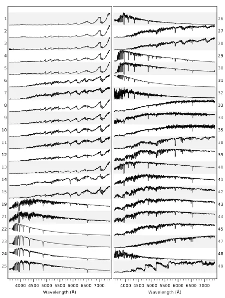
From the original set of 49 cluster spectra, we remove templates with prominent emission lines or relatively low S/N (e.g., from clusters composed of a single spectrum), leading to a final set of 42 spectra in theMILES-HC tem-plate library shown in Figure 5.29 _{We compare the}

stellar kinematics measured using the full MILES and

MILES-HClibraries in Section7.3. As one would expect, the use of MILES-HC yeilds a moderately worse fit, as determined by the fit residuals and chi-square statis-tics; however, the affect on the resulting kinematics is acceptable, particularly given the gain of roughly a fac-tor of 25 in execution time. Also, in their Section 4, Belfiore et al.,accepted, compare the emission-line mod-eling results when the stellar continuum is fit using the

MILES-HC library and various simple-stellar-population (SSP) templates. The MILES-HClibrary shows specific

27 _{Specifically, we use thescipy(Jones et al. 2001) function} cluster.hierarchy.linkage with method=’average’. This im-plements the nearest-neighbors chain hierarchical-clustering algo-rithm described byM¨ullner(2011).

28 _{Specifically, we use the}

scipy function cluster.hierarchy.fcluster with criterion=’distance’ and athresholdof 5%.

4000 4500 5000 5500 6000 6500 7000

1

2

3

4

5

6

7

8

9

10

11

12

13

14

15

19

21

22

23

24

25

Wavelength (Å)

4000 4500 5000 5500 6000 6500 7000

26

27

28

29

30

31

32

33

34

35

38

39

40

41

42

43

44

45

47

48

49

Wavelength (Å)

0.0

0.2

0.4

0.6

0.8

1.0

0.5

0.6

0.7

0.8

0.9

1.0

(>

)

7495-19xx

7495-37xx

7495-61xx

7495-91xx

7495-127xx

7495-12704

0.7 0.8 0.9

Figure 6. The fraction of valid wavelength channels (δΛ) over the full spectral range versus the fraction of spaxels (δΩ; see the definition in Section 6.1) with at least δΛ over the IFU field-of-view. Data are shown for all 17 observations from plate 7495, colored by the IFU size. The inset map showsδΛ in each spaxel of the datacube for observation 7495-12704: the hexagonal area with non-zeroδΛ is surrounded by a buffer of spaxels withδΛ = 0 resulting from the datacube construction. TheDAP only analyzes spaxels withδΛ>0.8 (vertical dashed line).

differences in the continuum shape and Balmer absorp-tion depths compared to theBruzual & Charlot(2003, BC03) library, given its lack of early-type (O) stars. However, the quality of the fits to the MaNGA spec-tra using MILES-HC are generally no worse than when using SSP templates.

6. SPATIAL BINNING

Unbiased measurements of stellar kinematics require a minimum S/N ratio, particularly for the stellar ve-locity dispersion. It is therefore generally necessary to bin spectra by averaging neighboring spaxels to meet a given S/N threshold. To bin for this purpose, we use the adaptive spatial-binning scheme implemented by the Voronoi algorithm ofCappellari & Copin(2003).30 _The

datacube construction scheme in MaNGA (Law et al. 2016, Section 9) follows the method of Shepard (1968) (cf. S´anchez et al. 2012), leading to significant covari-ance between adjacent spaxels that must be accounted for when combining spaxel data. Indeed, given that the Voronoi-binning algorithm is predicated on meeting a minimum S/N, the success of the algorithm hinges on an accurate calculation of the binned S/N. However, cal-culation of the full covariance matrix in each datacube

30 _{In DR15 specifically, we use the Python package vorbin} version3.1.3found athttps://pypi.org/project/vorbin/.

0

500 1000 1500 2000 2500 3000

0

500

1000

1500

2000

2500

3000

Flattened Map Pixel Number

Flattened Map Pixel Number

8249-12705

0.1

1

Co

rre

lat

ion

C

oe

ffi

cie

nt

,

(a)

(b)

Figure 7. The correlation matrix in channel 1132 (λ =

4700˚A) of datacube8249-12705for all spaxels with S/Ng>1. The correlation matrix is symmetric and has a correlation coefficient ofρ= 1 along the matrix diagonal, by definition. The majority of the matrix is empty withρ= 0. The inset panels provide an expanded view of two matrix subregions: Panel (a) shows ±250 pixels around the matrix center as indicated by the large gray box, and panel (b) shows±20 pixels around the matrix center as indicated by the small gray box, also shown in panel (a). The diagonal banding in panel (a) is an artifact of the ordering of adjacent pixels in the flattened vector of the datacube spatial coordinates; adjacent pixels are separated by the width of the map in one on-sky dimension. The number of bands in panel (a) roughly matches the width in pixels along the main diagonal with non-zeroρin panel (b) as expected by the spatial correlation acting along both on-sky dimensions.

is prohibitively expensive, prompting a few approxima-tions in our approach.

The following sections describe the first two modules of theDAPworkflow (Figure3) that ultimately yield the binned spectra used for the determination of the stellar kinematics. The distinction between these two mod-ules is that the first is independent of any specific bin-ning algorithm (Sections6.1 and6.2), whereas the sec-ond performs the binning itself (Sections 6.3 and 6.4). The incorporation of spatial covariance when aggregat-ing spaxels to meet a minimum S/N (Section 6.3) and when propagating the uncertainties in the binned spec-tra (Section 6.4) are treated separately for computa-tional expediency.

6.1. On-Sky Spaxel Coordinates and Datacube Mask

0

1

2

3

4

5

6

7

0.01

0.1

1

D

jk

ln

= D

/7.37

8249-12705

Figure 8. The mean (points) and standard deviation (error-bars) of the correlation coefficient,ρij, for all spaxels within the convex hull of the fiber-observation centers at channel 1132 (λ= 4700˚A) of datacube8249-12705as a function of the spaxel separation,Dij. The best-fitting Gaussian trend (red) has a scale parameter ofσ = 1.92 spaxels, leading to the equuation provided in the bottom-left corner.

center. The target center is provided in the datacube header with the keywordsOBJRAandOBJDEC.31_The

on-sky coordinates provided by the DAP are sky-right in arcseconds, with positive right-ascension offsets toward the East; note the abscissae in Figure 1 increase from right to left. The DAP then uses the photometric po-sition angle and ellipticity to calculate the semi-major-axis coordinates, R andθ. For DR15, these are simply calculated and included in the outputMAPSfile.

TheDRPalso provides detailed masks for each wave-length channel, which theDAPuses to exclude measure-ments from analysis in any given module. Large swaths of the full MaNGA spectral range can be masked by theDRPbecause of broken fibers, known foreground-star contamination, detector artifacts, or (in the majority of cases) simply because the spaxel lies outside of the hexagonal IFU field-of-view (FOV). The DAP excludes measurements affected by these issues by ignoring any measurement flagged as either DONOTUSE or FORESTAR. For each spaxel, we calculate the fraction of the MaNGA spectral range,δΛ, that is viable for analysis. For DR15, theDAP ignores any spaxel with δΛ<0.8. As a repre-sentative example, Figure6shows the viable fraction of spaxels,δΩ, withanyvalid flux measurement as a func-tion ofδΛ for the datacubes observed by plate7495.

6.2. Spectral Signal-to-Noise and Spatial Covariance

Both as a basic output product and for binning pur-poses, theDAP calculates a single measurement of S/N for each spaxel. In DR15, this fiducial S/N — hereafter referred to as S/Ng— is the average S/N per wavelength channel weighted by theg-band response function.32 _We

31 _{These are typically, but not always, the same as the pointing} center of the IFU given by the keywordsIFURAandIFUDEC.

32 _{Specifically, we use the response function produced by} Jim Gunn in 2001 provided athttps://www.sdss.org/wp-content/

calculate S/Ng for all spaxels, excluding masked chan-nels, regardless of whether or not they meet our criterion ofδΛ>0.8 (Section6.1).

For this fiducial S/Ng, we also calculate a single spa-tial covariance matrix in two steps: (1) We calculate the spatial correlation matrix for the wavelength channel at the response-weighted center of theg-band following equation 7 fromLaw et al.(2016, cf. Equation2herein). We find that the spatial correlation matrix varies weakly with wavelength over theg-band such that, to first or-der, we can simply adopt the correlation matrix from this single wavelength channel. (2) We renormalize the single-channel correlation matrix by the mean variance in the flux over the g-band to construct a covariance matrix.

Figure 7 provides the correlation matrix for wave-length channel 1132 in datacube8249-12705calculated following the first step described above, where the corre-lation coefficient is defined asρjk=Cjk/

p

CjjCkk and Cjk is the covariance between spaxels j and k. Only spaxels with S/Ng>1 are included in the Figure. Crit-ically, note that the indices j and k are not the two-dimensional indices of an individual spaxel on sky, but instead indices for the spaxels themselves. That is, spaxeljwill have on-sky coordinates (xj,yj) and appro-priate array indices in the DAPmap. This explains the diagonal banding in Figure7as an effect of spatially ad-jacent spaxels being separated by the width of the map in one dimension in the correlation matrix. Figure 7b is an expanded view of the±20 pixels about the main diagonal and has a width of approximately 10 pixels. The number of discrete diagonal bands in Figure7a and the width of the off-diagonal distribution in Figure 7b demonstrates that spaxels separated by fewer than 5 or 6 spaxels have ρ >0, consistent with the subsampling of the MaNGA 2.00_{5-diameter fiber beam into 0.}00_5×0.00₅ spaxels.

We show this explicitly in Figure 8, which combines the correlation data for all spaxels within the convex hull of the fiber centers used to construct wavelength channel 1132.33 _{We find in this case, and generally, that}

ρjkis well-fit by a Gaussian distribution in the distance between spaxels, Djk. The optimal fit to this channel is given in the Figure, where the Gaussian has a scale parameter ofσ= 1.92 spaxels (0.0096).

Finally, as a metric for the degree of covariance in this wavelength channel, we compute N2/P

jkρjk = 142.5, which provides a rough estimate of the number

uploads/2017/04/filter curves.fits with the description the SDSS Survey imaging camera at https://www.sdss.org/instruments/ camera/.

10

0

10

10

0

10

[a

rc

se

c]

[arcsec]

S/N

1

10

100

10

0

10

10

0

10

[a

rc

se

c]

[arcsec]

Ignoring Covariance

10

0

10

[arcsec]

Accounting for Covariance

0.0

2.5

5.0

7.5

10.0

12.5

15.0

17.5

10

100

Radius [arcsec]

S/

N

Figure 9. Effect of spatial covariance on the result of the Voronoi binning algorithm. The top-left panel shows the S/Ng

measurements for datacube8249-12705. We then apply the Voronoi binning algorithm to these data with a S/Ng threshold of 30. The resulting bin distribution that does not include the spatial correlation from Figure7is shown in the top-middle panel, and the bin distribution that does include the correlation is shown in the top-right panel. The colors in the top-middle and top-right panels are used to differentiate between spaxels in a given bin. The bottom panel shows the formally correct S/Ng as a function of radius for the individual spaxels (black), the bins derived assuming no covariance (red), and the bins that include the covariance (blue). The Voronoi algorithm expect the red data to have S/Ng∼30 based on the S/Ngcalculation that excludes covariances; however, the formally correct S/Ng is well below that.

of independent measurements. Note that in the limit of fully independent and fully correlated measurements, N < P

jkρjk < N2, respectively. As expected, the rough estimate of independent measurements within the datacube is comparable to the number of fibers in the relevant IFU (127); however, this is substantially smaller than the 1905 independent fiber observations used to construct the datacube. For a more in-depth discussion of datacube reconstruction and a method that minimizes datacube covariance, seeLiu et al.(2019).

6.3. Voronoi Binning with Covariance

As we have stated above, the fidelity of the Voronoi-binning approach critically depends on a proper treat-ment of the spatial covariance. For illustration purposes, we have applied the Voronoi-binning algorithm to the S/Ngmeasurements for datacube8249-12705both with and without an accounting of the spatial covariance. A map and radial profile of the S/Ng measurements are

shown in the top-left and bottom panels of Figure 9, respectively, and the correlation matrix used is shown in Figure 7. Although the threshold used in DR15 is S/Ng∼10, we use a threshold of S/Ng∼30 to accentuate the effect. Application of the algorithm without using the correlation matrix data results in the bin distribu-tion shown in the upper-middle plot of Figure 9; the distribution resulting from the formally correct S/Ng calculation is shown in the upper-right panel.

The effect of the covariance dramatically increases the number of spaxels needed to reach the target S/Ng, as evidenced by comparing the size of the bins in the upper-middle and upper-right panels. If we apply the formal calculation of the S/Ng to the bins generated without the covariance (red points in the bottom panel of Figure

Voronoi-binning algorithm, not an inconsistency in the S/N calculation. In detail, not every S/N function can partition the FOV into compact bins with equal S/N. To increase their S/N in this example, the outermost bins would have to become elongated (e.g., like a cir-cular annulus following the edge). This is prevented by the roundness criterion of the Voronoi-binning algorithm and, therefore, limits the S/Ng of these bins. However, this example is not representative of a systematic differ-ence between our target S/Ng∼10 and what is achieved by our use of the Voronoi-binning algorithm (cf. Figure

26).

To minimize the systematic errors at low S/Ng for the stellar velocity dispersions, we have chosen a S/Ng threshold of 10 per wavelength channel for DR15, which is discussed further in Section 7. This is sufficient for the first two kinematic moments, but one likely needs an increased threshold for higher order moments (h3and h4).

6.4. Spectral Stacking Calculations

For use in the subsequent modules of theDAP, the pro-cedure used to stack spaxels must yield the flux density, inverse variance, mask, and wavelength-dependent spec-tral resolution of each binned spectrum. The stacked flux density is a simple masked average of the spectra in each bin, whereas the computations for the uncertainty and spectral resolution of the binned spectra are more subtle and discussed in detail below. These procedures are fundamentally independent of the specific algorithm that determines which spaxels to include in any given bin, and our treatment of spatial covariance is slightly different.

The variance in the binned spectra is determined from the covariance matrix as follows. Similar to the calcula-tion of the covariance in the datacubes, the covariance in the binned spectra at wavelengthλis

Cλ,bin=TbinCλ,spaxelT>bin, (2)

where Cλ,spaxel is the covariance matrix for the spaxel data and Tbin is an Nbin×Nspaxel matrix where each row flags the spaxels that are collected into each bin. To avoid the expensive calculation of the full datacube covariance matrix, Law et al. (2016) — following the original proposal by Husemann et al.(2013) — recom-mended the easier propagation of the error that ignores covariance and provided a simple functional form for a factor, fcovar, that nominally recalibrates these error vectors for the effects of covariance based on the number of binned spaxels. In theDAP, we instead basefcovaron directly calculated covariance matrices sampled from 11 wavelength channels across the full spectral range of the data. As an example, Figure10shows the applied recal-ibration for the Voronoi bins in observation 8249-12705 compared to our suggested nominal calibration provided byLaw et al.(2016).

0

20

40

60

1

2

3

4

N

bin

f

co

va

r

8249-12705

Figure 10. The computed factor that properly rescales

noise vectors computed without accounting for covariance to those that do,fcovar, as a function of the number of binned

spaxels, Nbin, for the Voronoi bins constructed for

obser-vation 8249-12705 (points). These data are based on the median ratio obtained from the direct calculation of the co-variance matrix in 11 wavelength channels spanning the full spectral range of the data. For comparison, the nominal cal-ibration,fcovar= 1 + 1.62 log(Nbin), fromLaw et al. (2016)

is shown in red.

It is important to note that covariance persists in the rebinned spectra, even between large, adjacent bins.34

Therefore, it is important to account for this covariance if users wish to rebin the binned spectra;35 _{however, in}

this case, we recommend simply rebinning the original datacube.

The spectral resolution in the binned spectrum is de-termined by a nominal propagation of the per-spaxel measurements of the line-spread function (LSF), newly provided with the datacubes released in DR15 (Aguado et al. 2019). Similar to how these LSF cubes are pro-duced by theDRP, we calculate the second moment of the distribution defined by the sum of the Gaussian LSFs determined for each spaxel in the bin; i.e.,

σ_inst2 _,bin(λ) = 1 Nbin

Nbin−1

X

i

σ_inst2 _,i(λ), (3)

whereσ_inst−1_,i=Ri √

8 ln 2/λ for each spaxeli, with reso-lutionRi, in the bin. A limitation of this calculation is that the assumption of a Gaussian LSF with a dispersion of σ2

inst,bin for the binned spectrum becomes less accu-rate as the range inσinst,i increases. For MaNGA data, the variation in the LSF between spaxels in a datacube is generally only a few percent, meaning that this should

34 _{It is effectively impossible to rebin the MaNGAdatacubein} a way that removes the covariance. One has to restart with the fiber data in theRSSfiles.