The data reduction pipeline for the SDSS IV MaNGA IFU Galaxy Survey

THE DATA REDUCTION PIPELINE FOR THE SDSS-IV MaNGA IFU GALAXY SURVEY

David R. Law1, Brian Cherinka2, Renbin Yan3, Brett H. Andrews4, Matthew A. Bershady5, Dmitry Bizyaev6, Guillermo A. Blanc7,8,9, Michael R. Blanton10, Adam S. Bolton11, Joel R. Brownstein11, Kevin Bundy12,

Yanmei Chen13,14, Niv Drory15, Richard D’Souza16, Hai Fu17, Amy Jones16, Guinevere Kauffmann16, Nicholas MacDonald18, Karen L. Masters19, Jeffrey A. Newman4, John K. Parejko18, José R. Sánchez-Gallego3,

Sebastian F. Sánchez20, David J. Schlegel21, Daniel Thomas19, David A. Wake5,22, Anne-Marie Weijmans23, Kyle B. Westfall19, and Kai Zhang3

1

Space Telescope Science Institute, 3700 San Martin Drive, Baltimore, MD 21218, USA;dlaw@stsci.edu 2

Center for Astrophysical Sciences, Department of Physics and Astronomy, Johns Hopkins University, Baltimore, MD 21218, USA 3

Department of Physics and Astronomy, University of Kentucky, 505 Rose Street, Lexington, KY 40506-0055, USA 4

Department of Physics and Astronomy and PITT PACC, University of Pittsburgh, 3941 O’Hara Street, Pittsburgh, PA 15260, USA 5

Department of Astronomy, University of Wisconsin-Madison, 475 N. Charter Street, Madison, WI 53706, USA 6

Apache Point Observatory, P.O. Box 59, Sunspot, NM 88349, USA 7

Departamento de Astronomía, Universidad de Chile, Camino del Observatorio 1515, Las Condes, Santiago, Chile 8

Centro de Astrofísica y Tecnologías Afines(CATA), Camino del Observatorio 1515, Las Condes, Santiago, Chile 9

Visiting Astronomer, Observatories of the Carnegie Institution for Science, 813 Santa Barbara Street, Pasadena, CA, 91101, USA 10_{Center for Cosmology and Particle Physics, Department of Physics, New York University, 4 Washington Place, New York, NY 10003, USA}

11

Department of Physics and Astronomy, University of Utah, 115 S 1400 E, Salt Lake City, UT 84112, USA 12

Kavli Institute for the Physics and Mathematics of the universe, Todai Institutes for Advanced Study, the University of Tokyo, Kashiwa, 277-8583(Kavli IPMU, WPI), Japan

13

School of Astronomy and Space Science, Nanjing University, Nanjing 210093, China 14

Key Laboratory of Modern Astronomy and Astrophysics(Nanjing University), Ministry of Education, Nanjing 210093, China 15

McDonald Observatory, Department of Astronomy, University of Texas at Austin, 1 University Station, Austin, TX 78712-0259, USA 16

Max Planck Institute for Astrophysics, Karl-Schwarzschild-Str. 1, D-85748 Garching, Germany 17

Department of Physics & Astronomy, University of Iowa, Iowa City, IA 52242, USA 18

Department of Astronomy, Box 351580, University of Washington, Seattle, WA 98195, USA 19

Institute of Cosmology and Gravitation, University of Portsmouth, Portsmouth, UK

20_{Instituto de Astronomia, Universidad Nacional Autonoma de Mexico, A.P. 70-264, 04510 Mexico D.F., Mexico} 21

Physics Division, Lawrence Berkeley National Laboratory, Berkeley, CA 94720-8160, USA 22

Department of Physical Sciences, The Open University, Milton Keynes, UK 23

School of Physics and Astronomy, University of St. Andrews, North Haugh, St. Andrews KY16 9SS, UK

Received 2016 April 5; revised 2016 May 27; accepted 2016 June 9; published 2016 September 12

ABSTRACT

Mapping Nearby Galaxies at Apache Point Observatory (MaNGA)is an optical fiber-bundle integral-field unit (IFU)spectroscopic survey that is one of three core programs in the fourth-generation Sloan Digital Sky Survey (SDSS-IV). With a spectral coverage of 3622–10354Å and an average footprint of ∼500 arcsec2 per IFU the scientific data products derived from MaNGA will permit exploration of the internal structure of a statistically large sample of 10,000 low-redshift galaxies in unprecedented detail. Comprising 174 individually pluggable science and calibration IFUs with a near-constant data stream, MaNGA is expected to obtain ∼100 million raw-frame spectra and∼10 million reduced galaxy spectra over the six-year lifetime of the survey. In this contribution, we describe the MaNGA Data Reduction Pipeline algorithms and centralized metadata framework that produce sky-subtracted spectrophotometrically calibrated spectra and rectified three-dimensional data cubes that combine individual dithered observations. For the 1390 galaxy data cubes released in Summer 2016 as part of SDSS-IV Data Release 13, we demonstrate that the MaNGA data have nearly Poisson-limited sky subtraction shortward of

∼8500Åand reach a typical 10σlimiting continuum surface brightnessμ=23.5 AB arcsec−2in afi ve-arcsecond-diameter aperture in theg-band. The wavelength calibration of the MaNGA data is accurate to 5 km s−1rms, with a median spatial resolution of 2.54 arcsec FWHM (1.8 kpc at the median redshift of 0.037)and a median spectral resolution of σ=72 km s−1.

Key words:methods: data analysis –surveys –techniques: imaging spectroscopy

1. INTRODUCTION

Over the last 20 yr, multiplexed spectroscopic surveys have been valuable tools for bringing the power of statistics to bear on the study of galaxy formation. Using large samples of tens to hundreds of thousands of galaxies with optical spectroscopy from the Sloan Digital Sky Survey(York et al.2000; Abazajian et al. 2003), for instance, studies have outlined fundamental relations between stellar mass, metallicity, element abundance ratios, and star formation history(e.g., Kauffmann et al.2003; Tremonti et al. 2004; Thomas et al. 2010). However, this

statistical power has historically come at the cost of treating galaxies as point sources, with only a small and biased region subtended by a given opticalfiber contributing to the recorded spectrum.

As technology has advanced, techniques have been devel-oped forimaging spectroscopythat allow simultaneous spatial and spectral coverage, with correspondingly greater informa-tion density for each individual galaxy. Building on early work by(e.g.)Colina et al.(1999)and de Zeeuw et al.(2002), such integral-field spectroscopy has provided a wealth of informa-tion. In the nearby universe, for instance, observations from the

DiskMass survey (Bershady et al. 2010) have indicated that late-type galaxies tend to have sub-maximal disks (Bershady et al. 2011), while Atlas-3D observations (Cappellari et al. 2011a) showed that early-type galaxies frequently have rapidly rotating components (especially in low-density envir-onments; Cappellari et al.2011b). In the more distant universe, integral-field spectroscopic observations have been crucial in establishing the prevalence of high gas-phase velocity disper-sions(e.g., Förster Schreiber et al.2009; Law et al.2009,2012; Wisnioski et al.2015), giant kiloparsec-sized clumps of young stars(e.g., Förster Schreiber et al.2011), and powerful nuclear outflows (Förster Schreiber et al. 2014) that may indicate fundamental differences in gas accretion mechanisms in the young universe (e.g., Dekel et al.2009).

More recently, surveys such as the Calar Alto Legacy Integral Field Area Survey (CALIFA, Sánchez et al. 2012; García-Benito et al. 2015), Sydney-AAO Multi-object IFS (SAMI, Croom et al. 2012; Allen et al. 2015) and Mapping Nearby Galaxies at Apache Point Observatory (MaNGA, Bundy et al. 2015) have begun to combine the information density of integral-field spectroscopy with the statistical power of large multiplexed samples. As a part of the fourth generation of the Sloan Digital Sky Survey (SDSS-IV), the MaNGA project bundles single fibers from the Baryon Oscillation Spectroscopic Survey(BOSS)spectrograph(Smee et al.2013)

into integral-field units(IFUs); over the six-year lifetime of the survey (2014–2020) MaNGA will obtain spatially resolved optical+NIR spectroscopy of 10,000 galaxies at redshifts

z∼0.02–0.1. In addition to providing insight into the resolved structure of stellar populations, galactic winds, and dynamical evolution in the local universe (e.g., Belfiore et al. 2015; Li et al.2015; Wilkinson et al.2015), the MaNGA data set will be an invaluable legacy product with which to help understand galaxies in the distant universe. As next-generation facilities come online in the final years of the MaNGA survey, IFU spectrographs such as TMT/IRIS(Moore et al. 2014; Wright et al.2014),James Webb Space Telescope(JWST)/NIRSPEC (Closs et al. 2008; Birkmann et al. 2014), andJWST/ MIRI-MRS (Wells et al. 2015) will trace the crucial rest-optical bandpass in galaxies out to redshiftz∼10 and beyond.

Imaging spectroscopic surveys such as MaNGA face substantial calibration challenges in order to meet the science requirements of the survey(R. Yan et al.2016b). In addition to requiring accurate absolute spectrophotometry from eachfiber, MaNGA must correct for gravitationally induced flexure variability in the Cassegrain-mounted BOSS spectrographs, determine accurate micron-precision astrometry for each IFU bundle, and combine spectra from the individual fibers with accurate astrometric information in order to construct three-dimensional (3D) data cubes that rectify the wavelength-dependent differential atmospheric refraction (DAR) and (despite large interstitial gaps in thefiber bundles)consistently deliver high-quality imaging products. These combined requirements have driven a substantial software pipeline development effort throughout the early years of SDSS-IV.

Historically, IFU data have been processed with a mixture of software tools ranging from custom built pipelines (e.g., Zanichelli et al. 2005) to general-purpose tools capable of performing all or part of the basic data reduction tasks for multiple IFUs. For fiber-fed IFUs (with or without coupled lenslet arrays)that deliver a pseudo-slit of discrete apertures, the raw data are similar in format to traditional multi-object

spectroscopy and have hence been able to build upon an existing code base. In contrast, slicer-based IFUs produce data in a format more akin to long-slit spectroscopy, while pure-lenslet IFUs are different altogether with individual spectra staggered across the detector.

Following Sandin et al. (2010), we provide here a brief overview of some of the common tools for the reduction of data from optical and near-IR IFUs (see also Bershady 2009), including both fiber-fed IFUs with data formats similar to MaNGA and lenslet- and slicer-based IFUs by way of comparison. As shown in Table 1, the IRAF environment remains a common framework for the reduction of data from many facilities, especially Gemini, WIYN, and William Herschel Telescope(WHT). Similarly, the various IFUs at the Very Large Telescope(VLT)can all be reduced with software from a commonISO C-based pipeline library, although some other packages(e.g., GIRBLDRS, Blecha et al.2000)are also capable of reducing data from some VLT IFUs. Substantial effort has been invested in theP3D(Sandin et al.2010)andR3D (Sánchez2006)packages as well, which together are capable of reducing data from a wide variety of fiber-fed instruments (including PPAK/LARR, VIRUS-P, SPIRAL, GMOS, VIMOS, INTEGRAL, and SparsePak) for which similar extraction and calibration algorithms are generally possible. For survey-style operations, the SAMI survey has adopted a two-stage approach, combining a general-purpose spectro-scopic pipeline 2DFDR(Hopkins et al.2013)with a custom 3D stage to assemble IFU data cubes from individualfiber spectra (Sharp et al.2015).

Similarly, the MaNGA Data Reduction Pipeline (MANGADRP; hereafter the DRP) is also divided into two components. Like the KUNGIFU package (Bolton & Burles 2007), the two-dimensional (2D) stage of the DRP is based largely on the SDSS BOSS spectroscopic reduction pipelineIDLSPEC2D(D. Schlegel et al. 2016, in preparation), and processes the raw CCD data to produce sky-subtracted,

flux-calibrated spectra for eachfiber. The 3D stage of the DRP is custom built for MaNGA, but adapts core algorithms from the CALIFA (Sánchez et al. 2012) and VENGA (Blanc et al. 2013) pipelines in order to produce astrometrically registered composite data cubes. In the present contribution, we describe version v1_5_4 of the MaNGA DRP corresponding to thefirst public release of science data products in SDSS Data Release 13(DR13).24

We start by providing a brief overview of the MaNGA hardware and operational strategy in Section 2, and give an overview of the DRP and related systems in Section3. We then discuss the individual elements of the DRP in detail, starting with the basic spectral extraction technique(including detector pre-processing,fiber tracing,flat-field, and wavelength calibra-tion) in Section 4. In Section 5 we discuss our method of subtracting the sky background (including the bright atmo-spheric OH features)from the science spectra, and demonstrate that we achieve nearly Poisson-limited performance shortward of 8500Å. In Section 6 we discuss the method for spectro-photometric calibration of the MaNGA spectra, and in Section7

our approach to resampling and combining all of the individual spectra onto a common wavelength solution. We describe the astrometric calibration in Section 8, combining a basic approach that takes into account fiber bundle metrology,

24

DAR, and other factors (Section 8.1), and an “extended” astrometry module that registers the MaNGA spectra against SDSS-I broadband imaging (Section 8.2). Using this astro-metric information we combine together individual fiber spectra into composite 3D data cubes in Section 9. Finally, we assess the quality of the MaNGA DR13 data products in Section 10, focusing on the effective angular and spectral resolution, wavelength calibration accuracy, and typical depth of the MaNGA spectra compared to other extant surveys. We summarize our conclusions in Section 11. Additionally, we provide an AppendixBin which we outline the structure of the MaNGA DR13 data products and quality-assessment bitmasks.

2. MANGA HARDWARE AND OPERATIONS

2.1. Hardware

The MaNGA hardware design is described in detail by Drory et al. (2015); here we provide a brief summary of the major elements that most closely pertain to the DRP. MaNGA uses

the BOSS optical fiber spectrographs (Smee et al. 2013)

installed on the Sloan Digital Sky Survey 2.5 m telescope (Gunn et al.2006)at Apache Point Observatory(APO)in New Mexico. These two spectrographs interface with a removable cartridge and plugplate system; each of the six MaNGA cartridges contains a full complement of 1423fibers that can be plugged into holes in pre-drilled plug plates ∼0.7 m (3°) in diameter and which feed pseudo-slits that align with the spectrograph entrance slits when a given cartridge is mounted on the telescope.

These 1423 fibers are bundled into IFUs ferrules with varying sizes; each cartridge has 12 seven-fiber IFUs that are used for spectrophotometic calibration and 17 science IFUs of sizes varying from 19 to 127fibers(see Table 2). As detailed by D. Wake et al. (in preparation), this assortment of sizes is chosen to best correspond to the angular diameter distribution of the MaNGA target galaxy sample. The orientation of each IFU on the sky isfixed by use of a locator pin and pinhole a short distance west of the IFU. Additionally, each IFU ferrule

Table 1

IFU Data Reduction Software

Telescope Spectrograph IFU Pipeline Reference

Fiber-fed IFUs

AAT AAOMEGA SAMI 2DFDR Sharp et al.(2015)

Calar Alto 3.5 m PMAS PPAK P3D Sandin et al.(2010)

R3D Sánchez(2006)a

IRAF Martinsson et al.(2013)b

HET VIRUS VIRUS CURE Snigula et al.(2014)

McDonald 2.7 m VIRUS-P VIRUS-P VACCINE Adams et al.(2011)

VENGA Blanc et al.(2013)

SDSS 2.5 m BOSS MaNGA MANGADRP This paper

WHT WYFFOS INTEGRAL IRAF

WIYN WIYN Bench Spec. DensePak IRAF Andersen et al.(2006)

SparsePak IRAF

Fiber+Lenslet-based IFUs

AAT AAOMEGA SPIRAL 2DFDR Hopkins et al.(2013)

Calar Alto 3.5 m PMAS LARR As PPAK above

Gemini GMOS GMOS IRAF

Magellan IMACS IMACS KUNGIFU Bolton & Burles(2007)

VLT GIRAFFE ARGUS GIRBLDRS Blecha et al.(2000)

ESO CPLc

VIMOS VIMOS VIPGI Zanichelli et al.(2005)

ESO CPLc

Lenslet-based IFUs

Keck OSIRIS OSIRIS OSIRISDRP Krabbe et al.(2004)

UH 2.2 m SNIFS SNIFS SNURP

WHT OASIS OASIS XOASIS

SAURON SAURON XSAURON Bacon et al.(2001)

Slicer-based IFUs

ANU WiFeS WiFeS IRAF Dopita et al.(2010)

Gemini GNIRS GNIRS IRAF

NIFS NIFS IRAF

VLT KMOS KMOS ESO CPLc,SPARK Davies et al.(2013)

MUSE MUSE ESO CPLc Weilbacher et al.(2012)

SINFONI SINFONI ESO CPLc Modigliani et al.(2007)

Notes. a

See Sánchez et al.(2012)for details of the implementation for the CALIFA survey. b

Reference corresponds to the DiskMass survey. c

has a complement of associated sky fibers (see Table 2)

amounting to a total of 92 individually pluggable skyfibers. Each fiber is 150μm in diameter, consisting of a 120μm glass core surrounded by a doped cladding and protective buffer. The 120μm core diameter subtends 1.98 arcsec on the sky at the typical plate scale of ∼217.7 mm degree−1. These

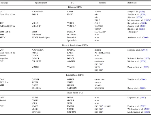
fibers are terminated into 44 V-groove blocks with 21–39fibers each that are mounted on the two pseudo-slits. As illustrated in Figure1, the skyfibers associated with each IFU are located at the ends of each block to minimize crosstalk from adjacent science fibers. In total, spectrograph 1(2)is fed by 709(714) individual fibers.

Within each spectrograph a dichroic beamsplitter reflects light blueward of 6000Åinto a blue-sensitive camera with a 520 l/mm grism and transmits red light into a camera with a 400 l/mm grism (both grisms consist of a VPH transmission grating between two prisms). There are therefore four“frames” worth of data taken for each MaNGA exposure, one each from the cameras b1/b2(blue cameras on spectrograph 1/2)and r1/ r2 (red cameras on spectrograph 1/2). The blue cameras use blue-sensitive 4K×4K e2V CCDs while the red cameras use 4K×4K fully depleted LBNL CCDs, all with 15 micron pixels(Smee et al.2013). The combined wavelength coverage of the blue and red cameras is∼3600–10300Å, with a 400Å overlap in the dichroic region (see Table 3 for details). The typical spectral resolution ranges from 1560 to 2650, and is a function of the wavelength, telescope focus, and the location of an individual fiber on each detector (see, e.g., Figure 37 of Smee et al. 2013); we discuss this further in Sections 4.2.5

and 10.2.

While each of the IFUs is assigned a specific plugging location on a given plate, the sky fibers are plugged non-deterministically(although all are kept within 14 arcmin of the galaxy that they are associated with). Each cartridge is mapped after plugging by scanning a laser along the pseudo-slitheads and recording the corresponding illumination pattern on the plate. In addition to providing a complete mapping of fiber number to on-sky location, this also serves to identify any broken or mispluggedfibers. This information is recorded in a central svn-based metadata repository calledMANGACORE(see Section 3.3).

2.2. Operations

Each time a plate is observed, the cartridge on which it is installed is wheeled from a storage bay to the telescope and mounted at the Cassegrain focus. Observers acquire a given

field using a set of 16 coherent imagingfibers that feed a guide

camera; these provide the necessary information to adjust focus, tracking, plate scale, andfield rotation using bright guide stars throughout a given set of observations. In addition to simple tracking, constant corrections are required to compen-sate for variations in temperature and altitude-dependent atmospheric refraction.

At the start of each set of observations, the spectrographs are

first focused using a pair of hartmann exposures; the best focus is chosen to optimize the line spread function(LSF)across the entire detector region(see Sections 4.2.2and 4.2.5).

Twenty-five-second quartz calibration lampflat-fields and four-second Neon–Mercury–Cadmium arc-lamp exposures are then obtained by closing the eight flat-field petals covering the end of the telescope. These provide information on thefi

ber-to-fiber relative throughput and wavelength calibration, respec-tively; since both are mildly flexure dependent they are repeated every hour of observing at the relevant hour angle and declination.

After the calibration exposures are complete, science exposures are obtained in sets of three 15 minute dithered exposures. As detailed by Law et al. (2015), this integration time is a compromise between the minimum time necessary to reach background limited performance in the blue while simultaneously minimizing astrometric drift due to DAR between the individual exposures. Since MaNGA is an imaging spectroscopic survey, image quality is important and the 56%

fill factor of circular fiber apertures within the hexagonal MaNGA IFU footprint(Law et al.2015)naturally suffers from substantial gaps in coverage. To that end, we obtain data in “sets” of three exposures dithered to the vertices of an equilateral triangle with 1.44 arcsec to a side. As detailed by Law et al.(2015), this provides optimal coverage of the target

field and permits complete reconstruction of the focal plane image. Since atmospheric refraction (which is wavelength dependent, time-dependent through the varying altitude and parallactic angle, and field dependent through uncorrected quadrupole scale changes over our 3° field) degrades the uniformity of the effective dither pattern, each set of three exposures is obtained in a contiguous hour of observing.25 These sets of three exposures are repeated until each plate reaches a summed signal-to-noise ratio (S/N) squared of 20 pixel−1fiber−1ing-band atg=22 AB and 36 pixel−1fiber−1 ini-band ati=21 AB(typically 2–3 hr of total integration; see R. Yan et al.2016b).

All MaNGA galaxy survey observations are obtained in dark or gray-time for which the moon illumination is less than 35% or below the horizon(see R. Yan et al.2016bfor details). Since MaNGA shares cartridges with the infrared SDSS-IV/ APO-GEE spectrograph, however (Wilson et al. 2010), both instruments are able to collect data simultaneously. MaNGA and APOGEE therefore typically co-observe, meaning that data are also obtained with the MaNGA instrument during bright-time with up to 100% moon illumination. These bright-bright-time data are not dithered, have substantially higher sky back-grounds, and are generally used for ancillary science observa-tions of bright stars with the aim of amassing a library of stellar reference spectra over the lifetime of SDSS-IV. These bright-time data are processed with the same MaNGA software

Table 2

MaNGA IFU Complement Per Cartridge

IFU size Purpose Number Nsky

a

Diameterb

(fibers) of IFUs (arcsec)

7 Calibration 12 1 7.5

19 Science 2 2 12.5

37 Science 4 2 17.5

61 Science 4 4 22.5

91 Science 2 6 27.5

127 Science 5 8 32.5

Notes. a

Number of associated skyfibers per IFU ferrule. b

Total outer-diameter IFU footprint.

25

pipeline as the dark-time galaxy data, albeit with some modifications and unique challenges that we will address in a future contribution.

3. OVERVIEW: MANGA DRP

In this section we give a broad overview of the MaNGA DRP and related systems in order to provide a framework for the detailed discussion of individual elements presented in Sections4–9.

3.1. Data Reduction Pipeline

The MaNGA DRP is tasked with producing fully fl ux-calibrated data for each galaxy that has been spatially rectified and combined across all individual dithered exposures in a multi-extension FITS format that may be used for scientific analysis. ThisMANGADRPsoftware is written primarily in IDL, with some C bindings for speed optimization and a variety of python-based automation scripts. Dependencies include the SDSSIDLUTILSand NASA Goddard IDL astronomy users libraries; namespace collisions with these and other common libraries have been minimized by ensuring that non-legacy DRP routines are prefixed by either“ml_”or“mdrp_.”The DRP runs automatically on all data using the collaboration supercluster at the University of Utah,26is publicly accessible in a subversionSVN repository at

https://svn.sdss.org/public/repo/manga/mangadrp/tags/v1_5_ 4with a BSD three-clause license, and has been designed to run on individual users’ home systems with relatively little over-head.27Version control of theMANGADRPcode and dependencies is done via SVN repositories and traditional trunk/branch/tag methods; the version of MANGADRPdescribed in the present contribution corresponds to tag v1_5_4 for public release DR13. We note that v1_5_4 is nearly identical to v1_5_1 (which has been used for SDSS-IV internal release MPL-4) save for minor

Figure 1.Schematic diagram of a 127fiber IFU on MaNGA galaxy 7495–12704. The left-hand panel shows the SDSS three-color RGB image of the galaxy overlaid with a hexagonal bounding box showing the footprint of the MaNGA IFU. The right-hand panel shows a zoomed-in grayscaleg-band image of the galaxy overlaid with circles indicating the locations of each of the 127 optical sciencefibers(colored circles)and schematic locations of the 8 skyfibers(black circles). Thesefibers are grouped into four physical blocks on the spectrograph entrance slit(schematic diagram at bottom), with the skyfibers located at the ends of each block. Note that the orientation of thisfigure isflipped in relation to Figure9 of Drory et al.(2015)as the view presented here is on-sky(north up, east left).

Table 3

BOSS Spectrograph Detectors

Blue Cameras Red Cameras

Type e2V LBNL fully depleted

Grism(l/mm) 520 400

Wavel. Range(Å)a 3600–6300 5900–10300

Resolutiona 1560–2270 1850–2650

Detector Size 4352×4224 4352×4224

Active Pixelsb [128:4223, 56:4167] [119:4232, 48:4175]

Pixel Size(μm) 15 15

Read noise(e-/pixel)a ∼2.0 ∼2.5

Gain(e-/ADU)a ∼1.0 ∼1.5–2.0

Notes. a

Values are approximate; see Smee et al.(2013)for details. b

Zero-indexed locations of active pixels between overscan regions.

26

Presently 27 nodes with 16 CPUs per node. 27

improvements in cosmic-ray rejection routines and data-quality-assessment statistics.

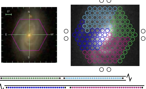
The DRP consists of two primary parts: the 2D stage that produces flux-calibrated fiber spectra from individual expo-sures, and the 3D stage that combines individual exposures with astrometric information to produce stacked data cubes. The overall organization of the DRP is illustrated in Figure 2. Each day when new data are automatically transferred from APO to the SDSS-IV central computing facility at the University of Utah a cronjob triggers automated scripts that run the 2D DRP on all new exposures from the previous modified Julian date(MJD). These are processed on a per-plate basis, and consist of a mix of science and calibration exposures (flat-fields and arcs).

The 2D stage of the MaNGA DRP is largely derived from the BOSSIDLSPEC2Dpipeline(see, e.g., Dawson et al.2013, Schlegel et al., in preparation)28 that has been modified to address the different hardware design and science requirements of the MaNGA survey(we summarize the numerous differences in AppendixA). Each frame undergoes basic pre-processing to remove overscan regions and variable-quadrant bias before the one-dimensional

(1D)fiber spectra are extracted from the CCD detector image. The DRPfirst processes all of the calibration exposures to determine the spatial trace of thefiber spectra on the detector and extractfiber

flat-field and wavelength calibration vectors, and applies these to the corresponding science frames. The science exposures are in turn extracted, flatfielded, and wavelength calibrated using the corresponding calibrationfiles. Using the skyfibers present in each exposure we create a super-sampled model of the background sky spectrum, and subtract this off from the spectra of the individual sciencefibers. Finally, the 12 mini-bundles targeting standard stars in each exposure are used to determine theflux calibration vector for the exposure compared to stellar templates. Thefinal product of the 2D stage is a single FITS file per exposure (mgCFrame) containing row-stacked spectra (RSS; i.e., a 2D array in which each row corresponds to an individual 1D spectrum)of each of the 1423 fibers interpolated to a common wavelength grid and combined across the four individual detectors.

Once a sufficient number of exposures has been obtained on a given plate, it is marked as complete at APO and a second automated script triggers the 3Dstage DRP to combine each of the mgCFramefiles resulting from the 2D DRP. For each IFU (including calibration mini-bundles)on the plate, the 3D pipeline identifies the relevant spectra in the mgCFrame files and assembles them into a master row-stacked format consisting of

Figure 2.Schematic overview of the MaNGA data reduction pipeline. The DRP is broken into two stages: mdrp_reduce2d and mdrp_reduce3d. The 2D pipeline data products areflux-calibrated individual exposures corresponding to an entire plate; the 3D pipeline products are summary data cubes and row-stacked spectra for a given galaxy combining information from many exposures.

28_The

all spectra for that target. The astrometric solution as a function of wavelength for each of these spectra is computed on a per-exposure basis using the knownfiber bundle metrology and dither offset for each exposure, along with a variety of other factors including field and chromatic differential refraction (see Law et al. 2015). This astrometric solution is further refined using SDSS broadband imaging of each galaxy to adjust the position and rotation of the IFU fiber coordinates. Using this astrometric information the DRP combines the fiber spectra from individual exposures into a rectified data cube and associated inverse variance and mask cubes. In post-processing, the DRP addition-ally computes mock broadbandgrizimages derived from the IFU data, estimates of the reconstructed point-spread function(PSF)at

griz, and a variety of quality-control metrics and reference information.

The final DRP data products in turn feed into the MaNGA Data Analysis Pipeline (DAP), which performs spectral modeling, kinematic fitting, and other analyses to produce science data products such as Hα velocity maps, kinemetry, spectral emission line ratio maps, etc., from the data cubes. DAP data products will be made public in a future release and described in a forthcoming contribution by K. Westfall et al.(in preparation).

3.2. Quick-reduction Pipeline(DOS)

Rather than running the full DRP in real-time at the observatory, we instead use a pared-down version of the code that has been optimized for speed that we refer to as DOS.29The DOS pipeline shares much of its code with the DRP, performing reduction of the calibration and science exposures up through sky subtraction. The primary difference is in the spectral extraction; while the DRP performs an optimized profilefitting technique to extract the spectra of eachfiber(see Section4.2.2), DOS instead uses a simple boxcar extraction that sacrifices some accuracy and robustness for substantial gains in speed.

The primary purpose of DOS is to provide real-time feedback to APO observers on the quality and depth of each exposure. Each exposure is characterized by an effective depth given by the mean S/N squared at afixedfiber2mag30of 22(g -band) and 21 (i-band). The S/N of each fiber is calculated empirically by DOS from the sky-subtracted continuumfluxes and inverse variances, while nominalfiber2mags for eachfiber in a galaxy IFU are calculated by applying aperture photometry to SDSS broadband imaging data at the known locations of each of the IFU fibers (see Section 8.1) and correcting for Galactic foreground extinction following Schlegel et al.(1998). As illustrated in Figure 3, the S/N as a function offiber2mag for all fibers in a given exposure forms a logarithmic relation that can befitted and extrapolated to the effective achieved S/N at fixed nominal magnitudes g = 22 and i = 21. This calculation is done independently for all four cameras using a

g-band effective wavelength range λλ4000–5000Åand an i -band effective wavelength range λλ6910–8500Å. As described above in Section 2.2, we integrate on each plate until the cumulative S/N2 in all complete sets of exposures

reaches 20 pixel−1fiber−1ing-band and 36 pixel−1fiber−1in

i-band at the nominal magnitudes defined above.

3.3. Metadata

MaNGA is a complex survey that requires tracking of multiple levels of metadata (e.g., fiber bundle metrology, cartridge layout, fiber plugging locations, etc.), any of which may change on the timescale of a few days(in the case offiber plugging locations) to a few years (if cartridges and/or fiber bundles are rebuilt). At any point, it must be possible to rerun any given version of the pipeline with the corresponding metadata appropriate for the date of observations. This metadata must also be used throughout the different phases of the survey from planning and target selection, to plate drilling, to APO operations, to eventual reduction and post-processing.

To this end, MaNGA maintains a central metadata repository MANGACORE, which is automatically synchronized between APO and the Utah data reduction hub using daily crontabs. Version control offiles withinMANGACOREis maintained by a combination of MJD datestamps and periodic SVN tags corresponding to major data releases(v1_2_3 for DR13).

3.4. Quality Control

Given the volume of data that must be processed by the MaNGA pipeline (∼10 million reduced galaxy spectra and

∼100 million raw-frame spectra over the six-year lifetime of SDSS-IV31), automated quality control is essential. To that end, multiple monitoring routines are in place. The 2D and 3D stage DRP has bitmasks (MANGA_DRP2PIXMASK and MAN-GA_DRP3PIXMASK, respectively) associated with the pri-mary flux extensions that can be used to indicate individual pixels(or spaxels32 in the case of the 3D data cubes)that are identified as problematic. In the 2D case(spectra of all 1423 individual fibers within a single exposure), this pixel mask indicates such things as cosmic-ray events, bad flat-fields, missing fibers, extraction problems, etc. In the 3D stage (a

Figure 3.S/N as a function of extinction-correctedfiber magnitude for blue

(left panel)and red cameras(right panel), for spectrographs 1 and 2(diamond vs. square symbols, respectively). The red line indicates the logarithmic relation derived fromfitting points in the magnitude range indicated by the vertical dotted lines. Thefilled red circle indicates the derivedfit at the nominal magnitudes g=22 and i=21, with the S/N2 _{values given for each} spectrograph. This example corresponds to MaNGA plate 7443, MJD 56741, exposure 177378.

29

Daughter-of-Spectro. This pipeline is a sibling to the Son-of-Spectro quick-reduction pipeline used by the BOSS and eBOSS surveys, both of which are descended from the original SDSS-I Spectro pipeline.

30

Fiber2mag is a magnitude measuring theflux contained within a 2 arcsec diameter aperture; see http://www.sdss.org/dr13/algorithms/magnitudes/ #mag_fiber.

31

Assuming an average of three clear hours per night between the bright and dark-time programs, five exposures per hour (including calibrations), and

∼3000 spectra per exposure among four individual CCDs. 32

composite cube for a single galaxy that combines many individual exposures into a regularized grid), this pixel mask indicates things like low/no fiber coverage, foreground star contamination, and other issues that mean a given spaxel should not be used for science.

Additionally, there are overall quality bits MANGA_DRP2Q-UAL and MANGA_DRP3QMANGA_DRP2Q-UAL that pertain to an entire exposure or data cube, respectively, and indicate potential issues during processing. In the 2D case, this can include effects like heavy cloud cover, missing IFUs, or abnormally high scattered light. In the 3D case, this can include warnings for bad astrometry, bad flux calibration, or (rarely) a critical problem suggesting that a galaxy should not be used for science. As of DR13, 22 of the 1390 galaxy data cubes areflagged as critically problematic for a variety of reasons ranging from the severe and unrecoverable (e.g., poor focus due to hardware failure, ∼5 objects) to the potentially recoverable in a future data release (e.g., failed astrometric registration due to a bright star at the edge of the IFU bundle) to the mundane (errant unflagged cosmic-ray confusing the flux calibration QA routine).

All of these pixel-level and exposure-level data qualityflags are used by the pipeline in deciding how and whether to continue to process data (e.g., flux calibration will not be attempted on an exposure flagged as completely cloudy). We provide a reference table of the key MaNGA quality-control bitmasks in AppendixB.4.

4. SPECTRAL EXTRACTION

MaNGA exposures are differentiated from BOSS/eBOSS exposures taken with the same spectrographs using FITS header keywords, and a planfile33is created for each plate on a given MJD detailing each of the exposures obtained for which the quality was deemed by DOS at APO to be excellent. The MaNGA DRP parses this planfile and performs pre-processing, spectral extraction, flatfielding, wavelength calibration, sky subtraction, andflux calibration on a per-exposure basis.

4.1. Pre-processing

Raw data from each of the four CCDs(b1, r1, b2, r2)are in the format of 16 bit images with 4352 columns and 4224 rows (Table3), with a 4096 ×4112 pixel active area(for the blue CCDs; 4114 ×4128 pixel active area for the red CCDs) and overscan regions along each edge of the detector. As described by Dawson et al. (2013), the CCDs are read out with four amplifiers, one for each quadrant, resulting in variable bias levels. Each exposure is preprocessed to remove the overscan regions of the detector, subtract off quadrant-dependent biases, convert from bias corrected ADUs to electrons using quadrant-dependent gain factors derived from the overscan regions,34 and divide by aflat-field containing the relative pixel-to-pixel response measured from a uniformly illuminated calibration image (see Figure 4).

A corresponding inverse variance image is created using the measured read noise and photon counts in each pixel; this inverse variance array is capped so that no pixel has a reported

S/N greater than 100.35 Finally, potential cosmic rays(which affect∼ 10 times as many pixels in the red cameras as in the blue) are identified and flagged using the same algorithm adopted previously by the SDSS imaging and spectroscopic surveys. As discussed by R.H. Lupton(seehttp://www.astro. princeton.edu/~rhl/photo-lite.pdf), this algorithm is a fi rst-pass approach that successfully detects most cosmic rays by looking for features sharper than the known detector PSF, but sometimes incompletely flags pixels around the edge of cosmic-ray tracks. A second-pass approach that addresses these residual features is applied later in the pipeline, as described in Section7. The inverse variance image is combined with this cosmic-ray mask and a reference bad pixel mask so that affected pixels are assigned an inverse variance of zero (and hence have zero weight in the reductions).

4.2. Calibration Frames

All flat-field and arc calibration frames from a planfile are reduced prior to processing any science frames. These provide estimates of the fiber-to-fiber flat-field and the wavelength solution, and are also critical for determining the locations of individual fiber spectra on the detectors. Since there are four cameras, each reducedflat-field (arc)exposure corresponds to four mgFlat(mgArc)multi-extension FITSfiles as described in the data model in AppendixB.

4.2.1. Spatial Fiber Tracing

As illustrated in Figure4, MaNGAfibers are arranged into blocks of 21–39 fibers with 22 blocks on each spectrograph, with individual spectra running vertically along each CCD. The

fiber spacing within blocks is 177μm for science IFUs (∼4 pixels), and 204μm for spectrophotometric calibration IFUs, with ∼624μm between each block. Fibers are initially identified in a uniformly illuminated flat-field image using a cross-correlation technique to match the 1D profile along the middle row of the detector against a referencefile describing the nominal location of eachfiber in relative pixel units. The cross-correlation technique matching against all fibers on a given slit allows for shifts due to flexure-based optical distortions while ensuring robustness against missing or broken individual fibers and/or entire IFUs. Fibers that are missing within the central row areflagged as dead inMANGACORE.

With the initialx-positions of eachfiber in the central row thus determined, the centroids of eachfiber in the other rows are then determined using aflux-weighted mean with a radius of 2 pixels. This algorithm sequentially steps up and down the detector from the central row, using the previous row’s position as the initial input to the flux-weighted mean. Fibers with problematic centroids(e.g., due to cosmic rays)are masked out, and replaced with estimates based on neighboring traces. These

flux-weighted centroids are further refined using a per-fiber cross-correlation technique matching a Gaussian model fiber profile (see Section 4.2.2) against the measured profile in a given row. Thisfine adjustment is required in order to remove sinusoidal variations in theflux-weighted centroids at the∼0.1 pixel level caused by discrete jumps in the pixels included in the previousflux-weighted centroiding.

Once the positions of all fibers across all rows of the detector have been computed, the discrete pixel locations are

33

A planfile is a plaintext asciifile that is both machine and human readable

(seehttp://www.sdss.org/dr13/software/par/) and contains a list of the science and calibration exposures to be processed through a given stage of the pipeline.

34

Typical read noise and detector gains are given in Table3; these are slightly different for each quadrant of each detector, and can evolve over the lifetime of the survey. See Smee et al.(2013)for details.

35

stored as a traceset36 of seventh-order Legendre polynomial coefficients. An iterative rejection method accounts for scatter and uncertainty in the centroid measurement of individual rows and ensures realistically smooth variation of a given

fiber trace as a function of wavelength along the detector. The best-fit traceset coefficients are stored as an extension in the per-camera mgFlat files(Table5).

4.2.2. Spectral Extraction

Similarly to the BOSS survey (Dawson et al. 2013), we extract individual fiber spectra from the 2D detector images using a row-by-row optimal extraction algorithm that uses a least-squares profilefit to obtain an unbiased estimate of the total counts(Horne1986). The counts in each row are modeled

by a linear combination ofN_fiberGaussian

37

profiles plus a low-order polynomial (or cubic basis-spline; see Section 4.2.3)

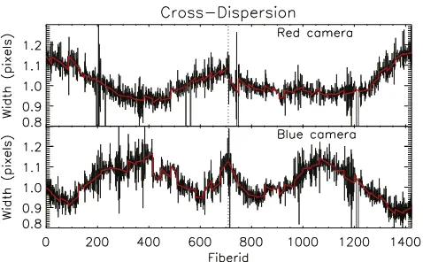
background term. As we illustrate in Figure5(right panel), the resulting model is an extremely goodfit to the observed profile. MaNGA uses the extract_row.c code (dating back to the original SDSS spectroscopic survey), which creates a pixelwise model of the Gaussian profile integrated over fractional pixel positions (i.e., the profile is assumed to be Gaussian prior to pixel convolution), describes deviations to the line centers and widths as linear basis modes(representing thefirst and second spatial derivatives, respectively), and solves for the banded matrix inversion by Cholesky decomposition. An initialfit to theflat-field calibration images allows both the amplitude and the width of the Gaussian profiles in each row to vary freely, with the centroid set to the positions determined via fiber tracing in Section4.2.1. These individual width measurements are noisy, however, and for each block offibers we thereforefit the derived widths with a linear relation as a function offiberid along the slit in order to reject errant values and determine a

fixed set of fiber widths that vary smoothly (within a given

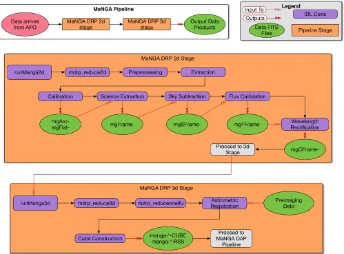
Figure 4.Illustration of the MaNGA raw data format before(A)and after(B)pre-processing to remove the overscan and quadrant-dependent bias. This image shows a color-inverted typical 15 minute science exposure for the b1 camera(exposure 177378 for plate 7443 on MJD 56741). There are 709 individualfiber spectra on this detector, grouped into 22 blocks. Bright spectra represent central regions of the target galaxies and/or spectrophotometric calibration stars; bright horizontal features are night-sky emission lines. Panel C zooms in on 10 blocks in the wavelength regime of the bright[OI5577]skyline.

36

A traceset is a set of coefficient vectors defining functions over a common independent-variable domain specified by “xmin” and “xmax” values. The functions in the set are defined in terms of a linear combination of basis functions (such as Legendre or Chebyshev polynomials) up to a specified maximum order, weighted by the values in the coefficient vectors, and evaluated using a suitable affine rescaling of the dependent-variable domain

(such as[xmin, xmax][−1, 1]for Legendre polynomials). For evaluation purposes, the domain is assumed by default to be a zero-based integer baseline from xmin to xmax such as would correspond to a digital detector pixel grid.

37

block) with both fiberid and wavelength. As illustrated in Figure 6, low-frequency variation of the widths with fiberid reflects the telescope focus(which we choose to ensure that the widths are as constant as possible across the entire slit), while discontinuities at the block boundaries are due to slight differences in the slithead mounting. These fixed widths are then used in a secondfit to the detector images in which only the polynomial background and the amplitude of the Gaussian terms are allowed to vary.

Thefinal value adopted for the totalflux in each row is the integral of the theoretical Gaussian profile fits to the observed pixel values, while the inverse variance is taken to be the diagonal of the covariance matrix from the Cholesky decom-position. This approach allows us to be robust against cosmic rays or other detector artifacts that cover some fraction of the spectrum, since unmasked pixels in the cross-dispersion profile can still be used to model the Gaussian profile (Figure 5). Additionally, this technique naturally allows us to model and subtract crosstalk arising from the wings of a given profile overlapping any adjacentfibers, and to estimate the variance on the extracted spectra at each wavelength. This step transforms our 4096×4112 CCD images(4114×4128 for the red cameras)to RSS with dimensionality 4112×N_fiber(4128×Nfiberfor the red cameras).

4.2.3. Scattered Light

The DRP automatically assesses the level of scattered light in the MaNGA data by taking advantage of the hardware design in which gaps of ∼16 pixels were left between each v-groove block(compared to∼4 pixels peak-to-peak between each fiber trace within a block)so that the interstitial regions contain negligible light from the Gaussian fiber profile cores (Drory et al. 2015). By masking out everything within five pixels of the fiber traces we can identify those pixels on the edge of the detector and in empty regions between individual blocks whose counts are dominated by diffuse light on the detector. This light is a combination of (1) genuine scattered light that enters the detector via multiple reflections from unbaffled surfaces and(2)highly extended non-Gaussian wings to the individual fiber profiles that can extend to hundreds of pixels and contain∼1%–2% of the total light of a givenfiber.

For MaNGA dark-time science exposures (which typically peak at about 30 counts pixel−1fiber−1for the sky continuum) both components are small and can be satisfactorily modeled by a low-order polynomial term in each extracted row. For some bright-time exposures used in the stellar library program, however, the moon illumination can approach 100% and produce larger scattered light counts ∼ a quarter of the sky background seen by individualfibers. Additionally, for ourfl

at-field calibration exposures the summed contribution of the non-Gaussian wings to the fiber profiles can reach ∼300 counts pixel−1in the interstial regions between blocks (compared to

∼20,000 counts pixel−1in thefiber profile cores). In both cases the simple polynomial background term can prove unsatisfac-tory, and we insteadfit the counts in the interstitial regions row-by-row with a fourth-order basis-spline model that allows for a greater degree of spatial variability in the background than is warranted for the dark-time science exposures. This bspline model is evaluated at the locations of each intermediate pixel and smoothed along the detector columns by use of a 10 pixel

Figure 5.Left panel: cross-dispersionflat-field profile cut for the R1 camera. Gray points lie withinfive pixels of the measuredfiber traces, black points are more than five pixels from the nearestfiber trace. The solid red line indicates the bsplinefit to the inter-block values. Right panel: Cross-dispersion profile zoomed in around CCD column 900. The solid black line shows the individual pixel values, the solid red line overplots the Gaussian profilefiberfit plus the bspline background term convolved with the pixel boundaries. The trough around pixel 900–910 represents a gap between V-groove blocks. Both panels show row 2000 from plate 8069 observed on MJD 57278.

moving boxcar to mitigate the impact of individual bad pixels. The resulting bspline scattered light model is subtracted from the raw counts before performing spectral extraction.

4.2.4. Fiber Flat-field

Each flat-field calibration frame is extracted into individual

fiber spectra using the above techniques and matched to the nearest (in time) arc-lamp calibration frame, which has been processed as described in Section 4.2.5. Using the wavelength solutions derived from the arc frames, we combine the individual

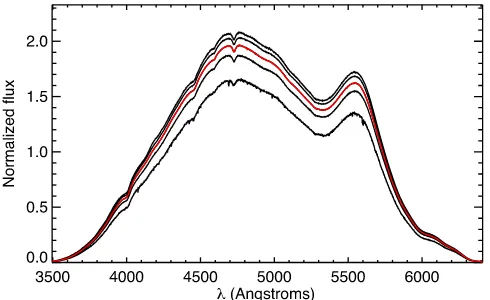
flat-field spectra (first normalized to a median of unity) into a single composite spectrum with substantially greater spectral sampling than any individual fiber.38 We fit this composite spectrum with a cubic basis-spline function to obtain the superflat vector describing the global flat-field response (i.e., the quartz lamp spectrum convolved with the detector response and system throughput). This global superflat is shown in Figure 7, and illustrates the falloff in system throughput toward the wavelength extremes of the detector(see also Figure4 of Yan et al.2016a). We evaluate the superflat spline function on the native wavelength grid of each individualfiber and divide it out from the individualfiber spectra in order to obtain the relativefi ber-to-fiber flat-field spectra. So normalized, these fiber-to-fiber

flat-field spectra have values near unity, vary only slowly(if at all)with wavelength, and easily show any overall throughput differences between the individual fibers. Each such spectrum is in turn fitted with a bspline in order to minimize the contribution of photon noise to the resulting fiber flats and interpolate across bad pixels. In the end, we are left with two

flat-fields to store in the mgFlat files (see Table 5); a single

superflatspectrum describing the global average response as a function of wavelength, and a fiberflatof size 4112 × N_fiber

(4128 × N_fiber for the red cameras) describing the relative throughput of each individualfiber as a function of wavelength. The individual MaNGAfibers typically have high throughput (see discussion by Drory et al.2015) within 5%–10% of each other. The relative distribution of throughputs is monitored daily to trigger cleaning of the IFU surfaces when the DRP detects noticeable degradation in uniformity or overall throughput. Individualfibers with throughput less than 50% that of the best

fiber on a slit areflagged by the pipeline and ignored in the data analysis. This may occur when afiber and/or IFU falls out of the plate(a rare occurrence), or when afiber breaks. Such breakages in the IFU bundles occur at the rate of about 1fiber per month across the entire MaNGA complement of 8539fibers.

4.2.5. Wavelength and Spectral Resolution Calibration

The Neon–Mercury–Cadmium arc-lamp spectra are extracted in the same manner as theflat-fields, except that they use thefiber traces determined from the corresponding flat-field (with allowance for a continuous 2D polynomial shift in the traces as a function of detector position to account forflexure differences) and allow only the Gaussian profile amplitudes to vary. These spectra are normalized by the fiber flat-field39 and an initial wavelength solution is computed as follows.

A representative spectrum is constructed from the median of thefive closest spectra closest to the centralfiber on the CCD. This spectrum is cross-correlated with a model spectrum generated using a reference table of known strong emission features in the Neon–Mercury–Cadmium arc lamps,40 and iterated to determine the best-fit coefficients to map pixel locations to wavelengths. These best-fit coefficients are used to contruct initial guesses for the wavelength solution of each

fiber, which are then iterated on afiber-to-fiber basis to obtain thefinal wavelength solutions. Several rejection algorithms are run to ensure reliable arc-line centroids across allfibers. Afinal sixth-order Legendre polynomial fit converts the wavelength solutions into a series of polynomial traceset coefficients. The higher order coefficients are forced to vary smoothly as a function offiberid since they predominantly arise from optical distortions along the slit(whereas lower order terms represent differences arising from thefiber alignment). These coefficients are stored as an extension in the output mgArc file (see Table4), and are used to reconstruct the wavelength solutions at allfibers and positions on the CCD.

The arc-lamp spectral resolution (hereafter the line spread function, or LSF)is computed byfitting the extracted spectra around the strong arc-lamp emission lines in eachfiber with a Gaussian profile integrated over each pixel (note that we

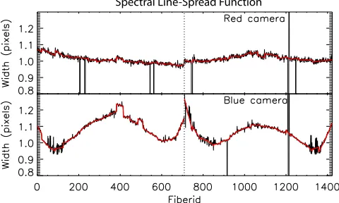
integrate thefitted profile shape across each pixel rather than simply evaluating the profile at the pixel midpoints; see the discussion in Section 10.2) and allowing both the width and amplitude of the profile to vary. As illustrated in Figure8, these widths are intrinsically noisy and the DRP therefore fits them with a linear relation as a function offiberid along the slit in order to reject errant values and determine afixed set of line widths that vary smoothly(within a given block)withfiberid. These arc-line widths are thenfit with a Legendre polynomial traceset that is stored in the mgArcfiles and evaluated at each pixel to compute the LSF at wavelengths between the bright arc lines.

Both wavelength and LSF solutions derived from the arc frames are later adjusted for each individual science frame to account for instrumental flexure during and between (see discussion in Section4.3).

Figure 7.Example of a typical superflat spectrum for the b1 camera normalized to a median of unity. The solid red line shows the superflatfit to the median fiber, solid black lines indicate the 1σand 2σdeviations about this median.

38

Since eachfiber has a slightly different wavelength solution we effectively supersample the intrinsic input spectrum.

39

In practice this is iterative; theflat-fields prior to separation of the superflat and fiberflat are used to normalize the arc-lamp spectra, the wavelength solution from which in turn allows construction of the superflat.

40

All calibrations are additionally complicated in the red cameras since the middle row of pixels on these detectors is oversized by a factor of 1/3, causing a discontinuity in both the wavelength solution and the LSF for eachfiber as a function of pixel number. All of the algorithms described above therefore allow for such a discontinuity across the CCD quadrant boundary. The primary impact of this discontinuity on thefinal data products is to produce a spike of low spectral resolution around 8100Å, the exact wavelength of which can vary from

fiber tofiber based on the curvature of the wavelength solution along the detector.

4.3. Science Frames

Each science frame is associated with the arc and flat pair taken closest to it in time (generally within one hour since calibration frames are taken at the start of each plate and periodically thereafter), and extracted row-by-row following the method outlined in Section 4.2.2. During this extraction only the profile amplitudes and background polynomial term are allowed to vary freely; the trace centroids are tied to the

flat-field traces with a global 2D polynomial shift to account for instrumentflexure, and the cross-dispersion widths arefixed to the values derived from theflat-field. The extracted spectra are normalized by the superflat and fiberflat vectors derived from theflat-field.

The wavelength solutions derived from the arcs are adjusted for each science frame to match the known wavelengths of bright night-sky emission lines in the science spectra byfitting a low-order polynomial shift as a function of detector position to allow for instrumentalflexure(these shifts are typically less than a quarter pixel). The final wavelength solution for each exposure is corrected to the vacuum heliocentric restframe using header keywords recording atmospheric conditions and the time and date of a given pointing. As we explore in Section 10.3, we achieve a ∼10 km s−1or better rms wave-length calibration accuracy with zero systematic offset to within 2 km s−1.

Similarly, in order to account for flexure and varying spectrograph focus with time the spectral LSF measurements derived from the arc-lamp exposures are also adjusted for each science frame to match the LSF of bright skylines that are known to be unblended in high-resolution spectra (e.g., Osterbrock et al. 1996). Starting from the original arc-line

LSF model, we derive a quadrature correction term for the profile widthsQ2=s -s

sky2 arc2.Qis taken to be constant as a function of wavelength for each camera, and is based on the strong auroral OI5577 line in the blue(since the HgIlines are too weak and broadened to obtain a reliablefit)and an average of many isolated bright lines in the red.41 The measured quadrature correction term isfitted with a cubic basis-spline to ensure that the correction applied varies smoothly withfiberid. Across the ∼1100 individual exposures in DR13 the average correction Q2 =0.08 ± 0.04 pixel2 in the blue cameras and

= 

Q2 0.05 0.02_pixel2_{in the red cameras(likely due to the}

flatter and more stable focus in the red cameras).

The final RSS, inverse variances, pixel masks, wavelength solutions, and broadened LSF are all stored as extensions in the output mgFrame FITSfile(Table6).

5. SKY SUBTRACTION

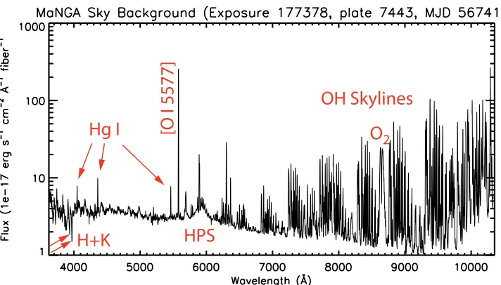
Unlike previous SDSS spectroscopic surveys targeting bright central regions of galaxies, MaNGA will explore out to…2.5 effective radii (Re) where galaxy flux is decreasing rapidly relative to the sky background. As illustrated in Figure9, this night-sky background is especially bright at near-IR wave-lengths longward of ∼8000Å, where bright emission lines from OH radicals (e.g., Rousselot et al. 2000) dominate the backgroundflux. These OH features vary in strength with both time and angular position depending on the coherence scale of the atmosphere, posing challenges for measuring faint stellar atmospheric features such as the Wing–Ford (Wing & Ford

1969)band of iron hydride absorption lines around 9900Å. In many cases such faint features will be detectable only in stacked bins of spectra, driving the need to reach the Poisson-limited noise regime so that stacked spectra are not Poisson-limited by systematic sky subtraction residuals.

We therefore design our approach to sky subtraction with the aim of reaching Poisson-limited performance at all wavelengths from λλ4000–10000Å (beyond which the increasing read noise of the BOSS cameras prohibits such performance). Our sky subtraction algorithm is closely based on the routines developed for the BOSS survey, and relies on using the dedicated 92 skyfibers(46 per spectrograph)on each plate to construct a highly sampled model background sky that can be subtracted from each of the sciencefibers. These skyfibers are plugged into regions identified during the plate design process as blank sky“objects”within a 14 arcmin patrol radius of their associated IFUfiber bundle(see Figure1).

5.1. Sky Subtraction Procedure

Sky subtraction is performed independently for each of the four cameras using theflat-fielded, wavelength-calibratedfiber spectra contained in the mgFrame files, and is a multi-step iterative process. Broadly speaking, we build a super-sampled sky model from all of the sky fibers, scale it to the sky background level of a given block, and evaluate it on the native solution of eachfiber within that block. In detail:

1. The metadata associated with the exposure are used to identify theNskyindividual skyfibers in each frame based on their FIBERTYPE.

Figure 8.As Figure6, but showing the spectral line spread function(1σLSF) for the Gaussian arc-line profile as a function offiberid for an emission line near the middle row of all four detectors (CdI 5085.822Å for the blue cameras, NeI8591.2583Åfor the red cameras).

41

2. Pixel values for these Nskysky fibers are resorted as a function of wavelength into a single one-dimensional array of lengthNsky×Nspec(whereNspecis the length of a single spectrum). Since each fiber has a unique wavelength solution, this super-sky vector has much higher effective sampling of the night-sky background spectrum than any individual fiber and provides an accurate LSF for OH airglow features. An example of this procedure is shown in Figure10.

3. Similarly, we also construct a super-sampled weight vector by comining individual skyfiberinverse variance spectra that have first been smoothed by a boxcar of width 100 pixels (∼100–200Å)in the continuum and 2 pixels (∼2–3Å) within 3Å of bright atmospheric emission features.

4. The super-sky spectrum is then weighted by the smoothed inverse variance spectrum (convolved with the bad-pixel mask)andfitted with a cubic basis-spline as a function of wavelength, with the number of breakpoints set to~Nspecso that high-frequency variations (due, e.g., to shot noise or bad pixels)are not picked up by the resulting model(see, e.g., green line in Figure10).42The breakpoint spacing is set automatically to maintain approximately constant S/N between breakpoints. The B-spline fit itself is iterative, with upper and lower rejection threshholds set to mask bad or deviant pixels. We note that the smoothing of the inverse variance in determining the weight function is critical as otherwise the weights(which are themselves estimated from the data)would modulate with the Poisson scatter and bias the fit toward slightly lower values, resulting in systematic undersubtraction of the sky background, especially near the wavelength extrema where the overall system throughput is low.

5. This B-spline function is evaluated on the native wavelength solution of each of the sky fibers. Dividing the original sky fiber spectra by this functional model,

and collapsing over wavelengths using a simple mean, we arrive at a series of scale factors describing the relative sky background seen by thefiber compared to all other

fibers on the detector. For each harness (i.e., each IFU plus associated sky fibers) we compute the median of these scale factors to obtain a single averaged scale factor for each harness. These scale factors help account for nearly gray variations in the true sky continuum across our large field produced by a combination of intrinsic background variations and patchy cloud cover. The variability in sky background between harnesses is about 1.5% rms, with some larger deviations >5% observed during the bright-time stellar library program when pointing near a full moon can produce strong background gradients.

6. Repeat steps 2–4 after first scaling each individual sky

fiber spectrum by the value appropriate for its harness in order to obtain a super-sky spectrum in which per-harness scaling effects have been removed.

7. Evaluate the new B-spline function on the native pixelized wavelength solution of each fiber (sky plus science), and multiply it by the scaling factor for the harness to obtain the first-pass model sky spectrum for each fiber. Subtract this from the spectra to obtain the

first-pass sky-subtracted spectra.

8. Identify deviant sky fibers in which the median sky-subtracted residual S/N2>2(this is extremely rare, and generally corresponds to a case where a skyfiber location was chosen poorly, or a fiber was misplugged and not corrected before observing). Eliminate these sky fibers from consideration, and repeat steps 2–7 to obtain the second-pass model sky spectrum for eachfiber. We refer to this as the 1D sky model.

9. Repeat steps 2–4, this time allowing the bspline fit to accommodate a smoothly varying third-order polynomial of values at each breakpoint as a function offiberid(i.e., rather than requiring the model to be constant for allfibers, it is allowed to vary slowly as a function of slit position). This polynomial term is introduced in order to model

Figure 9.Typicalflux-calibrated MaNGA night-sky background spectrum seen by a single opticalfiber(2 arcsec core diameter). Bright features longward of 7000Å represent blended OH and O2skyline emission(see, e.g., Osterbrock et al.1996). The bright feature at 5577Åis atmospheric[OI], the broad feature around 6000Åis high-pressure sodium(HPS)from streetlamps; HgIfrom Mercury vapor lamps contributes most of the discrete features at short wavelengths(see, e.g., Massey & Foltz2000). Absorption features around 4000Åare zodiacal Fraunhofer H and K lines.

42

variations in the LSF along each slit; empirically, increasing polynomial orders up to three results in an improvement of the skyline residuals, while no further gains are observed at greater than third order. Evaluate the new B-spline function on the native pixelized wavelength solution of eachfiber(sky plus science)to obtain the 2D sky model. Notably, this 2D model does not use the explicit scaling used by the 1D model. This is partially because a similar degree of freedom is introduced by the 2D polynomial, and partially because OH features can vary in strength independently from the underlying continuum background(see, e.g., Davies2007).

10. Thefinal sky model is a piecewise hybrid of the 1D and 2D models; in continuum regions it is taken to be the 1D model, and in the skyline regions(i.e., within 3Åof any wavelength for which the sky background is>5σabove a bsplinefit to the interline continuum)it is taken to be the 2D model. We opt for this hybrid model as it optimizes our various performance metrics: In the continuum far from night-sky lines, our performance is limited by the poisson-based rms of the model sky spectrum subtracted from each sciencefiber. Therefore, we use the 1D model that is based on all 46 skyfibers on a given spectrograph. In contrast, for near bright skylines our performance is instead limited by our ability to accurately model the shape of the skyline wings, which can vary along the slit (see, e.g., Figure8). Therefore, in skyline regions we use the 2D model, which improves the model LSFfidelity at the expense of some S/N. There is no measurable discontinuity between the sky-subtracted spectra at the piecewise 1D/2D model boundaries.

Thefinal sky model is subtracted from the mgFrame spectra; these sky-subtracted spectra are stored in mgSFrame files (Table 7), which contain the spectra, inverse variances (with appropriate error propagation), pixel masks, applied sky models, etc. in a row-stacked format identical to the input mgFramefiles.

5.2. Sky Subtraction Performance: All-sky Plates

We estimate the accuracy of our calibration and sky subtraction up to this point by using specially designed“ all-sky”plates in which every science IFU is placed on a region of sky determined to be empty of visible sources according to the SDSS imaging data(calibration mini-bundles are still placed on standard stars so that these all-sky plates can be properlyflux calibrated). The resulting sky-subtracted sky spectra can then be used to estimate the accuracy of our noise model, extraction algorithms, and sky-subtraction technique.

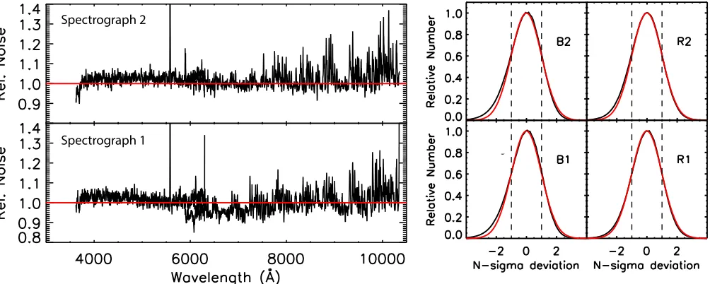
Working with the row-stacked mgSFrame spectra(i.e., prior toflux calibration and wavelength rectification) we construct “Poisson ratio”images for each camera by multiplying the sky-subtracted residual counts by the square root of the inverse variance(which accounts for both shot noise and detector read noise). If the sky subtraction is perfect, and the noise model properly estimated, these poisson ratio images should be devoid of structure with a Gaussian distribution of values with mean of 0 and σ =1.0. In Figure 11 (right-hand panels)we show the actual distribution of values for the sky-subtracted science fibers for exposure 183643 (cart 4, plate 8069, MJD 56901) for each of the four cameras (solid black lines) compared to the ideal theoretical expectations(solid red line; note that this isnotafit to the data). We find that the overall distribution of values is broadly consistent with theoretical models in all four cameras (c.f. Figure23 of Newman et al.2013, which shows similar plots for the DEEP2 survey), albeit with some evidence for slight oversubtraction on average and a non-Gaussian wing in the blue cameras (pixels in this asymmetric wing do not correspond to particular wavelengths orfiberid).

We examine this behavior as a function of wavelength in Figure 11 (left-hand panel) by plotting the 1σ width of the Gaussian that bestfits the distribution of unflagged pixel values at a given wavelength across all science fibers.43 As before, perfectly noise-limited sky subtraction with a perfect noise model would correspond to aflat distribution ofσaround 1.0 at all wavelengths; we note that the blue cameras and the continuum regions of the r2 camera are close to this level of performance with up to a 3% offset from nominal(suggesting that the read noise in some quadrants may be marginally underestimated). In the r1 camera the read noise may be overestimated by∼10% in some quadrants(asσ<1 for r1 in the wavelength rangeλλ5700–7600Å), but is otherwise well-behaved in the continuum region. In the skyline regions of the red cameras, performance is within 10% of Poisson expecta-tions out to∼8500Å. Longward of∼8500Å (where skylines are brighter, and the spectra have greater curvature on the detectors) sky subtraction performance in skyline regions is

∼10%–20% above theoretical expectations. This is likely due to systematic residuals in the subtraction caused by block-to-block variations in the spectral LSF that are difficult to model completely. Indeed, such an analysis during commissioning revealed the OH skyline residuals were significantly worse in R1 than in the R2 camera. This led to the discovery of an optical coma in R1 that wasfixed during Summer 2014 prior to the formal start of SDSS-IV, but which nonetheless affected the commissioning plates 7443 and 7495.

Figure 10.Example MaNGA super-sky spectrum created by the wavelength-sorted combination of all-sky fiber spectra(black line)in the OH-emission dominated wavelength region λλ7900–7960Å. Overlaid in green is the b-spline modelfit to the super-sky spectrum; red points represent the b-spline model after evaluation on the native pixellized wavelength solution of a singlefiber.

43