Long run commodity prices, economic growth and interest rates: 17th century to the present day

(1)

Long-Run Commodity Prices, Economic Growth and

Interest Rates: 17th Century to the Present Day

David I. Harvey (University of Nottingham), Neil M. Kellard

(University of Essex), Jakob B. Madsen (Monash University) and

Mark E. Wohar (University of Nebraska at Omaha)

July 2016

Abstract

A significant proportion of the trade basket of many developing countries is prised of primary commodities. This implies relative price movements in com-modities may have important consequences for economic growth and poverty reduction. Taking a long-run perspective, we examine the historical relation be-tween a new aggregate index of commodity prices, economic activity and interest rates. Initial empirical tests show that commodity prices present a downward trend with breaks over the entire industrial age, providing clear support for the Prebisch-Singer hypothesis. It would also appear that this trend has declined at a faster rate since the 1870s. Conversely, several GDP series such as World, Chile, China, UK and US, trend upwards with breaks. Such trending behaviour in both commodity prices and economic activity suggests a latent common factor like technological innovation.

(2)

More-over, commodity price movements have an asymmetric country effect on economic

activity; periods of falling commodity prices will support GDP growth for

com-modity importers like the US but depress growth for comcom-modity exporters such

as Chile.

Keywords: Primary commodities; Prebisch-Singer hypothesis; Economic growth; Interest rates; Structural breaks; VAR.

JEL Classification: O13; C22.

1 Introduction

A significant proportion of national income for many developing countries is often

generated by a small number of primary commodities (see Harveyet al., 2010), leading

to a possible resource curse.1 _{The nature and causes of any long-run trends and}

short-run movements in primary commodity prices therefore have significant implications for

growth and poverty reduction policies in developing countries.

Analysis of long-run commodity prices is dominated by the Prebisch-Singer (PS)

hypothesis which implies a secular, negative trend in commodity prices relative to

manufactures.2 Possible theoretical rationales include low income elasticities of de-mand for commodities, asymmetric market structures that result from comparatively

homogeneous commodity producers generating highly competitive commodity markets

whilst facing oligopolistic manufacturing markets, and technological and

productiv-ity differentials between core (industrial) and periphery (non-industrial) countries. If

a country’s export commodities present long-run downward trends in their relative

prices, the policy advice is typically to diversify the export mix to include significant

(3)

(2014a), understanding the trend and other time series characteristics should enable

improved forecasting of commodity price movements.

Empirical evidence examining the PS hypothesis provides an ambiguous picture.

The vast majority of recent studies employ the Grilli and Yang (1988) dataset of 24

annual non-fuel primary commodity prices which commences in 1900.3 _{However, the}

relatively large variance of commodity prices (see Deaton, 1999) and the possibility

of trend structural breaks inhibits statistical determination of any trend magnitude

and direction with this sample size. A possible approach to address this issue is to

provide greater degrees of freedom via a backwards extension of the sample. Recently,

Harveyet al. (2010) and Arezkiet al. (2014b) employ a unique disaggregated dataset,

comprised of 25 separate commodity time series and spanning the 17th to the 21st

centuries.

Compared to long-run trends, shorter term fluctuations in commodity prices are

relatively under-researched in the literature. This is surprising given that commodity

prices are known to be extremely volatile, leading to uncertainty over future revenue

and cost streams. This uncertainty may inhibit planning and deter investment by

all the relevant agents in the commodity supply chain (i.e., household farmers,

coop-eratives, larger commercial farmers and governments). The shortfalls in investment

subsequently act as a drag on future growth and poverty reduction prospects (see

Blattmanet al., 2007 and Poelhekke and van der Ploeg, 2009). Additionally, although

severe price movements may be temporary in character, permanent and detrimental

effects on physical and cognitive development, particularly during early childhood, can

arise in commodity dependent communities (see, inter alia, Pongou et al., 2006 and

Miller and Urdinola, 2010).

Some studies have attempted to identify the macroeconomic variables that influence

(4)

structural approach of Gilbert (1989) and Chu and Morrison (1986) demonstrated that

two demand side variables, the US dollar real exchange rate and industrial production

of industrialised countries, adequately explained movements in commodity prices over

the early 1980s. After 1984, when industrial countries started to recover from

reces-sion, this demand-side framework failed to explain the continuing weakness in prices.

In response, Borensztein and Reinhart (1994) extended the traditional framework to

include supply side factors, the relative price of oil and a new definition of demand,

encompassing output changes from Eastern Europe and the Soviet Union. The model

greatly improved empirical explanation of commodity price movements over the 1980s

and early 1990s. More recent work, such as Arango et al. (2012), stresses that economic

activity and interest rates are the primary determinants of commodity prices.

Papers attempting to explain movements in commodity prices typically use post

World War 2 data. For example, the aforementioned Arango et al. (2012), employs

annual data from 1960 to 2006. Our paper takes a different tack by examining

rela-tionships between commodity prices, economic activity and interest rates over the very

long-run. To do so, we first create an aggregate index for real commodity prices. This

is achieved by collecting a large historical dataset on the export values of 23 individual

commodities; not a straightforward task. These new data are then used as weights

when combined with updated individual commodity series from Harvey et al. (2010)

to construct the aggregate annual series beginning in 1650 and running continuously

until 2014. Additionally, data for interest rates are obtained from the Bank of England,

whilst historical GDP data (i.e., for the World and various individual countries) are

obtained from the Maddison Project.

As a precursor to the multivariate approach, our second contribution is to examine

the time series properties, and in particular the trend, of the long-run series. Given

the well known problems of identifying the order of integration of commodity price

(5)

subsequent tests of commodity time series characteristics (see Harveyet al., 2010), we

apply trend tests and multiple trend break tests which are robust to whether or not the

series under consideration contains a unit root. The results show that the trend path

of our new aggregate commodity series can be split into four regimes (i.e., 1650 to the

early 1820s, the early 1820s to the early 1870s, the early 1870s to the mid-1940s, and

the mid-1940s to 2014). Through all but the second regime, a long-run downward trend

can be clearly detected, giving new historical support to the PS hypothesis. Moreover,

although prices present a secular decline over the 17th and 18th centuries, this was at

a slower rate as compared with the 20th century. The economic forces behind the PS

hypothesis would appear to have intensified during the 1900s.

In terms of economic activity, it is shown that UK GDP presents an upward trend

break in the 1820s and World GDP in the 1870s and 1950s. Interestingly, these dates are

closely associated with those found for commodity prices. Additionally, the increasing

rate of trend growth in GDP as the sample increases, mirrors the decreasing rate

of trend growth for commodity prices, suggesting a common latent factor such as

technological innovation.

Our third contribution is to model the relationships between our long-run series.

The data are first demeaned and detrended according to the breaks found in the prior

time series analysis. These detrended series are shown to be stationary and therefore,

unlike other recent literature which does not allow for breaks, a cointegration approach

is not appropriate. Using a stationary VAR (Vector Autoregression), there is evidence

that (detrended) commodity prices Granger cause (detrended) GDP and interest rates,

whilst interest rates Granger cause commodity prices. Such results have implications

for the resource curse and the effect of monetary policy.

The remainder of the paper is organised as follows. Section 2 outlines the theory

and empirical methodology, whilst section 3 describes the new data. The empirical

(6)

2 Theory and Empirical Methodology

2.1 Demand and supply in the commodity market

The theory of either long-run trend or cyclical movements about the trend are not well

developed or evidenced (see Deaton and Laroque, 2003). As noted in the introduction,

rationales for the trend include low income elasticities of demand for commodities,

technological and productivity differentials or asymmetric market structures between

the oligopolistic, manufacturing core and the competitive, commodity producing south.

Additionally, new discoveries of commodities and technological innovation4in commod-ity production will increase supply and reduce costs respectively, also placing downward

pressure on the trend in commodity prices. Movements around any trend, and

includ-ing macroeconomic variables mentioned by the literature such as economic activity

(see Borenszstein and Reinhart, 1994) and interest rates (see Frankel, 2006), might

be described by the following partial equilibrium model. Using a standard log-linear

demand function (see Deaton and Laroque, 2003), it can be written that:

dt=αyt−βpt+γ+εdt (1)

where dt is demand, yt represents the logarithm of world income. and pt is the world

price for an internationally traded commodity. Moreover, a complimentary supply

function (see Arango et al., 2012) can be stated:

pt=δst−1+ηrt−1+θpt+εst (2)

(7)

where st is current supply as a function of last period’s supply and rt represents the

interest rate. In equilibrium, supply is equal to demand, and it can be shown that:

pt= (β+δ)−1[αyt+γ−δst−1+ηrt−1+εdt −ε s

t] (3)

where (3) suggests that commodity prices around any trend are related to income,

interest rates and supply. Of course, before examining any multivariate association,

the time series properties of each individual series requires investigation. Given we will

employ very long-run data, breaks in the individual data generating processes (DGP)

are likely. Therefore, the following sections will outline our testing procedure for trends

and any breaks in trends and levels.

2.2 Testing for a linear trend

We initially consider the following DGP for zt, the logarithm of a variable of interest:

zt=α+βt+ut, t = 1, ..., T (4)

ut=ρut−1+εt, t= 2, ..., T (5)

with u1 =ε1, whereεt is assumed to follow a stationary process. To permit the errors

ut to be either I(0) or I(1), we assume −1 < ρ≤ 1, with the cases |ρ| <1 and ρ = 1

corresponding to I(0) and I(1) errors, respectively. Given that we are interested in

examining issues like the PS hypothesis, the null hypothesis to be tested isH0 :β = 0,

and we wish to conduct tests on this hypothesis without assuming knowledge of whether

the errors ut are stationary or contain a unit root.

In the context of such a DGP, Perron and Yabu (2009a) propose tests ofH0 :β = 0

that are robust to the order of integration properties of the underlying errors ut. We

(8)

show that these statistics both follow an asymptotic standard normal distribution under

the null H0 :β = 0.

2.3 Testing for breaks in trend

The extant literature has shown that relative commodity prices may not be optimally

represented by a single, secular trend but by some segmented alternative (see, inter

alia, Ghoshray, 2011, and Kellard and Wohar, 2006). When assessing the evidence

for a broken trend, this literature has typically, as in the unbroken trend context,

relied on procedures that require pre-testing for a unit root. To circumvent the issues

surrounding the identification of the order of integration, and to examine directly

whether commodity prices contain a break in trend, Harvey et al. (2010) employ the

Harvey et al. (2009) test for a single break in trend, which does not assume any

a priori knowledge as to the order of integration of series. Analogously, Perron and

Yabu (2009b) provide a robust test for a single trend break that adopts the same broad

approach as the Perron and Yabu (2009a) test for a linear trend.

Of course, it is quite possible that our long historical time series contain more than

one structural break, thus we next consider testing for the presence of multiple breaks

in trend. We therefore augment the deterministic component of the DGP to allow

for, say, m breaks in level/trend, i.e. we consider replacing (4) with the following

specification:

zt=α+βt+ m X

j=1

δjDUjt(TjB) + m X

j=1

γjDTjt(TjB) +ut, t= 1, ..., T (6)

where DUjt(TjB) = 1(t > TjB) and DTjt(TjB) = 1(t > TjB)(t−TjB), j = 1, ..., m, with

1(.) denoting the indicator function and T_jB, j = 1, ..., m, denoting the break dates.

In this framework, Kejriwal and Perron (2010) propose a methodology for

(9)

ut, based on a sequential application of the Perron and Yabu (2009b) procedure for

de-tecting a single break in trend. The first step is to apply the Perron and Yabu (2009b)

test directly to the series, testing the null of no breaks against the alternative of one

break in level/trend. Although the limit null distribution of theirExp-W test statistic

differs under I(0) and I(1) errors, Perron and Yabu (2009b) show that the critical values

are not dissimilar at typical levels of significance, and recommend using the maximum

of the I(0) and I(1) critical values to ensure the resulting test is conservative.5

If the null of zero breaks in level/trend is not rejected, the Kejriwal and Perron

procedure terminates. Otherwise, the next step is to condition on there being at least

one break (i.e., l = 1), and proceed to examine evidence for more than one break by

estimating the test statistic FT(l+ 1|l) and comparing with critical values provided

by Kejriwal and Perron. Although in principle this sequential procedure can continue

until termination where no further breaks are detected, in practice Kejriwal and Perron

caution against allowing too many breaks in finite samples, given the potential for size

distortions and low power that can arise in the small sub-samples involved in the

procedure. In our application, we set the maximal number of breaks to be three.

3 Data

3.1 Commodity prices, historical exports and aggregation

The often employed Grilli-Yang dataset comprises twenty-four, internationally traded,

non-fuel commodities.6 Each annual nominal commodity price series (in US dollars) is deflated by the United Nations Manufacturers Unit Value (MUV) index, the MUV

series reflecting the unit values of manufacturing exports from a number of industrial 5_{In this paper,}_π_{, the trimming parameter, is set to 0}_._{10 to exclude breaks at the very beginning} or end of the sample.

(10)

countries. Although a number of papers in the extant literature examine the

twenty-four commodities separately, many employ Grilli and Yang’s weighted aggregate real

index to summarise the behaviour of relative commodity prices as a whole.7

As noted in the introduction, the Grilli-Yang dataset begins in 1900, primarily

because this is the starting date for the MUV series; however, commodity and

man-ufacturing price data can be sampled backwards well before this time. Given the

extensive interest in modeling and analyzing the long-run trends of relative commodity

prices, it would appear important to utilize as much of the existing data as is sensibly

possible. To do this, Harvey et al. (2010) created a large and representative dataset of

twenty five relative commodity price series8 (nominal prices in British pound sterling9) covering a 356 year period from 1650 to 2005.10 _{However, as a result of employing all}

available data, the series are of unequal lengths. Specifically, twelve series begin in the

17th century (Beef, Coal, Cotton, Gold, Lamb, Lead, Rice, Silver, Sugar, Tea, Wheat

and Wool), three series begin in the 18th century (Coffee, Tobacco and Pig Iron), eight

series begin in the 19th century (Aluminum, Cocoa, Copper, Hide, Nickel, Oil, Tin

and Zinc) and two start from 1900 (Banana and Jute). Twenty of these commodities

are also found in the Grilli-Yang dataset and twenty three are non-fuel. Each

nomi-nal commodity price was deflated by a historical price index of manufactures (HPIM),

stretching back to 1650.11

Harvey et al. (2010) assess the properties of the twenty five ultra long commodity

prices separately. However, given the tendency in the literature to also examine

ag-gregate commodity series, it would appear useful to construct an ultra-long agag-gregate

series. Of course, this is not a trivial task, in particular because prices and weights se-7_{The 1977-1979 values of world exports of each commodity are used as weights.}

8_{See the appendix of Harvey}_{et al}_{. (2010) for a fuller description of the source of each price.} 9_{British pound sterling is used because the US did not have its own currency before independence} in 1776.

10_{Although it is possible to get data for commodity prices from before 1650, we could find no reliable} source of manufacturing prices.

(11)

ries for all commodities are not available uniformly over the period 1650 to the present

day. Let the Composite Commodity Price Index (CCPI) be the weighted average of

twenty-three Harvey et al. (2010) commodities, where the weights reflect the

impor-tance of each commodity in total commodity trade.12

Finally, note that another comparator index was also created, a non-oil version of

the Commodity Composite Price Index (CCPI0). Figure 1 shows the logarithms of

CCPI and CCPI0, revealing a close similarity and apparent downward trend in both

series over the full sample period. CCPI and CCPI0 will be empirically examined

over the full sample; the unbroken trend analysis is applied to a sub-sample of these

series (1900-2008), allowing for a more direct comparison with an updated version of

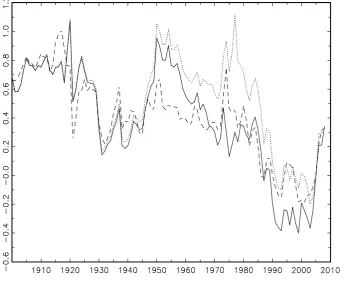
the Grilli-Yang non-fuel weighted aggregate real index (GYCPI).13 _{Figure 2 plots the}

logarithms of these indices over 1900 to 2008. Notably (and as might be expected),

the logarithms of CCPI, CCPI0 and GYCPI appear to move in a relatively consistent

manner over the course of the 20th century. Of course, differences will arise, even

between these similar series. For example, while CCPI and CCPI0are constructed using

variable weights and the HPIM deflator, GYCPI uses constant weights from 1977-79

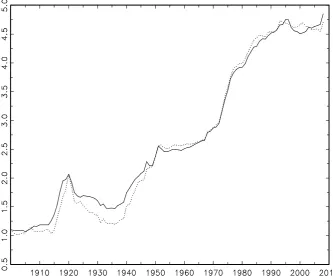
and the MUV deflator. In particular, Figure 3 illustrates how HPIM compares with

the MUV index for the period since 1900, over which the MUV index is available. In

absolute terms the difference is not large and thus is reflected in a very high correlation

coefficient of 0.993. However, and as can be observed in Figure 3, in relative terms there

are a few significant differences, most notably during the period 1914-1945, where the

MUV index is often 25% below our index. As noted by Harveyet al. (2010), this result

suggests that export unit values used to construct the MUV index are potentially biased 12_{In this paper, we employ an extended Harvey} _{et al}_{. (2010) commodity and manufacturing price} dataset that runs from 1650 to 2014. Additionally, we removed gold and silver from the original list of twenty five commodities. There is no clear distinction between monetary gold/silver and commodity gold/silver imports in the US Geological Survey data; this could create a distortion, as, for example, monetary gold and silver were heavily imported during the two world war eras.

(12)

measures of price movements, particularly when long data series are considered.14

3.2 Other historical macroeconomic data

In section 2, it was suggested that macroeconomic variables related to commodity prices

include income, interest rates and supply. Although annual data on quantities traded

for many commodities is only available post-World War 2, longer-run series are available

for income and interest rates. For example, in terms of income, we initially source our

income data, similarly to Erten and Ocampo (2013), from Angus Maddison’s data,

updated recently by the Maddison Project.15 _{From here we obtain (i) World GDP}16

for 1820-2009 (ii) USA GDP from 1820-2009 (iii) Chile GDP from 1870-2009 and (iv)

China from 1950-2009. Of course, the UK became the world’s pre-eminent economy

over the course of the 17th to 19th century and by the early 1800s had the highest per

capita income in the world (see Bolt and Van Zenden, 2013). However, Maddison’s

annual data for UK GDP only goes back to 1800. Recently, Broadberry et al. (2011)

produced a real output series for the UK from 1270 to 1870, and we use these data

from 1650.

Finally, sources of historical interest rate data are more difficult to obtain but the

Bank of England (see Hills et al., 2010) have recently made available annual data on

long-term UK government bonds from 1703 and this is used in our later analysis. 14_Harvey_{et al}_{. (2010) suggest the value added price deflator used by HPIM has three advantages} over export unit values: first, it omits the influence of intermediate products; second, it allows for compositional changes; and third, technological progress is, to some extent, reflected in the deflator.

15_{See http://www.ggdc.net/maddison/maddison-project/home.htm}

(13)

4 Empirical results and discussion

4.1 Commodity price trend function analysis

Table 1 shows the results of applying the order of integration robust trend testtRQF_β (MU)

presented in section 4.1 to the new relative commodity price indices outlined in section

3.17 _{The table also reports estimated growth rates and confidence intervals based on the}

quasi-feasible GLS (Generalized Least Squares) approach of Perron and Yabu (2009a).

Notably, for both new series CCPI and CCPI0 over the full sample, the null of no trend

is rejected in favour of the alternative of a negative trend at the 1% significance level.

This is a striking result, particularly when considering the sample length of the new

commodity indices. The two series, commencing in 1650, have declined subsequently

at an annual average rate of just below 0.9%.

On the other hand, although the three sub-sample series also display negative

growth rates, only the test statistic for the GYCPI series is large enough to reject

the null from 1900 onwards. The inability of the CCPI and CCPI0 series to generate

rejections of the null of no trend is perhaps reflective of their relatively larger variance

over the course of the 20th century, compared with the GYCPI data. Note that testing

against a two-sided alternative (allowing for the possibility of positive trends) does not

lead to any further rejections of the no trend null.

Focusing now on the two ultra-long series (CCPI and CCPI0), it is important to

next consider the possibility that one or more structural breaks have occurred in the

deterministic trend function, as discussed in section 2.3. Table 2 reports results for

the Kejriwal and Perron (2010) sequential order of integration robust procedure for

detecting the number of breaks in level/trend, up to the maximum number permitted

of three. For each step of the sequential procedure, the table reports results for the

FT(l+ 1|l) test, and, if a rejection is obtained in favour of l+ 1 break(s), the estimated

17_The _tRQF

(14)

break date(s) obtained at each stage are also reported. The end result of the procedure

is a finding of evidence (at the 1% significance level) in favour of three breaks in

level/trend for both CCPI and CCPI0. The breaks occur at the dates 1820, 1872/3 and

1946, with the corresponding fitted values at these minimum global SSR dates, i.e. the

fitted values from (6), given by:

CCPI: pt = 2.88−0.0079t

+ 0.34DU1t(1820) + 0.0031DT1t(1820)

−0.37DU2t(1872)−0.0087DT2t(1872)

+ 0.48DU3t(1946)−0.0003DT3t(1946) + ˆut

CCPI0: pt = 2.88−0.0079t

+ 0.34DU1t(1820) + 0.0032DT1t(1820)

−0.39DU2t(1873)−0.0080DT2t(1873)

+ 0.69DU3t(1946)−0.0015DT3t(1946) + ˆut

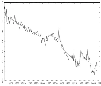
Graphical representations of these results are given in Figures 4 and 5.

The two commodity price indices can therefore be approximately split into four

intertemporal regimes: 1650 to the early 1820s; the early 1820s to the early 1870s;

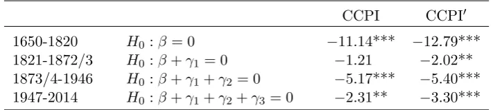
the early 1870s to the mid-1940s; and the mid-1940s to the present day. To ascertain

whether the trends in each of these four regimes are significantly negative, we wish to

test the following hypotheses (based on the model (6)): H0 :β = 0 for the first regime

(1650-1820),H0 :β+γ1 = 0 for the second regime (1821-1872/3),H0 :β+γ1+γ2 = 0 for

the third regime (1873/4-1946), andH0 :β+γ1+γ2+γ3 = 0 for the fourth regime

(1947-2010), in each case against a one sided (lower tailed) alternative. In order to conduct

(15)

we consider a quasi-feasible GLS-based testing approach consistent with the Perron

and Yabu (2009b) approach for testing for a break. The resulting

autocorrelation-corrected t-statistics are then formed in an analogous way to WRQF(T1B) of Perron

and Yabu (2009b), and, conditional on the break dates, follow asymptotic standard

normal distributions under the respective null hypotheses. Table 3 reports the results,

and we find strong evidence in favour of a declining trend in all regimes for CCPI0, and

for CCPI, all regimes apart from 1821-1872, where the trend estimate is negative but

found to be insignificantly different from zero.

The vast majority of work has examined the PS hypothesis over the post-1900

period but we can now additionally comment on its relevance prior to the 20th century.

Strikingly, our results confirm that relative commodity prices present a significant and

downward global trend over almost the entire sample period. With the exception of

the 1821-1872 period, the growth rates of the commodity price indices were found

to decline in the ranges −0.79% to −1.38% per annum for CCPI, and −0.79% to

−1.42% per annum for CCPI0, over the different regimes. It is noticeable that the broadly declining trend paths of the price series are punctuated by structural breaks

in the level and trend; 1820 shows a sharp rise in the level and trend, 1872/3 sees a

sharp fall in level and trend, while 1946 shows a rise in level18_{. This identification of}

changing trend behaviour provides new characterisations of historical price behaviour –

for example, the 19th century terms of trade boom (see Williamson, 2008) is captured

by a local increase in prices during the second regime (i.e. early 1820s to the early

1870s), superimposed on a generic long-run downward trend. Moreover, the results

suggest that the decline in trend has been greater since the early 1870s than at any

(16)

causes behind the modern incarnation of the PS hypothesis therefore appear arguably

stronger than those that existed in the more distant past – we shall return to this later.

4.2 Macroeconomic variables trend function analysis

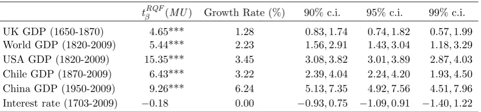
The results of the trend and trend break tests for our macroeconomic series are shown

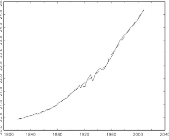
in Tables 4 and 5 respectively.19 Interestingly, UK GDP (plotted in Figure 6) shows a significant and positive trend growth rate of 1.28% per annum over the 1650 to 1870

sample period. Moreover, a positive break in the trend in 1817, captures the UK’s

rising industrial production driven by technological advances in manufacturing and

growth, and closely matches the first break found in our CCPI series.

The US overtook the UK in terms of GDP in the 1870s (see Broadberry and Klein,

2011) and the rest of the industrial core also grew strongly over much of the 19th and

20th century. This is reflected in the growth of World GDP plotted in Figure 7 for

1820-2009. Table 4 shows the trend presents a growth rate of 2.23% per annum whilst

Table 5 shows breaks of a positive sign occur in the trend during the 1870s and 1950s.

Again, these breaks closely match those identified for earlier CCPI series. Overall, it

would appear that since the 1870s, increasing rates of trend economic growth in World

GDP are associated with declining trend rates in relative commodity prices. Both

trends may reflect a latent common factor such as increasing technological innovation.

Of course, since the mid-1990s and over most of the first decade of the 21st century,

commodity prices rose (see Figures 1 and 2). Academics (see, for example, Cuddington

and Jerrett, 2008) and commentators alike asked whether prices were in a positive

growth phase of a supercycle; a medium length cyclical movement with a periodicty

between 20 and 40 years. Explanations for higher prices include the rapid economic

(17)

Figure 8 plots the available Maddison GDP data for China from 1950 .20 Interestingly, China’s path of trend growth broke positively around the late 1970s and has since shown

particularly high growth rates of 7.5% per annum. If this continued, real commodity

prices could remain supported above trend (similar to the mid-19th century) for a

number of years. However, recent price falls occurred during 2014 and are associated

with falling oil prices and concerns around the future economic growth of countries like

China.

Finally, before examining the relationship between commodity prices and

macroe-conomic variables, we note that the interest rate, as one might expect, presents no

trend.

4.3 Stationary VAR analysis

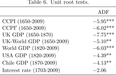
Recent work such as Erten and Ocampo (2013) has tested whether real commodity

prices and income are cointegrated. To assess whether this approach is appropriate,

we first test each series for a unit root. Table 6 presents results of ADF-type unit root

tests that account for the breaks in level/trend that we have previously determined.

Specifically, we conduct the additive outlier unit root t-tests of Perron (1989)

(incor-porating the Perron and Vogelsang (1993) correction), extended appropriately to the

multiple break case, with critical values obtained by simulation of the corresponding

limit distributions, conditioning on the number and timing of breaks in each case. The

lag order is determined using the Schwarz Information Criterion with a maximum of 12

lagged differences. We find evidence in favour of stationarity (around the broken trend

function) for all series except the interest rate. A cointegration approach is therefore

not appropriate, and we proceed to analyse the relationships between the variables

using a stationary VAR analysis, based on the de-trended commodity price and GDP

(18)

interest rate. A stationary VAR(p) of the following form is estimated:

zt=v+A1zt−1+...+Apzt−p+ut, t= 1, ..., T (7)

where zt = (z1t, ..., zkt)0. Following L¨utkepohl (2005), lag lengths are chosen for pairs

of commodity price series21 and GDP, and where data are available, combinations of commodity prices, GDP and interest rates, by comparing the results of a selection of

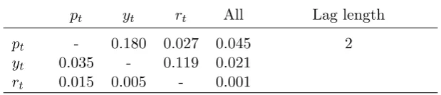
information criteria (IC)22_{. Table 7 shows the results of Granger causality tests, within}

the different VAR frameworks. By way of explanation, consider Panel A which refers

to a VAR(1) of CCPI and a joint UK-World GDP series that covers the entirety of our

sample period. Here the p-value of 0.044 suggests that CCPI Granger causes GDP.

Taken as a whole, the other results in Table 7 confirm that commodity prices appear to

Granger cause income and interest rates, whilst interest rates23 tend to Granger cause prices. Interestingly, these implications hold whether we examine combinations of our

composite commodity price index and US GDP or individual commodity price series

like copper, with GDP from commodity exporting economies like Chile.

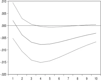
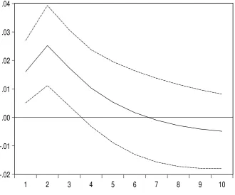
Of course, we might expect shocks to composite commodity prices on US GDP, to

have a different affect to those shocks to copper prices on Chile GDP. Impulse response

functions, show this to be the case, with positive innovations to CCPI leading to a fall

in US GDP (see Figure 9), whilst a similar innovation to the copper price sees a rise

in Chile GDP (see Figure 10). It is notable that innovations to interest rates cause a

fall in commodity prices, whilst innovations to prices lead to a rise in interest rates no

matter what combination of prices and interest rate we observe.

21_{We only show results for CCPI in the multivariate analysis, as the results with CCPI}0_{are similar.}

China is removed from this section of analysis as its GDP data are only available annually from 1950. 22_{Using a maximum lag length of 8 years, we use the Schwarz, Akaike and Hannan-Quinn} Infor-mation Criterion. When the ICs agree, that lag length is selected. When they disagree, the IC that shows the most evidence of Granger causality is displayed

(19)

5 Conclusions

Many developing countries present export earnings that are primary commodity

depen-dent. Therefore, the presence of a secular decline in primary commodity relative prices

as implied by the Prebisch-Singer hypothesis, suggests that unless developing countries

diversify into manufactures and/or services, they will incur long-run economic

stagna-tion. However, as Deaton and Laroque (2003) note, the literature has a relatively

limited understanding of both the causes of the long-run path in relative commodity

prices and any movements around that path. Given the recent availability of relevant

historical data, we suggest a very long-run approach to examine both issues.

First, we suggest that aggregating relative commodity prices over the very

long-run can smooth idiosyncratic effects and provide summary series shaped primarily by

common factors. To this end, this paper constructs new aggregate real commodity price

series from 1650 to 2014. The series are created by combining a new historical dataset

on the export values of 23 commodities, with the individual commodity price dataset

from Harvey et al. (2010). Subsequently, employing multiple break techniques robust

to whether or not each series contains a unit root, it is shown that the trend path of

these series can be partitioned into four regimes (i.e. 1650 to the early 1820s, the early

1820s to the early 1870s, the early 1870s to the mid-1940s, and the mid-1940s to 2014).

A long-run downward trend is estimated in all but the second regime, revealing that

the Prebisch-Singer hypothesis has relevance for the 17th, 18th and 20th centuries at

least. However, it is also shown that the series declined at a slower rate over the 17th

and 18th centuries as compared with the 20th century, suggesting that the economic

forces underlying the hypothesis intensified over this recent period.

Secondly, again employing multiple break techniques, we examine the time series

behaviour of several macroeconomic series over our long sample period. As might be

expected a number of breaks are found and in particular, it is shown that breaks in

(20)

dated analgously to those in the trend of commodity prices. This increasing rate of

trend growth in GDP as the sample increases, coupled with the decreasing rate of trend

growth for commodity prices, suggests a common latent factor such as technological

in-novation may be behind both. Certainly,inter alios, Sachs and McArthur (2002) stress

that technological innovation is a fundamental driver of long-run economic growth.

Thirdly, given recent work has suggested economic activity and interest rates are

related to commodity prices, we model the relationships between our long-run series.

As a precursor to this, the data are initially demeaned and detrended according to the

breaks found. Although income and commodity prices are often modelled as I(1) in

the literature, our residual series are typically found to be I(0) and therefore we adopt

stationary VAR approach. Strikingly, whether we assess large economy GDP like the

US with composite price indices or commodity exporting countries such as Chile and

the real price of its copper exports, there is evidence that commodity prices Granger

cause GDP and interest rates, whilst interest rates Granger cause commodity prices.

There would appear to be several lessons for the present day. For example, it would

appear likely, given our analysis, that the recent loose monetary policy supported higher

commodity prices. However, now that such prices are falling, policymakers should note

the historical asymmetric effect: a GDP boost for commodity importers but a fall for

commodity exporters. The recent slowdown in the growth of BRIC (Brazil, Russia,

India, China) countries appears likely to continue whilst commodity prices remain low.

References

Arango, L.E., Arias, F., Florez, A., 2012. Determinants of Commodity Prices.

Ap-plied Economics 44, 135-145.

Arezki, R., Loungani, P., van der Ploeg, R., Venables, A.J., 2014a. Understanding

(21)

and Finance 42, 1-8.

Arezki, R., Hadri, K., Loungani, P., Rao, Y., 2014b. Testing the Prebisch-Singer

Hypothesis since 1650: Evidence from Panel Techniques that Allow for Mulitple

Breaks. Journal of International Money and Finance 42, 208-223.

Bairoch, P., Etemad, B., 1985. Commodity Structure in Third World Exports

1830-1937. Geneva: Librairie Droz.

Blattman, C., Hwang, J., Williamson, J.G., 2007. Winners and Losers in the

Com-modity Lottery: The Impact of Terms of Trade Growth and Volatility in the

Periphery 1870-1939. Journal of Development Economics 82, 156-179.

Bolt, J., van Zenden, J.L, 2013.The First Update of the Maddison Project:

Re-Estimating Growth Before 1820. Maddison-Project Working Paper WP-4.

Borensztein, E., Reinhart, C.M., 1994. The macroeconomic determinants of

commod-ity prices. IMF Staff Papers 41, 236-261.

Broadberry, S.N., Campbell, B.N., Klein, A., Overton, M., van Leeuwen, B. 2011.

British Economic Growth, 1270-1870: An Output-Based Approach. Department

of Economics, University of Kent, Working Paper Series Studies in Economics

No.1203.

Broadberry, S.N., Klein, A., 2012. Aggregate and Per Capita GDP in Europe,

1870-2000: Continental, Regional and National Data with Changing Boundaries.

Scan-dinavian Economic History Review 60, 79-107.

Chu, K., Morrison, T., 1986. World non-oil primary commodity markets: a

medium-term framework for analysis. IMF Staff Papers 33, 139-184.

Cuddington, J. and Jerrett, D., 2008. Super Cycles in Metals Prices? IMF Staff

(22)

Deaton, A. 1999. Commodity Prices and Growth in Africa. Journal of Economic

Perspectives 13, 23-40.

Deaton, A., Laroque, G., 2003. A Model of Commodity Prices after Sir Arthur Lewis.

Journal of Development Economics 71, 289-310.

Erten, B., Ocampo, J.A., 2013. Super Cycles of Commodity Prices Since the

Mid-Nineteenth Century. World Development 44, 14-30.

Frankel, J., 2006. The effect of monetary policy on real commodity prices. NBER

Working Paper No. 12713.

Ghoshray, A., 2011. A Reexamination of Trends in Primary Commodity Prices.

Journal of Development Economics 95, 242-251.

Gilbert, C.L., 1989. The impact of exchange rates and developing country debt on

commodity prices. Economic Journal 99, 773-784.

Grilli, R.E., Yang, M.C. 1988. Commodity Prices, Manufactured Goods Prices, and

the Terms of Trade of Developing Countries. World Bank Economic Review 2,

1-48.

Harvey, D.I., Kellard, N.M., Madsen, J.B., Wohar, M.E. 2010. The Prebisch-Singer

Hypothesis: Four Centuries of Evidence. Review of Economics and Statistics 92,

367-377.

Harvey, D.I., Leybourne, S.J., Taylor, A.M.R., 2007. A Simple, Robust and Powerful

Test of the Trend Hypothesis. Journal of Econometrics 141, 1302-1330.

Hills, S., Thomas, R., Dimsdale, N., 2010. The UK recession in context what do

(23)

Kejriwal, M., Perron, P., 2010. A Sequential Procedure to Determine the Number of

Breaks in Trend with an Integrated or Stationary Noise Component. Journal of

Time Series Analysis 31, 305-332.

Kellard, N., Wohar, M.E., 2006. On the Prevalence of Trends in Primary Commodity

Prices. Journal of Development Economics 79, 146-167.

L¨utkepohl, H., 2005. New introduction to multiple time series analysis. Springer.

Miller, G., Urdinola, B.P., 2010. Cyclicality, Mortality, and the Value of Time: The

Case of Coffee Price Fluctuations and Child Survival in Colombia. Journal of

Political Economy 118, 113-155.

Perron, P., 1989. The Great Crash, the Oil Price Shock, and the Unit Root

Hypoth-esis. Econometrica 57, 1361-1401.

Perron, P., Vogelsang, T.J., 1993. The Great Crash, the Oil Price Shock, and the

Unit Root Hypothesis: Erratum. Econometrica 61, 248-249.

Perron, P. and Yabu, T., 2009a. Estimating Deterministic Trends with an Integrated

or Stationary Noise Component. Journal of Econometrics 151, 56-69.

Perron, P. and Yabu, T., 2009b. Testing for Shifts in Trend With an Integrated or

Stationary Noise Component. Journal of Business and Economic Statistics 27,

369-396.

Poelhekke, S., van der Ploeg, R., 2009. Volatility and the Natural Resource Curse.

Oxford Economic Papers 61, 727-760.

Pongou, R., Salomon, A., Ezzati, M., 2006. Health Impacts of Macroeconomic Crises

and Policies: Determinants of Variation in Childhood Malnutrition Trends in

(24)

Prebisch, R., 1950. The Economic Development of Latin America and its Principal

Problems. Economic Bulletin for Latin America 7, 1-12.

Sachs, J. D., McArthur, J. W., 2002. Technological Advance and Long-Term

Eco-nomic Growth in Asia. In: Chong-En Bai, Chi-Wa Yuen (Eds.), Technology and

the New Economy. Cambridge, MA: MIT Press, pp. 157-185.

Sapsford, D., 1985. The Statistical Debate on the Net Terms of Trade Between

Primary Commodities and Manufacturers: A Comment and Some Additional

Evidence. Economic Journal 95, 781-788.

Sapsford, D.P., Sarkar, P., Singer, H.W., 1992. The Prebisch-Singer Terms of Trade

Controversy Revisited. Journal of International Development 4, 315-332.

Singer, H., 1950. The Distribution of Gains Between Investing and Borrowing

Coun-tries. American Economic Review (Papers and Proceedings) 40, 473-485.

Spraos, J., 1980. The Statistical Debate on the Net Barter Terms of Trade. Economic

Journal 90, 107-128.

Sumner, D.A., 2009. Recent Commodity Price Movements in Historical Perspective.

American Journal of Agricultural Economics 91, 1250-1256.

Thirwall, A.P., Bergevin, J., 1985. Trends, Cycles, and Asymmetry in Terms of Trade.

World Development 13, 805-817.

Williamson, J.G., 2008. Globalization and the Great Divergence: Terms of Trade

Booms, Volatility and the Poor Periphery, 1782–1913. European Review of

(25)

6 Data Appendix

6.1 Commodity data sources

The weighted average commodity price indices are constructed using export values

from developing countries as weights, over the period 1830-2014. The sources used are

as follows:

1. 1830-1937. Principle source (for commodities Banana, Beef, Cocoa, Coffee,

Cot-ton, Hides, Jute, Oil, Pig Iron, Sugar, Tea, Tobacco, Wheat and Wool):

Com-modity Structure of Third World Exports 1830-1937, Paul Bairoch and Bouda

Etemad, Centre of International Economic History, University of Geneva.

2. 1830-1937. Secondary sources (for commodities Aluminum, Coal, Copper, Lamb,

Lead, Nickel, Rice, Tin and Zinc); imports to developed countries are used as a

proxy for exports from developing countries:

(a) US Geological Survey;

(b) Statistical Yearbook of Canada, 1899;

(c) Annuaire Statistique de la France, Vol. 19, 1899;

(d) Entwicklung und Strukturwandlungen des Englischen Außenhandels von

1700 bis zur Gegenwart, Werner Schlote, Probleme der Weltwirtschaft, Jena

Fischer, 1938;

(e) Statistical Abstract for the United Kingdom in Each of the Last Fifteen

Years from 1871 to 1885, HMSO, 1986.

3. 1938-2014. All data from 1962-2014 are obtained from the from the Comtrade

database, http://comtrade.un.org/data/. Trade weights between 1938 and 1961

(26)

6.2 Composite commodity price index construction

When constructing the CCPI, the following steps have been followed. First, the

com-modity price index (CPI) is calculated usingPN_i₌₁witpit, wherewitand pitrespectively

represent the weight and price of the ith commodity in a particular year t. If prices

and weights are available forN −1 commodities in the first t= 1, ..., xyears and then for N commodities in the next t = x+ 1, ..., y years, individual CPI series are first

constructed for each period t = 1, ..., x+ 1 and t = x+ 1, ..., y using data on N −1 and N commodities, respectively. Next, denote by w_i,xN−₊₁1 and wN

i,x+1 the weights

em-ployed in these two schemes for the overlapping year t =x+ 1. Then, using the ratio

PN

i=1wNi,x+1pi,x+1/PN

−1

i=1 w

N−1

i,x+1pi,x+1, the aggregate series is created by multiplying the

ratio by the individual CPI values for thet= 1, ..., xperiod and splicing the individual

series together to assemble the CCPI.

Several benchmark years, namely 1830, 1860, 1900, 1912, 1928, 1937 and 1962

onwards are used to calculate the weights of commodities. Specifically, exports of

commodities from the commodity-dependent price-taking economies (the periphery24₎

are used as weights. To be clear, the export value of the ith commodity is divided by

the total export value of all selected N commodities in year t to get the weight, wit,

of the ith commodity in year t. The periphery consists of Asia (excluding Russia),

Africa and South America. The benchmark dates are predominantly dictated by data

availability; in particular, data on commodity exports are not available before 1830

on a world scale and it is doubtful that the scant import data that are available for a

couple of industrialized countries before 1830 are representative of commodity exports

for the periphery. In terms of composition of traded commodities there has been a

marked change over time. Sugar, textile fibres, coffee, tea and cocoa were the main

(27)

energy and metals have recently become the dominant commodities in world trade.

The benchmark years are subsequently linearly interpolated to get weighted series

for each commodity on an annual basis. Specifically, interpolation is applied between

the benchmark years from 1830 to 1962; to complete the series, 1830 weights are used

before 1830 and annual weights are used after 1962 until 2014. Although weights before

1830 are kept constant due to unavailability of data, the weights of commodities have

been calculated such that their sum remains 100 in each year. For years where price

data are unavailable for a few commodities, weights for those commodities in those

years are set to zero under the assumption that a commodity has no value or weight

when the price is zero. This leads to the construction of the CCPI covering a 365 year

(28)

[image:28.595.78.524.92.254.2]

Table 1. Tests for a negative trend and estimated growth rates.

Panel A. 1650-2014

t_βRQF(MU) Growth Rate (%) 90% c.i. 95% c.i. 99% c.i.

CCPI −17.45*** −0.88 −0.96,−0.80 −0.98,−0.78 −1.01,−0.75 CCPI0 −17.06*** −0.84 −0.92,−0.76 −0.94,−0.74 −0.97,−0.71

Panel B. 1900-2008

CCPI −0.25 −0.32 −2.40, +1.77 −2.79, +2.16 −3.56, +2.93 CCPI0 −0.37 −0.35 −1.87, +1.18 −2.16, +1.47 −2.73, +2.03 GYCPI −4.08*** −0.58 −0.81,−0.34 −0.85,−0.30 −0.94,−0.21

[image:28.595.69.536.353.437.2]

Note: *** denotes rejection at the 1% significance level.

Table 2. Sequential tests for multiple breaks in level/trend.

CCPI CCPI0

FT(l+ 1|l) Estimated break date(s) FT(l+ 1|l) Estimated break date(s)

FT(1|0 ) 9.17*** 1881 8.88*** 1882

FT(2|1 ) 9.51*** 1823, 1946 8.81*** 1823, 1946

FT(3|2 ) 15.71*** 1820, 1872, 1946 15.64*** 1820, 1873, 1946

Table 3. Tests for a negative trend in sub-sample regimes.

CCPI CCPI0

1650-1820 H0:β = 0 −11.14*** −12.79*** 1821-1872/3 H0:β+γ1 = 0 −1.21 −2.02** 1873/4-1946 H0:β+γ1+γ2= 0 −5.17*** −5.40*** 1947-2014 H0:β+γ1+γ2+γ3 = 0 −2.31** −3.30***

[image:28.595.125.481.536.616.2]

(29)

[image:29.595.59.553.92.207.2]

Table 4. Tests for a trend and estimated growth rates.

UK GDP (1650-1870) 4.65*** 1.28 0.83, 1.74 0.74, 1.82 0.57, 1.99 World GDP (1820-2009) 5.44*** 2.23 1.56, 2.91 1.43, 3.04 1.18, 3.29 USA GDP (1820-2009) 15.35*** 3.45 3.08, 3.82 3.01, 3.89 2.87, 4.03 Chile GDP (1870-2009) 6.43*** 3.22 2.39, 4.04 2.24, 4.20 1.93, 4.50 China GDP (1950-2009) 9.26*** 6.24 5.13, 7.35 4.92, 7.56 4.51, 7.96 Interest rate (1703-2009) −0.18 0.00 −0.93, 0.75 −1.09, 0.91 −1.40, 1.22

Table 5. Sequential tests for multiple breaks in level/trend.

UK (1650-1870)

FT(l+ 1|l) Estimated break date(s)

FT(1|0 ) 31.04*** 1790

FT(2|1 ) 69.10*** 1773, 1817

World (1820-2009)

FT(1|0 ) 15.13*** 1933

FT(2|1 ) 23.73*** 1872, 1955

USA (1820-2009)

FT(1|0 ) 11.53*** 1913

FT(2|1 ) 8.45*** 1930, 1945

Chile (1870-2009)

FT(1|0 ) 3.70** 1930

China (1950-2009)

FT(1|0 ) 12.07*** 1976

[image:29.595.165.442.308.627.2]

(30)

[image:30.595.184.421.79.231.2]

Table 6. Unit root tests.

ADF

CCPI (1650-2009) −5.95*** CCPI0 (1650-2009) −6.02*** UK GDP (1650-1870) −7.75*** UK-World GDP (1650-2009) −5.10** World GDP (1820-2009) −6.03*** USA GDP (1820-2009) −4.39** Chile GDP (1870-2009) −4.13** Interest rate (1703-2009) −2.06

Note: *,** and *** denote rejection at the 10%, 5% and 1% significance levels respectively. The UK-World GDP series is an index of UK

(31)

[image:31.595.148.458.594.661.2]

Table 7. VAR Granger causality tests.

Panel A. CCPI and UK-World GDP (1650-2009)

pt yt rt All Lag length

pt - 0.900 - 0.900 1

yt 0.044 - - 0.044

rt - - -

-Panel B. CCPI, UK-World GDP, Interest Rates (1703-2009)

pt - 0.171 0.107 0.093 1

yt 0.113 - 0.741 0.274