Clustering-based redshift estimation: application to VIPERS/CFHTLS
V. Scottez,
1‹Y. Mellier,
1,2B. R. Granett,
3T. Moutard,
4M. Kilbinger,
1,2M. Scodeggio,
5B. Garilli,
5M. Bolzonella,
6S. de la Torre,
4L. Guzzo,
3U. Abbas,
7C. Adami,
4S. Arnouts,
4D. Bottini,
5E. Branchini,
8,9,10A. Cappi,
6,11O. Cucciati,
12,6I. Davidzon,
4,6A. Fritz,
5P. Franzetti,
5A. Iovino,
3J. Krywult,
13V. Le Brun,
4O. Le F`evre,
4D. Maccagni,
5K. Małek,
14F. Marulli,
12,15,6M. Polletta,
5A. Pollo,
16,14L. A. M. Tasca,
4R. Tojeiro,
17D. Vergani,
18,6A. Zanichelli,
19J. Bel,
20J. Coupon,
21G. De Lucia,
22O. Ilbert,
4H. J. McCracken
1and L. Moscardini
6,12,151Institut d’Astrophysique de Paris, UMR7095 CNRS, Universit´e Pierre and Marie Curie, 98 bis boulevard Arago, F-75014 Paris, France 2CEA/Irfu/SAp Saclay, Laboratoire AIM, F-91191 Gif-sur-Yvette, France
3INAF – Osservatorio Astronomico di Brera, Via Brera 28, 20122 Milano, via E. Bianchi 46, I-23807 Merate, Italy 4Aix Marseille Universit´e, CNRS, LAM (Laboratoire d’Astrophysique de Marseille) UMR 7326, F-13388 Marseille, France 5INAF – Istituto di Astrofisica Spaziale e Fisica Cosmica Milano, via Bassini 15, I-20133 Milano, Italy
6INAF – Osservatorio Astronomico di Bologna, via Ranzani 1, I-40127, Bologna, Italy 7INAF – Osservatorio Astronomico di Torino, I-10025 Pino Torinese, Italy
8Dipartimento di Matematica e Fisica, Universit`a degli Studi Roma Tre, via della Vasca Navale 84, I-00146 Roma, Italy 9INFN, Sezione di Roma Tre, via della Vasca Navale 84, I-00146 Roma, Italy
10INAF – Osservatorio Astronomico di Roma, via Frascati 33, I-00040 Monte Porzio Catone (RM), Italy
11Laboratoire Lagrange, UMR7293, Universit´e de Nice Sophia Antipolis, CNRS, Observatoire de la Cˆote d’Azur, F-06300 Nice, France 12Dipartimento di Fisica e Astronomia – Alma Mater Studiorum Universit`a di Bologna, viale Berti Pichat 6/2, I-40127 Bologna, Italy 13Institute of Physics, Jan Kochanowski University, ul. Swietokrzyska 15, PL-25-406 Kielce, Poland
14National Centre for Nuclear Research, ul. Hoza 69, PL-00-681 Warszawa, Poland 15INFN, Sezione di Bologna, viale Berti Pichat 6/2, I-40127 Bologna, Italy
16Astronomical Observatory of the Jagiellonian University, Orla 171, PL-30-001 Cracow, Poland
17Institute of Cosmology and Gravitation, Dennis Sciama Building, University of Portsmouth, Burnaby Road, Portsmouth PO1 3FX, UK 18INAF – Istituto di Astrofisica Spaziale e Fisica Cosmica Bologna, via Gobetti 101, I-40129 Bologna, Italy
19INAF – Istituto di Radioastronomia, via Gobetti 101, I-40129 Bologna, Italy 20Aix Marseille Universit´e, CNRS, CPT, UMR 7332, F-13288 Marseille, France
21Astronomical Observatory of the University of Geneva, ch. d’Ecogia 16, CH-1290 Versoix, Switzerland 22INAF – Osservatorio Astronomico di Trieste, via G. B. Tiepolo 11, I-34143 Trieste, Italy
Accepted 2016 June 10. Received 2016 June 9; in original form 2016 May 17
A B S T R A C T
We explore the accuracy of the clustering-based redshift estimation proposed by M´enard et al. when applied to VIMOS Public Extragalactic Redshift Survey (VIPERS) and Canada– France–Hawaii Telescope Legacy Survey (CFHTLS) real data. This method enables us to reconstruct redshift distributions from measurement of the angular clustering of objects using a set of secure spectroscopic redshifts. We use state-of-the-art spectroscopic measurements
withiAB<22.5 from the VIPERS as reference population to infer the redshift distribution of
galaxies from the CFHTLS T0007 release. VIPERS provides a nearly representative sample
to a flux limit of iAB<22.5 at a redshift of >0.5 which allows us to test the accuracy of
the clustering-based redshift distributions. We show that this method enables us to reproduce the true mean colour–redshift relation when both populations have the same magnitude limit. We also show that this technique allows the inference of redshift distributions for a population fainter than the reference and we give an estimate of the colour–redshift mapping in this case. This last point is of great interest for future large-redshift surveys which require a complete faint spectroscopic sample.
Key words: methods: data analysis – surveys – clustering – galaxies: distances and redshifts.
E-mail:[email protected]
1 I N T R O D U C T I O N
Large future redshift surveys like the ESAEuclid space mission (Laureijs et al.2011; Amendola et al.2013) aim to probe dark en-ergy with unprecedented accuracy. Many of the cosmological mea-surements to be performed with these surveys – e.g. tomographic weak lensing, tomographic clustering – will require extremely well-characterized redshift distributions (Albrecht et al.2006; Huterer et al.2006; Ma, Hu & Huterer2006; Thomas et al.2011).
Since it is impractical to measure spectroscopic redshifts for hundreds of millions of galaxies – especially extremely faint ones – these experiments are largely dependent upon photometric redshifts: i.e. estimates of the redshifts of objects based only on flux infor-mation obtained through broad-band filters. Photos-z also require large spectroscopic samples both for the calibration of empirical methods (Connolly et al.1995) and the building of representative template libraries for template-fitting techniques (Coleman et al. 1980). However, current and future spectroscopic surveys will be highly incomplete due to selection biases dependent on redshift and galaxy properties (Cooper et al.2006). Because of this, along with the catastrophic photometric errors that can occur at a significant (∼1 per cent) rate (Sun et al.2009; Bernstein & Huterer2010), pho-tometric redshifts are not sufficiently precise. If future dark energy experiments have to reach their goals, it is necessary to develop a method to infer, at least, the redshift distribution with high precision. Current projections for cosmic shear measurements estimate that the true mean redshift of objects in each photo-z bin must be known to better than∼0.002(1+z) (Knox, Song & Zhan2006; Zhan2006; Zhan & Knox2006) with stringent requirements on the fraction of unconstrained catastrophic outliers (Hearin et al.2010) while the width of the bin must be known to∼0.003(1+z). Newman et al. (2015) investigated the spectroscopic needs for dark energy imaging experiments and insisted on the extremely high (∼99.9 per cent) completeness required for calibration techniques.
The idea of measuring redshift distributions using the apparent clustering of objects on the sky is not new. It was first developed by Seldner & Peebles (1979), Phillipps & Shanks (1987) and Landy, Szalay & Koo (1996). This was practically forgotten mainly due to the rise of photometric redshifts. To face the challenges of future and ongoing dark energy imaging experiments, Newman (2008), Matthews & Newman (2010) and Matthews & Newman (2012) re-applied this method on simulations, while McQuinn & White (2013) proposed an optimal estimator for such a measurement. In this paper, we explore the clustering-based redshift estimation, i.e cluster-z, via a local (i.e. within few Mpc) approach introduced by M´enard et al. (2013, hereafterM13), validated with simulations by Schmidt et al. (2013) and compared to spectroscopic redshift at limiting magnitudermodel<19 by Rahman et al. (2015, hereafter
R15). Recently, Schmidt et al. (2015) applied this technique to continuous fields by inferring the redshift distribution of the cosmic infrared background while Rahman et al. (2016a) and Rahman et al. (2016b) explored this method in near-infrared using Two Micron All Sky Survey Extended and Point Source Catalogues as well as the Sloan Digital Sky Survey Photometric Galaxies. This work aims to explore the strength of cluster-z at fainter magnitudeiAB<22.5
using real data similar to what will be available withEuclidin term of filters and observational strategy and demonstrate our ability to recover the redshift distribution of an unknown sample with 22.5< iAB<23 when the reference sample used for calibration has only iAB<22.5.
This paper is organized as follows. In Section 2, we review the clustering-based redshift formalism, while the data used in this work
are described in Section 3. Then in Section 4, we show our ability to measure the clustering redshift distribution using a tomographic photo-z approach. We also show that this method allows the estima-tion of redshift distribuestima-tion when the sample of unknown redshift is fainter than the reference one. Finally, we free cluster-z from the use of photo-z in Section 5 by selecting subsamples in colour-space and we explore in this case the reconstruction of the colour–redshift mapping for faint objects. Conclusions are presented in Section 6.
2 C L U S T E R I N G - B A S E D R E D S H I F T: F O R M A L I S M
The method used in this paper is based on the work ofM13and R15. We refer the reader to those papers for more details. In this section, we briefly review the formalism.
The key point is that correlated galaxies are at the same location in redshift and on the sky. Sources at different redshift are uncor-related. This clustering information is encoded into the two-point correlation function as an excess probability – compared to a ran-dom distribution – to find two objects close together. This is valid in 3D and, by projection, on the sky. Using a reference sample of secure spectroscopic redshifts – and by looking at the galaxy cluster scale – it is then possible to extract the excess probability of finding a population of galaxies at a given redshift. Obviously, the reference population and the unknown one – for which angular positions are known but redshifts are not – have to overlap on the sky.
The mean surface density of unknown objects at a distanceθ from a reference one which is at a redshiftz, is
ur(θ, z)=R[1+ωur(θ, z)], (1)
whereRis the random surface density of the unknown sample
and ωur(θ, z) is the two-point angular cross-correlation function
between the two samples. Then, one can define the integrated cross-correlation function as
¯
ωur(z)=
θmax
θmin
dθ W(θ)ωur(θ, z), (2)
where the range covered byθvaries with redshift and corresponds to physical distances from few hundred kiloparsecs to several mega-parsecs. Here we worked within a [0.2, 6] Mpc annulus.W(θ) is a weight function –∝θ−0.8– aimed at optimising the overall S/N
and whose integral is normalized to unity. This integrated cross-correlation function represents the excess probability, with respect to a Poisson distribution, to find an object of the unknown sample at an angular distance betweenθminandθmaxfrom a generic object
of the reference sample at redshiftz.
One can also write this quantity as a function of the redshift selection function of sample i∈ {u, r}, dNi/dz, as well as the
galaxy-dark matter biases, ¯bi(z), and the dark matter correlation
function, ¯ωm(z):
¯
ωur=
dz dNu
dz (z) dNr
dz(z) ¯bu(z) ¯br(z) ¯ωm(z). (3)
Applying the narrow sample approximation for the reference sample
dNr/dz=NrδD(z−z) – withδDthe Dirac delta function – we can
then simply invert the previous integral and obtain:
dNu
dz (z)∝ω¯ur(z)×
1 ¯
bu(z)
ׯ 1
br(z) ¯ωm(z)
, (4)
where ¯ωur(z) can be directly measured in data, ¯br(z) can be measured
in the reference sample, ¯ωm(z) is given by the cosmology and ¯bu(z)
Considering a narrow redshift distribution for the unknown sam-ple, we can neglect the variation of its galaxy-dark matter bias with respect to the variation of the number of objects:
d log dNu/dz
dz
d log ¯bu
dz , (5)
we obtain:
dNu
dz (z)∝ω¯ur(z)
1 ¯
br(z) ¯ωm(z)
. (6)
As in equation (5), we can neglect the redshift variation of√ω¯m
with respect to dNr/dz:
d log dNr/dz
dz
d log √ω¯m
dz . (7)
Thus, introducing the clustering amplitude of the reference sample, βr(z), we can write:
βr(z)=
¯
ωrr(z)
¯
ωrr(z0)
∝ b¯r(z)
¯
br(z0)
. (8)
Note that we can defineβu(z) in the same way. As explained in
R15, one should note that this quantity is different from the linear galaxy bias which is usually defined only on large scales for which the galaxy and dark matter density fields are, on average, linearly related. This bias definition includes contributions from small scales where the galaxy and matter fields are non-linearly related. We can then rewrite a model-independent version of equation (6) and we obtain:
dNu
dz (z)∝ω¯ur(z)/βr(z). (9)
Finally, the redshift distribution is normalized to the number of objects in the unknown sample through
dzdNu/dz=Nu. (10)
It is important to realize that to be able to write and use equation (9), we have to select unknown samples with relatively small redshift distributions to have ¯bu(z) orβu(z) slowly varying with redshift. The
ability of selecting subsamples with narrow redshift distributions is quite important to consider: dβu/dz=0.
To directly measure the integrated cross-correlation function, we can simply use the Davis & Peebles (1983) estimator:
¯
ωur(z)=
urz
R
−1. (11)
The error in the measurement is then estimated through Poisson statistic and is given by
σ2
¯
ω=
¯
ω+1
√ Nur 2 + ¯
ω+1
√
NR
2
, (12)
whereNuris the neighbours number of unknown objects over [θmin,
θmax] around reference galaxies andNRis the corresponding number
[image:3.595.307.546.55.268.2]of neighbours for a random distribution.
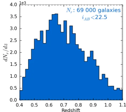
Figure 1. The redshift distribution of the reference sample built from VIPERS data withiAB<22.5 and assuming a bin widthδz=0.02.
3 DATA A N A LY S I S
3.1 The data sets
3.1.1 VIPERS: reference sample
The VIMOS Public Extragalactic Redshift Survey (VIPERS;1
Guzzo et al.2014) is an ongoing spectroscopic survey whose aim is to map the detailed spatial distribution of galaxies. The survey is made of two distinct fields inside the Canada–France–Hawaii Telescope Legacy Survey (CFHTLS) W1 and W4 fields. The total survey area is 24 deg2. VIPERS spectra are the results of 440h of
observation at the Very Large Telescope (VLT) in Chile. Galaxies were selected to havez >0.4 using the following colour criteria:
(r−i)>0.5(u−g) OR (r−i)>0.7. (13) The 1σrandom error in the measured VIPERS redshift is:σz=
0.000 47(1+z).
Our reference sample is made from a selection of VIPERS objects in two separate fields, W1 and W4, outside CFHTLS masks and with secure spectroscopic redshifts (CL>95 per cent) corresponding to flags: 2, 3, 4 and 9 inside the redshift range [0.4, 1.1]. The resulting reference sample is composed of Nr ∼69 000 galaxies with iAB
<22.5 over an area of∼24 deg2. It corresponds to the reference
population used in all the analysis presented in this paper. Its redshift distribution is shown in Fig.1.
3.1.2 CFHTLS: unknown sample
The CFHTLS2-Wide includes four fields labelled W1, W2, W3 and
W4. Complete documentation of the CFHTLS-T0007 release can be found at the Canada–France–Hawaii Telescope (CFHT)3site. In
summary, the CFHTLS-Wide is a five-band survey of intermediate depth. It consists of 171 MegaCam deep pointings (of 1 deg2each)
1http://vipers.inaf.it
which, as a consequence of overlaps, consists of a total of∼155 deg2
in four independent contiguous patches, reaching a 80 per cent com-pleteness limit in AB ofu∗=25.2,g=25.5,r=25.0,i=24.8, z=23.9 for point sources.
In this work, we focused on the W1 and W4 fields in common with VIPERS and used the magnitudes from the VIPERS Multi-Lambda Survey (Moutard et al. 2016a) which is based on the CFHTLS-T0007 photometry. We selected all galaxies in the same region of the sky covered by VIPERS and which are outside CFHTLS masks resulting in a sample of∼570 000 galaxies over∼24 deg2. Since
we use a sample of VIPERS galaxies in the redshift range 0.4<
z <1.1, we will not be able to measure any signal outside this
interval. Unknown objects outside this range will bias the overall redshift distribution, since it is normalized to the total number of unknown galaxies following equation (10). To reduce this problem, we selected objects with a photometric redshift matching the range [0.5, 1] in redshift. Considering the number of photometric sources at the edges and the photometric redshift accuracy, we can expect to have less than 1 per cent of objects outside the redshift range covered by the reference sample. The resulting population corresponds to the parent unknown sample. This parent sample is then divided into two samples: a bright sample with iAB < 22.5 chosen to match
the magnitude limit of the reference population from VIPERS; and a faint sample whose galaxies have magnitudes 22.5<iAB<23.
These are the samples for which we recover the redshift distributions in this paper.
3.1.3 Reference clustering amplitude measurement
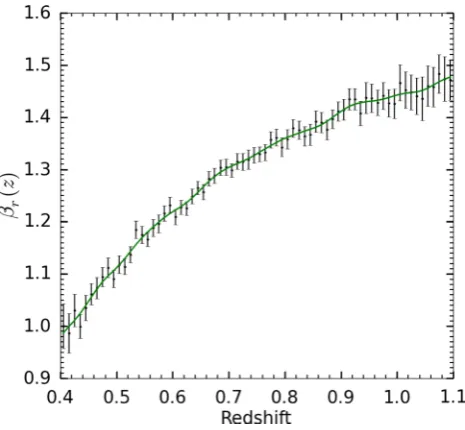
As previously seen in Section 2, the determination of a clustering redshift distribution requires the knowledge of the evolution with redshift of the clustering amplitude of the reference population, βr(z). This quantity can be directly measured using equation (8)
and is shown in Fig.2. We also show a smoothed version obtained by convolving the binned measurements with a Hann filter of width z=0.02. Since we are only interested in the relative variation ofβr(z) – see equations (9) and (10) – we chose to normalize this
Figure 2. Clustering amplitude evolution of the reference sample normal-ized to 1 atz0=0.4. The solid line is the smoothed version used in this paper.
quantity to unity atz0 = 0.4. This figure shows an increase of
∼40 per cent of the clustering amplitude between redshift 0.5 and 1.1 which is in agreement with the analysis performed by Marulli et al. (2013).
4 T O M O G R A P H I C S A M P L I N G
As seen in Section 2, reducing the variation ofβu(z) is a key point of
this method. In this section, we aim at demonstrating our ability to measure the redshift distribution. To reduce the variation ofβu(z),
we choose to work with tomographic subsamples of the unknown population. One can then consider: dβu/dz=0, for each of these
subsamples. The tomography is done by selecting objects using their photometric redshifts based on the marginalization over the redshift of all the models (ZMLin Lephare).
4.1 Photometric redshifts estimation
The photometric redshifts used in this paper come from the VIPERS-MLS and are described in Moutard et al. (2016a). The photometry combines optical data from the CFHTLS-T0007 with near-infrared data (limited atKsAB<22). The authors have used
ISO magnitudes that provide the best estimate of galaxy colour and corrected them for a mean difference between ISO and AUTO mag-nitudes (over theg,r,iandKsbands). This was done in order to recover a good approximation of the galaxy total flux while keeping the best determination of the galaxy colours. In our case, this re-calibration is important since it leads to a smoother surface density fluctuation from tile to tile.
4.2 Magnitude limit for both samples:i<22.5
We selected objects withiAB <22.5 in the unknown population.
The resulting sample containsNu∼203 000 galaxies.
We split them into 68 tomographic subsamples of 3000 objects each. Thus, we measure the integrated cross-correlation from few kpcs to several Mpcs in reference slices of widthδz=0.02.
Fig. 3shows the recovered clustering redshift distribution for a particular tomographic bin selected using the photometric red-shift. We also show the redshift distribution obtained when using photo-z Probability Distribution Functions (PDFs). This PDF is ob-tained by stacking individual PDFs defined as a Gaussian:G(zphot,
σ=zphot,max−zphot,min), wherezphot,min/maxare the 1σlower/upper
limit, respectively. This plot shows the ability of reconstructing the redshift distribution with the clustering method. Recovered distri-butions (black dots) are significantly narrower that the photo-z PDF (dashed green) and consistent with the distribution of spectroscopic VIPERS galaxies (in blue) selected on their photometric redshift to match the selected tomographic bin.
Note that this is not a rigorous comparison since the spectroscopic sources show in blue are not exactly the same objects considered in the unknown sample. Moreover, since there are only few objects in this distribution, one can only compare the statistical properties which are expected to be similar. All distributions are normalized to unity.
In the same way, we measured the clustering redshifts distribu-tions for all the 68 tomographic subsamples. The results of these 68×35=2 380 measurements of ¯ωurare translated into redshift
distributions following equation (9).
[image:4.595.47.280.482.697.2]Figure 3. Example of the cluster-z distribution (black) obtained from equa-tion (9) for a tomographic sample selected using the photo-z (green line). The dashed green line shows the redshift distribution obtained when sum-ming the photo-z PDFs. The blue line shows the spectroscopic redshift distribution with Poisson error bar of the VIPERS sources selected using their photometric redshifts to match the tomographic bin.
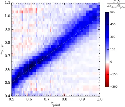
the corresponding redshift distributions in the (zclust;zphot) plane
and illustrates the global agreement between cluster and photo-z. Negative values correspond to stochastic density fluctuations and are not statistically significant.
To compare these two measurements in a more quantitative way, we compute the accuracy of the estimate of the mean redshift of a distribution as:σ =σ ¯z/(1+¯zspec), where ¯z= |¯zclust/phot−z¯spec|
is the difference between the mean clustering redshift and the mean spectroscopic redshift of a distribution.
We use the normalized median absolute deviation to estimate the accuracy as previously defined:
σ ¯z=1.48×median(|z¯clust/phot−z¯spec|), (14)
where the mean redshifts are computed as
¯
z= 1
dN/dz
i
ziddzNi . (15)
For each cluster-z distribution, we show on the top panel of Fig.5 the difference ¯zclust/phot−z¯spec. We see that cluster-z and photo-z are
in relatively good agreement. This figure demonstrates the ability of cluster-z to infer redshift distributions of a sample for which photometric redshifts are known and can be used to reduce the variation ofβu(z) by selected subsamples localized in redshift.
[image:5.595.87.507.346.705.2]Figure 5. Top panel: histograms showing the distribution of the difference between the mean of the clustering/photometric redshift distribution and the mean of the spectroscopic redshift distribution: ¯zclust/phot−z¯spec(black and dashed green lines, respectively). Cluster-z measurements were made con-sidering dβu/dz=0. Bottom panel: same quantities as in the top panel but the cluster-z measurements were performed considering a linear evolution for the clustering amplitude of the unknown population: dβu/dz=1.
The lower panel shows the ¯zclust/phot−z¯specresiduals when
con-sidering a linear evolution of the unknown clustering amplitude dβu/dz= 1 instead of a constant evolution followingR15. This
tomographic sampling approach does not allow us to estimateβu(z)
using photo-z due to the thickness of the selected bins. This will be done in the colour sampling approach in Section 5.2.
We remind the reader that in this analysis, the photo-z information is only used to select subsamples localized in redshift in a pre-processing step. The only goal of photo-z here is to provide an easy way to select redshift distributions narrow in redshift but one can use any other way to do so. Once these subsamples are built, the only used information is the over/underdensity around reference galaxies which is used to estimate the redshift distribution. Then, cluster-z and photo-z methods could be used separately for validation and/or combined together.
4.3 Fainter unknown sample: 22.5<i<23
This section shows our ability to measure clustering redshifts when the unknown sample is fainter than the reference one.
[image:6.595.46.281.56.414.2]Figure 6. The cluster-z and photo-z distributions for several tomographic bins at magnitude 22.5<i<23. Cluster-z (black points) are in agreement with photo-z PDFs (green dashed line) demonstrating that this method is able to extract the desired signal. The results for other bins are available online.
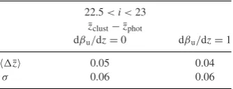
Table 1. Comparison between the mean clustering redshift and the mean photometric redshift from the distributions. This comparison is done when consid-ering dβu/dz=0 and dβu/dz=1. In both cases, the two methods are in agreement.
22.5<i<23 ¯
zclust−z¯phot
dβu/dz=0 dβu/dz=1 ¯
z 0.05 0.04
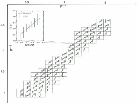
[image:6.595.343.511.658.722.2]Figur
e
7.
Cluster
-z
(black
points)
and
photo-z
d
istrib
utions
in
each
cell
of
the
all
colour
-space
for
iunk
<
22.5.
The
top-left
p
anel
sho
w
s
the
ev
olution
o
f
the
mean
redshift
with
colours.
A
zoom
for
a
gi
v
en
cell
is
sho
w
n
in
the
bottom-right
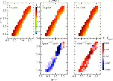
Figure 8. Top panel: mean redshift evolution through colour-space for both reference and unknown samples. Bottom panel: difference between the estimated mean redshift – cluster or photo-z – and the true mean redshift from spectroscopic measurements. One can notice a bad region aroundg−r=1.2 for photo-z. This points out a systematic effect in the photo-z measurements.
Since we are not looking at the spectral energy distribution but at the clustering of objects and since all objects cluster with each other – regardless of their magnitude – we expect a signal (M13; Rahman et al.2016a,b).
Nevertheless, since at a given redshift fainter objects are less massive, we can expect a lower signal than in the previous case. To illustrate this, we use the same reference population used previously withiref<22.5 but we select objects from the unknown sample with
22.5<iunk<23. This leads to an unknown faint sample made of Nu=88 000 galaxies. To be coherent with the previous case, we
build tomographic subsamples ofNu=3000 galaxies.
The resulting clustering-based redshifts distributions for three selected bins that span the all redshift range are shown in black in Fig.6. The measurements of all bins are available online. By computing the quantity ¯zclust−¯zphotfor each distribution, one can
estimate ¯zand theσand then compare cluster-z to photo-z; see Table1.
One can see that clustering-redshift distributions are in agreement with photo-z PDFs. Indeed, we find ¯z =0.05 and 0.04 andσ= 0.06 when considering dβu/dz=0 and dβu/dz=1, respectively.
This demonstrates that the signal could be detected even when the reference and unknown populations do not have the same magnitude limit.
In the context of large imaging experiments, the requirements on spectroscopic redshifts are challenging. In particular, it is difficult to make complete spectroscopic samples down to magnitudesiAB=24
which is the magnitude limit of large imaging surveys likeEuclid. This property of clustering redshift is therefore of great interest.
5 C O L O U R S A M P L I N G
In this section, we aim at freeing the clustering-based redshift es-timation technique from the need of photometric redshifts to
pre-select subsamples localized in redshift and quantify the resulting accuracy.
5.1 Magnitude limit for both samples:i<22.5
First, we look at an unknown population with the same limiting mag-nitude of the reference sample. In this case, we expect the reference sample to be a representative sample of our unknown population. Then, the colour–redshift relation of both samples should be the same on average.
To reduce the effect of the clustering amplitude evolution with redshift of the unknown sample,βu(z), we build subsamples in
colour-space. Working on the (g−i;g−r) plane, we choose a bin-ning size of g−r/i=0.1. By construction, the redshift distribution
in each of these cells will be narrower than the one of the initial sample.
Then we measure the clustering redshift distribution in each cell. All these distributions across the colour-space as well as their corre-sponding photometric and spectroscopic redshift distributions can be seen in Fig.7. The central part of this plot shows the redshift distribution evolution with colours.
Table 2. Comparison between the mean spectro/ photo/cluster-z when considering dβu/dz=0. The bias and scatter of these two approaches are similar when comparing to spectroscopic redshift.
i<22.5 ¯
zphot−¯zspec ¯zclust−z¯spec
– dβu/dz=0
¯
z 0.02 0.02
σ 0.04 0.03
¯
zcl−z¯spec and ¯zph−z¯spec. One can notice the large residuals for
photo-z at (g−i,g−r)∼(2.2, 1.2). They reveal the presence of a systematic effect affecting the photo-z estimate. One can note that the template library has been calibrated with the CFHTLenS optical photometry whose absolute calibration differs by∼0.15 mag in the zband in comparison with the T0007 one (Moutard et al.2016b). This could explain part of the photo-z bias that is observed for red galaxies. We leave to a future work a more detailed exploration of this effect.
To compare, in a more quantitative way, the ability of cluster-z to reproduce the colour–redshift relation compared to photo-cluster-z, we compte the residual ¯zcl/ph−z¯specand summarize the results in
Table2. We find ¯z =0.02 for cluster-z and photo-z while they haveσ=0.02 and 0.03, respectively. This shows that in the colour sampling approach, cluster-z and photo-z have similar accuracy with respect to spectro-z. Nevertheless, one can note that here we use only
three bands to extract subsamples from the unknown population of objects. The resulting cluster-z are compared to photo-z while photo-z were obtained by combining optical and near-infrared data. This is encouraging because there is still plenty of information to be added. Other galaxy properties such as size, brightness and ellipticity can be used in addition to the colours to improve the cluster-z estimation.
5.2 Evolution of the unknown clustering amplitudeβu(z)
In this section, we investigate the validity of the assumption made on the evolution of the clustering amplitude of the unknown sample,
βu(z).
Since we know the photometric redshifts for the unknown popu-lation, we can use them to estimate the true evolution with redshift of the clustering amplitude,βu(z). To do so, we apply the same
procedure used in the measurement of the reference sample clus-tering amplitude,βr(z)(see Section 3.1.3) following equation (8).
This procedure is applied in each cell of the colour-space. Results are shown in Fig.9where we report the measuredβu(z) based on
photometric redshifts (in black), whereas in Fig.2and in the equa-tions of Section 2,βis a function ofzspec∼ztrue. One can note that
in these regions of the colour-space, the clustering amplitudeβu(z)
seems to evolve linearly with redshift. For this reason, we also show a linear fit (in green).
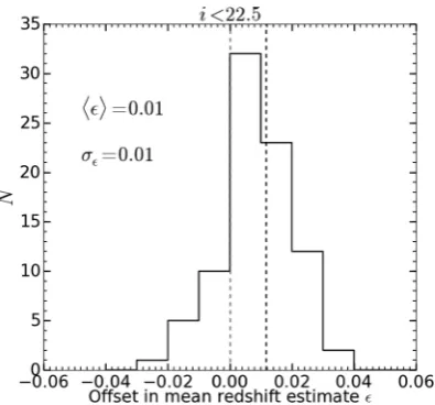
Based on these measurements, we can then compute the offset in the mean redshift, ≡z¯estimated−z¯true, due to the non-evolution
hypothesis we made on the unknown clustering amplitude:
[image:9.595.73.523.367.703.2]Figure 10. Offset in the mean redshift estimates due to the evolution of the unknown clustering amplitudeβu(z). Considering no evolution forβu leads to a bias of 0.02 in the mean redshift recovered by the clustering-based redshift estimation method.
Table 3. Same table than Table2but we add in grey the re-sult when considering dβu/dz=1. This slightly improves the clustering redshift measurements.
i<22.5 ¯
zphot−z¯spec z¯clust−¯zspec
– dβu/dz=0 dβu/dz=1 ¯
z 0.02 0.02 0.01
σ 0.04 0.03 0.02
dβu/dz= 0. The histogram showing the resulting offsets in the
mean redshift estimates is visible in Fig.10. In this case, the effect of considering dβu/dz=0 is a bias of the order of 0.02 in the mean
redshift estimate.
Moreover, since the clustering amplitudes we measured seem to be linear in redshift, we can estimate the cluster-z distributions obtained in Section 5.1 when considering dβu/dz=1 in equation (9)
instead of dβu/dz=0. The results of these new measurements are
summarized in Table3.
Finally, we combined all cluster-z measurements to derive the global redshift distribution in Fig. 11. The top panel shows the two photo-z distributions as well as the global clustering redshift distributions when accounting or not for a linear evolution ofβu(z).
These distributions are obtained by summing the distributions from each cells in colour-space including cells located in the bad region of the photo-z map(see Fig.8). Considering a linear evolution for βu(z) allows us to correct the small distortion of the distribution.
As expected, it appears that the no-evolution assumption tends to slightly underestimate the number of galaxies at low redshift and to slightly overestimate it at high redshift.
The bottom panel of Fig.11shows the same quantities but when summing the distributions only from the ‘good’ cells in colour-space. In this case, we excluded cells located in the bad region of the photo-z map, i.e. cell in the two columns atg−r∼1.2.
5.3 Fainter unknown sample: 22.5<i<23
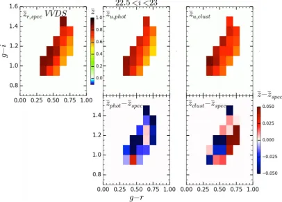
[image:10.595.65.263.55.239.2]In this section, we apply the same sampling approach in colour-space as previously but we use the fainter unknown sample defined in Section 4.3 with 22.5<iunk<23.
Figure 11. Top panel: global redshift distribution estimated by photo-z (green and dashed green), spectro-z (blue) and by cluster-z (black dots) for dβu/dz=0. Red dots correspond to cluster-z with dβu/dz=1. These distributions are obtained by adding the distributions of the all cells of the colour-space, including the bad region visible in Fig.8. Bottom panel: as the top panel but excluding cells in the two columns aroundg−r∼1.2.
This time the colour–redshift relation of both samples are not sup-posed to be the same. To check our results, we then used VVDS data (Le F`evre et al.2005,2013) for which we corrected the magnitudes to be calibrated in the same way than the CFHTLS data.
The VVDS data are then selected to have 22.5<i<23 leading to a complete sample of∼1000 sources. Since this sample is very small and cover an area smaller than VIPERS, one can only expect to have agreement on averaged statistical properties due to cosmic variance.
Then we computed the corresponding clustering redshift distri-butions visible in Fig.12. Those distributions were computed by considering dβu/dz=1.
Fig.13shows the resulting colour–redshift map in the top panels. The corresponding residuals for the faint colour sampling analysis are in the bottom panels. Due to the low number of spectroscopic sources, the residuals are all within the stochastic noise of the mean redshift estimate which can be estimated to be∼0.1. The summary statistics of these measurements are shown in Table4.
In the top panel, we found ¯z =0.03 andσ=0.05 for photo-z and ¯z =0.05 andσ =0.07 for cluster-z when considering no evolution with redshift forβu, while we found ¯z =0.04 and
σ=0.06 when considering dβu/dz=1, in the bottom panel. In both
cases, the cluster-z and photo-z measurements are in agreement. Finally, we combine all distributions from Fig.12and reconstruct the global clustering redshift distribution of the fainter unknown population (see Fig.14). As we could expect, we found results in good agreement between photo-z and cluster-z.
[image:10.595.62.265.330.401.2]Figur
e
12.
Cluster
-z
(black
points)
and
photo-z
d
istrib
utions
in
each
cell
of
the
all
colour
-space
for
22.5
<
iunk
<
23.
The
top-left
p
anel
sho
w
s
the
ev
olution
o
f
the
mean
redshift
with
colours.
A
zoom
for
a
gi
v
en
cell
is
sho
w
n
in
the
bottom-right
Figure 13. Top: mean redshift evolution through colour-space for the unknown sample and for spectroscopic data from VVDS. Bot: difference between the estimated mean redshift – cluster or photo-z – and the true mean redshift from VVDS spectroscopic measurement. The residuals are all within the stochastic noise of the mean redshift estimate.
Table 4. Same table than Table3but we add in grey the results when considering dβu/dz=0 and dβu/dz=1 in the case where the unknown population is fainter than the reference sample.
i<22.5 22.5<i<23
¯
zphot−z¯spec z¯clust−z¯spec z¯phot−z¯spec z¯clust−z¯spec
– dβu/dz=0 dβu/dz=1 – dβu/dz=0 dβu/dz=1
¯
z 0.02 0.02 0.01 0.03 0.05 0.04
σ 0.04 0.03 0.02 0.05 0.07 0.06
Figure 14. Comparison between the global redshift distributions of the unknown sample measured by cluster-z with dβu/dz=1 (red points), photo-z (green line), spectro-photo-z from VVDS (blue line).
fainter than the population of reference. As said previously, it is difficult to make faint complete spectroscopic samples. This prop-erty of clustering redshifts could be of great interest. Moreover, we remind the reader that we use only three bands to subsample the unknown population, whereas photo-z were obtained by combining optical and near-infrared data. We also remind that the spectroscopic distribution visible in blue is not the exact solution since it is a very small sample. Only averaged quantities should be compared.
6 S U M M A RY
We have explored and quantified the ability of clustering-based redshift using VIPERS and CFHTLS. The method adopted in this paper follows the one presented inM13.
(i) We demonstrated our ability to measure the clustering red-shift distribution using a tomographic photo-z sampling. We found similar accuracy between photo-z and cluster-z.
accuracy is similar to photometric redshift. This suggest that the reference sample do not need to be representative of the unknown sample. This property could be of great interest to estimate redshifts in the context of future large surveys.
(iii) We have removed cluster-z from requirement of photo-z by selecting subsamples in colour-space. This allows the cluster-z measurement to be independent of the photometric redshift. That means that cluster-z does not suffer from possible systematics due to the photo-z procedure. Both methods could then be used to validate the other one. One could also try to combined them together.
(iv) We used the last two points to explore the ability of the clustering-based redshift estimation method to probe the redshift distribution of a sample in a magnitude range fainter than and non-overlapping with the reference population, independently of photometric redshift. As said previously, such property could be of great interest in the context of future large imaging surveys, like the
Euclid space mission.
It is important to notice that in some case, e.g. for a galaxy population with strong scale-dependent bias, the local approach could not be sufficient. This would lead to a biased estimate of the redshift distribution. Since the galaxy bias is a strictly increasing function with redshift (Fry1996; Tegmark & Peebles1998), this would induce an under/overestimation of the cluster-z distribution at low/high redshift. Also cosmic variance can affect these results in particular in Section 5.3 when comparing cluster-z to VVDS spectroscopic data.
In future works, we will study in more detail within simulations the accuracy reachable using this method in the context ofEuclid. We will also investigate the number of reference objects and num-ber of filters needed to reach theEuclidphoto-z requirements, alone and/or when combined with photo-z. Also, the clustering properties of galaxies beyondz=1 could affect the measurement. This will be explored in future works. It is important to realize that the per-formance of this approach will keep increasing, mostly because of the increase of the spectroscopic data. Indeed, for a given unknown population, the statistical noise will decrease with each new spectro-scopic redshift, and also because there is still plenty of information to be added to break the colour-redshift degeneracy. For example, one can add other kind of information such as size, brightness, ellipticity. These points will also be explored in a future work.
AC K N OW L E D G E M E N T S
VS is particularly grateful to Brice M´enard, without whom this paper would not have been possible. His advices and many use-ful discussions have been essential for the development of this project. VS also thanks Mubdi Rahman for useful discussions. VS acknowledges funding from the French ministry for research, Universit´e Pierre et Marie-Curie (UPMC) and the Centre National d’Etudes Spatiales (CNES) through the Convention CNES/CNRS N◦140988/00 on the scientific development of VIS and NISP in-struments and the management of the scientific consortium of the Euclid mission. VS acknowledges the Euclid Consortium and the Euclid Science Working Groups.
This work is also based on observations collected at the Euro-pean Southern Observatory, Cerro Paranal, Chile, using the VLT under programs 182.A-0886 and partly 070.A-9007. This paper is also based on observations obtained with MegaPrime/MegaCam, a joint project of CFHT and CEA/DAPNIA, at the CFHT, which is operated by the National Research Council (NRC) of Canada, the Institut National des Sciences de l’Univers of the Centre National de
la Recherche Scientifique (CNRS) of France, and the University of Hawaii. This work is based in part on data products produced at Ter-apix available at the Canadian Astronomy Data Centre as part of the CHFTLS, a collaborative project of NRC and CNRS. The VIPERS web site ishttp://www.vipers.inaf.it/. This research makes use of the VIPERS-MLS data base, operated at CeSAM/LAM, Marseille, France. VIPERS-MLS is supported by the ANR Spin(e) project (ANR-13-BS05-0005,http://cosmicorigin.org). This work is based in part on observations obtained with WIRCam, a joint project of CFHT, Taiwan, Korea, Canada and France. The TERAPIX team has performed the reduction of all the WIRCAM images and the preparation of the catalogues matched with the T0007 CFHTLS data release. This work is based in part on observations made with
theGalaxy Evolution Explorer(GALEX).GALEXis a NASA Small
Explorer, whose mission was developed in cooperation with the CNES of France and the Korean Ministry of Science and Tech-nology. GALEX is operated for NASA by the California Institute of Technology under NASA contract NAS5-98034. This research uses data from the VIMOS VLT Deep Survey, obtained from the VVDS data base operated by Cesam, Laboratoire d’Astrophysique de Marseille, France.
We also acknowledge the crucial contribution of the ESO staff for the management of service observations. In particu-lar, we are deeply grateful to M. Hilker for his constant help and support of this program. Italian participation to VIPERS has been funded by INAF through PRIN 2008 and 2010 pro-grams. LG and BRG acknowledge support of the European Re-search Council through the Darklight ERC Advanced ReRe-search Grant (# 291521). OLF acknowledges support of the European Research Council through the EARLY ERC Advanced Research Grant (# 268107). AP, KM, and JK have been supported by the National Science Centre (grants UMO-2012/07/B/ST9/04425 and UMO-2013/09/D/ST9/04030), the Polish–Swiss Astro Project (co-financed by a grant from Switzerland, through the Swiss Contribu-tion to the enlarged European Union). WJP and RT acknowledge financial support from the European Research Council under the Eu-ropean Community’s Seventh Framework Programme (FP7/2007-2013)/ERC grant agreement n. 202686. WJP is also grateful for support from the UK Science and Technology Facilities Council through the grant ST/I001204/1. EB, FM and LM acknowledge the support from grants ASI-INAF I/023/12/0 and PRIN MIUR 2010-2011. LM also acknowledges financial support from PRIN INAF 2012. YM acknowledges support from CNRS/INSU (Institut National des Sciences de l’Univers) and the Programme National Galaxies et Cosmologie (PNCG). CM is grateful for support from specific project funding of theInstitut Universitaire de Franceand the LABEX OCEVU. Research conducted within the scope of the HECOLS International Associated Laboratory, supported in part by the Polish NCN grant DEC-2013/08/M/ST9/00664.
R E F E R E N C E S
Albrecht A. et al., 2006, preprint (arXiv:astro-ph/0609591) Amendola L. et al., 2013, Liv. Rev. Relativ., 16, 6 Bernstein G., Huterer D., 2010, MNRAS, 401, 1399 Coleman G. D. et al., 1980, ApJS, 43, 393 Connolly A. J. et al., 1995, AJ, 110, 2655 Cooper M. C. et al., 2006, MNRAS, 370, 198 Davis M., Peebles P. J. E., 1983, ApJ, 267, 465 Fry J. N., 1996, ApJ, 461, L65
Huterer D. et al., 2006, MNRAS, 366, 101 Knox L., Song Y.-S., Zhan H., 2006, ApJ, 652, 857 Landy S. D., Szalay A. S., Koo D. C., 1996, ApJ, 460, 94 Laureijs R. et al., 2011, preprint (arXiv:1110.3193) Le F`evre O. et al., 2005, A&A, 439, 845
Le F`evre O. et al., 2013, A&A, 559, A14 McQuinn M., White M., 2013, MNRAS, 433, 2857 Ma Z., Hu W., Huterer D., 2006, ApJ, 636, 21 Marulli F. et al., 2013, A&A, 557, A17
Matthews D. J., Newman J. A., 2010, ApJ, 721, 456 Matthews D. J., Newman J. A., 2012, ApJ, 745, 180
M´enard B., Scranton R., Schmidt S., Morrison C., Jeong D., Budavari T., Rahman M., 2013, preprint (arXiv:1303.4722) (M13)
Moutard T. et al., 2016a, A&A, 590, A102 Moutard T. et al., 2016b, A&A, 590, A103 Newman J. A., 2008, ApJ, 684, 88 Newman J. et al., 2015, ApJ, 63, 81
Phillipps S., Shanks T., 1987, MNRAS, 229, 621
Rahman M., M´enard B., Scranton R., Schmidt S. J., Morrison C. B., 2015, MNRAS, 447, 3500 (R15)
Rahman M., M´enard B., Scranton R., 2016a, MNRAS, 457, 3912 Rahman M., Mendez A. J., M´enard B., Scranton R., Schmidt S. J., Morrison
C. B., Budav`ari T., 2016b, MNRAS, 460, 163 Schmidt S. J. et al., 2013, MNRAS, 431, 3307 Schmidt S. J. et al., 2015, MNRAS, 446, 2696
Seldner M., Peebles P. J. E., 1979, ApJ, 227, 30 Sun L. et al., 2009, ApJ, 699, 958
Tegmark M., Peebles P. J. E., 1998, ApJ, 500, L79 Thomas S. A. et al., 2011, MNRAS, 412, 1669 Zhan H., 2006, J. Cosmol. Astropart. Phys., 8, 8 Zhan H., Knox L., 2006, ApJ, 644, 663
S U P P O RT I N G I N F O R M AT I O N
Additional Supporting Information may be found in the online ver-sion of this article:
Scoltez_Clustering_redshift_Paper.tar supplementary_online_material.tar
(http://www.mnras.oxfordjournals.org/lookup/suppl/doi:10.1093/ mnras/stw1500/-/DC1).
Please note: Oxford University Press is not responsible for the content or functionality of any supporting materials supplied by the authors. Any queries (other than missing material) should be directed to the corresponding author for the article.