Computer aided parameter selection for resistance exercise using machine vision based capability profile estimation

O R I G I N A L P A P E R

Computer-Aided Parameter Selection for Resistance Exercise

Using Machine Vision-Based Capability Profile Estimation

Ognjen Arandjelovic´1

Received: 12 April 2017 / Accepted: 14 July 2017

The Author(s) 2017. This article is an open access publication

Abstract The penetration of mathematical modelling in sports science to date has been highly limited. In particular and in contrast to most other scientific disciplines, sports science research has been characterized by comparatively little effort investment in the development of phe-nomenological models. Practical applications of such models aimed at assisting trainees or sports professionals more generally remain nonexistent. The present paper aims at addressing this gap. We adopt a recently proposed mathematical model of neuromuscular engagement and adaptation, and develop around it an algorithmic frame-work which allows it to be employed in actual training program design and monitoring by resistance training practitioners (coaches or athletes). We first show how training performance characteristics can be extracted from video sequences, effortlessly and with minimal human input, using computer vision. The extracted characteristics are then used to fit the adopted model i.e. to estimate the values of its free parameters, from differential equations of motion in what is usually termed the inverse dynamics problem. A computer simulation of training bouts using the estimated (and hence athlete specific) model is used to predict the effected adaptation and with it the expected changes in future performance capabilities. Lastly we describe a proof-of-concept software tool we developed which allows the practitioner to manipulate training parameters and immediately see their effect on predicted adaptation (again, on an athlete specific basis). Thus, this work presents a holistic view of the monitoring–

assessment–adjustment loop which lies at the centre of successful coaching. By bridging the gap between theo-retical and applied aspects of sports science, the present contribution highlights the potential of mathematical and computational modelling in this field and serves to encourage further research focus in this direction.

Keywords Capability profileStrengthForce

EstimationComputer visionSoftwareWeight training

Introduction

Sports science is a discipline characterized by a strong focus on practical application. Ultimately, the aim of any research in this field is to facilitate advancement in some aspect of the athletic endeavour. The nature of such advancement may take on many forms. An improvement in performance may be achieved through the use of a novel training modal-ity [1–3] or better training parameter selection [4, 5], for example. Alternatively, strategies to enhance intra-train-ing [6] or inter-training [7,8] recovery rates may be devised. Injury prevention methods [9] or methods for accelerating rehabilitation [10], over time albeit indirectly can also be seen to contribute to improved performance. While certainly not an exhaustive list, the aforementioned elements of an integral training regime have been attracting the most attention from researchers and practitioners. The complexity emerging from the interrelatedness of these elements illus-trates the breadth of potential avenues for further study and potential scientific contribution to the sports community.

In broad terms, the development of a novel idea in sport science comprises three distinct challenges before reaching the stage of general acceptance by the practitioners. The first of these concerns the pursuit of data collection by & Ognjen Arandjelovic´

[email protected]; [email protected]

1 _{School of Computer Science, Universtiy of St Andrews,}

means of empirical study. Indeed, this aspect of research has been dominating sports science for most of its existence, producing a consistently expanding corpus of available data. The accumulation of empirical findings facilitates the second challenge—the understanding of the underlying physiological mechanisms. This is effected by the unifica-tion of regularities in the observed data by means of phe-nomenological models. Such models effectively reduce the total information content needed to describe a particular phenomenon and are subjected to scrutiny through the predictions they produce. In this final stage the model is applied in practice, in the context of athletic training.

This paper focuses on the final of the aforementioned developmental stages. Specifically, it considers several out-standing problems associated with the application of a recently proposed physiological model underlying resistance training performance and adaptation and extends the previous work described in [11]. Herein, we expand on the technical detail of each of the stages of the framework in detail, present additional discussion, and explain how different parameters of the framework can be estimated either directly from data or based on evidence in the existing literature. Moreover, we present additional empirical experiments and findings and discuss the performance of the proposed method in light of these. Finally, we present a more comprehensive description of the proof-of-concept software tool which we developed and which implements the proposed algorithms.

The remainder of the paper is organized as follows. A list of the most commonly used mathematical symbols and their explanations is given in Table1. The estimation

of measurable performance characteristics from realistic, loosely constrained videos of athletes in training is addressed in Sect.2. The process of estimation of free model parameters from said characteristics is the subject of Sect.3and the subsequent use of the model to guide future training choices in a manner tuned to a specific athlete and exercise of Sect.4. A summary and a discussion of promising future work directions are presented in Sect.5.

Image-Based Extraction of Performance

Characteristics

The central concept in the computational model introduced in [12] is the capability profile of an athlete in a given exercise. It is instrumental in predicting performance as well as in capturing the nature and magnitude of training adaptations. An athlete’s capability profile F^ for a given exercise is defined as the maximum force that the athlete can exert against the load in the exercise as a function of the load’s position (commonly elevation)dand velocityv:

^

FF^ðd;vÞ: ð1Þ

ConceptuallyF^ðd;vÞcan be thought of as a generalization of the force–length [13–15] and force–velocity character-istics [16,17] of an isolated skeletal muscle to an arbitrary and in practice usually biomechanically complex exer-cise [12]. Force–length and force–velocity characteristics, while trainable [18] and variable between different people as well as across different muscles of the same person,

Table 1 A summary of the key mathematical notation used in this paper

Symbol Description

Image

Fi ith input video frame as a matrix of pixels

x Horizontal location of a pixel i.e. pixel column index y Vertical location of a pixel i.e. pixel row index

Wi Region of interest in framei

TjðiÞ Vertical location ofjth image feature of interest in framei

d Displacement of a feature in pixels relative to its bottom-most location Physical

t Time from the beginning of the first repetition

d Displacement/elevation of the load from the bottom-most position v Velocity of the load; positive for the concentric effort

F Effective force exerted by the athlete against the load

wn Athlete’s measuredn-repetition maximal load (nRM)

^

wn Estimate of athlete’sn-repetition maximal load

Model

^

F Athlete’s capability profile for a particular exercise TF Athlete and exercise-specific fatigue time constant

generally share the same functional form. However, this is generally not the case for a capability profile corresponding to an arbitrary exercise. The universal characteristics of force production for individual muscles are modulated by the plurality of involved musculature, attachment structure of individual muscles and the change in the biomechanics throughout the lift. It is an important observation that in the model proposed in [12] these are not modelled sepa-rately—all performance prediction and adaptation experi-enced over time is based on the corresponding capability profile which captures the total effective force exerted against the load.

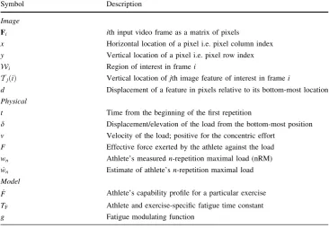
The model is employed by predicting exercise perfor-mance first. This is achieved by formulating a differential equation governing the motion of the load. Using its numerical approximation, a computer simulation is applied to predict the variation in the elevation of the load through time. The effective force which the athlete can exert against the load at different stages of the movement mod-elled as the athlete’s capability profile which is additionally modulated by an exponential decay capturing fatigue accumulation which takes place over time. Simulation results are then used to infer the adaptational stimulus, which manifests itself through a fed-back modification of the capability profile. The key elements of the training– adaptation cycle are illustrated schematically in Fig.1. For further in-depth technical detail on the model, the reader is referred to the original publication [12].

The aim of the work presented in this paper was to develop a framework which facilitates the application of the aforementioned model in training practice. The key

contributions include: (1) a method for the estimation of the free parameters of the model from data which can be readily acquired without the use of specialized equipment, large cost or user effort, and (2) a proof-of-concept soft-ware tool which implements the proposed framework allowing it to be used for planning real-world resistance training regimens.

Overview of the Proposed Framework

The first contribution of this paper and the focus of this section is an algorithm for estimating the motion of the load in resistance exercise. This is a crucial element in the pipeline described in subsequent sections. Specifically, the reconstruction of an athlete’s capability profile [12], which is based on the elevation–velocity characteristics, and the corresponding force exerted against the load in the per-formed lifts, are both inferred from the motion extracted here.

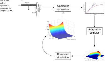
The key stages of the proposed method are illustrated conceptually in the diagram shown in Fig.2. The process beings with the detection of so-calledinterest pointsin the starting frame of the raw input video. Overlaid on the original image these are displayed to the user who selects a region corresponding to the load used for exercise. Then, each interest point within this region of interest is tracked until the completion of the video producing a series of continuous motion tracks, one for each interest point. Information from all extracted tracks is polled together to reliably infer the overall motion of the load which is then processed further to extract the corresponding variation in

velocity and the effective force exerted against the load. The starting and terminal times of individual repetitions (and their concentric and eccentric portions) are extracted here too. Each of the aforementioned steps is described in detail next.

Detection of Reliable Tracking Features

ConsiderF1, the initial frame of an input video sequence

represented as a greyscale image, with the value of the pixel at the image locationx¼ ðx;yÞdenoted asFðx;yÞ(or equivalentlyFðxÞ, depending on convenience). The corre-sponding Gaussian scale-space Sðx;y;sÞ is a three-di-mensional volume defined as follows:

Sðx;y;sÞ ¼F1ðx;yÞ xyGðx;y;srÞ ð2Þ

wherexydenotes convolution overxandy, andGðx;y;srÞis a two-dimensional isotropic Gaussian distribution with the diagonal elements of the covariance matrix equal toðsrÞ2:

Gðx;y;srÞ ¼ 1

2ps2_r2exp

x2_þy2

2s2_r2

: ð3Þ

Heresis the so-called scale parameter and it governs the degree of image blur, suppressing image features of a lesser spatial extent than pffiffis. In practice, the scale-space is quantized to only a discrete set of values of s¼s1;. . .sm usually chosen as logarithmically equidistant with a spacing which gives an integer number of scale levels in an octave:

9q2N;8i1:log₂ðsiþ1=siÞ ¼q: ð4Þ

Characteristic image interest points can be readily localized from Sðx;y;sÞas the loci of at which appearance change with scale (at some scale-space level) exhibits maximum rate of change. To ensure repeatability, as proposed by Lowe [19], this initial list is further narrowed down by accepting only those loci which are well localized by requiring both eigenvalues of the corresponding Hessian to be sufficiently large [20]. This process ensures that low contrast loci or line like regions are rejected. An example of a typical result is shown in Fig.3a.

Feature Seeding

By construction, interest points are image loci with locally characteristic appearance. As such, they are promising candidates for reliable tracking of motion through time. However, our specific aim here is to extract the motion of the load lifted by the athlete—the video sequence may contain other, confounding sources of motion which are not of interest. For example, there may be other trainees moving in the background. Thus, we seek to restrict our attention to those interest points which are within the region corresponding to the moving load.

image corresponding to the load used by the athlete. The loci of detected interest points, which are marked on the displayed image, thus serve to guide the user who can choose a region with their maximal number. A typical example is illustrated in Fig.3a with a magnification of the user-selected region of interest shown in Fig.3b and the associated image patches in Fig.4.

Feature Tracking

Having located a set of discriminative image loci of interest, the goal is to track them over time. The method-ology employed here is similar to that first proposed by Lucas and Kanade [21] and subsequently further developed by Tomasi and Kanade [22], and Shi and Tomasi [23]. There are two key differences in the approach taken here: in the initialization of the tracked windows and in the search for the optimal frame-to-frame wrapping parameters (see [24, 25]). Unlike Shi and Tomasi whose choice of tracking windows is based on the spatio-temporal gradient

matrix corresponding to the first two video frames, here the tracked regions surrounding interest points are detected as described in Sect.2.2. The dimensions of each square region are set equal to the detection scale of the corre-sponding interest point.

As in the previous work, tracking is formulated as an optimization problem, whereby the region of interestWin frame Fi is localized in the subsequent frame Fiþ1 by

estimating the set of parameters a2R6 _{of an affine}

transformation which maps Wonto a region inFiþ1, such

that the observed image difference is minimized. A mod-ification introduced here is to estimateausing a three-level pyramidal coarse-to-fine scheme whereby the initial esti-mate is made using quarter-resolution images, which is then refined at half-resolution and finally full resolution. This serves both to increase the speed of convergence as well as the robustness of the estimate by preventing the iterative gradient descent (described next) from getting stuck to a locally optimal value. Formally, at each level of the pyramid, we wish to minimize:

(a)

(b)

Fig. 3 aThe original frame with detected features overlaid asyellow dotsandba close-up surrounding the interest region outlined by the user (purple line)

eðaÞ ¼X

x2W

Fiþ1ðxaÞ FiðxÞ

2

; _ð5Þ

wherex¼ ½xyT is a vector corresponding to image loca-tion (x,y), and:

xa ¼

ð1þa1Þxþa3yþa5

a2xþ ð1þa4Þyþa6

: ð6Þ

Minimization of the error term eðaÞ is a nonlinear optimization task which can be solved through an iterative steepest descent scheme. Using the first order Taylor series expansion of the expression in Eq.5,eðaÞcan be approx-imated by^eðaÞ:

eðaÞ ^eðaÞ ¼X

x2W

Fiþ1ðxaÞ þ rFiþ1

oxa

oa DaFiðxÞ

2

ð7Þ

This is a quadratic minimization problem, which can be solved in a closed form. A simple but cluttered analysis shows that minimal^eðaÞis achieved for:

Da¼ X x

oxa oa

T

rFiþ1TrFiþ1

oxa oa

( )1

X

x

rFiþ1

oxa oa

T

FiðxÞ Fiþ1ðxaÞ

ð8Þ

Equation8 and the update of the warping parameter aðjþ_i 1Þ¼aðjÞ_i þDaðjÞ_i are applied until convergence i.e. until the magnitude of the update fails to exceed a tolerance threshold on the parameter errorkDaðjÞ_i k [26].

Robust Motion Estimation

The tracking algorithm described in the previous section follows the movement of a particular local feature within the region of interest, initially corresponding to an auto-matically detected interest point. However, generally, the region of interest contains many features, each of which produces a track:

Tn¼xnð0Þ;. . .;xnðknDtÞ fornth feature ð9Þ

As indicated by different maximal time step indiceski, the tracks may be of different durations—a feature once lost in tracking is not re-spawned.

An example of a set of tracks extracted from a typical lifting video sequence is shown in Fig.5a. Each thin (and blue, if viewing in colour) line is the vertical track of a single feature. Note different starting values of elevation of different features’ tracks—these correspond to different initial locations and are not of relevance here. It is the coherence in their relative motion which is being exploited

in computing the mean load displacement, shown as the superimposed thick red line.

As will become apparent in Sect.3, precise tracking of the load is crucial for the accurate estimation of the vari-ation in the force exerted by the trainee. Here we use the entire set of obtained feature tracks to more robustly infer their shared translatory motion, that is, the motion of the rigid load they correspond to. Let, without loss of gener-ality, k1 k2 kn. We compute the location of the load at time kDt as follows. If Dk is the set of displace-ments at kDt at mostDpixels smaller or greater than the median displacement atkDt:

Vk¼fxiðkDtÞ xið0Þ:ki kg ð10Þ

Dk¼ d:d2V^ kdl1=2ðVÞk D

n o

ð11Þ

Then the displacement of the bar atkDtis computed as the robust mean:

dðkDtÞ ¼ 1 jDkj

X

d2Dk

d _ð12Þ

The result of applying this approach is illustrated in Figs. 5and6.

Estimating Physical from Observed Image Motion

(a)

(b)

(c)

(d)

Fig. 5 aTracks of vertical displacement over time of features of interest (thin blue lines) and the robust overall motion estimated using the proposed algorithm (thick red line). bOverall vertical displace-ment track, marked with semantic labelling corresponding to different

stages of a set of repetitions.c The detected starting and terminal points of the concentric portions of each completed repetition (red circles and dotted vertical lines). d Variation in the vertical displacement of the load during three extracted concentric bouts

dðtÞ ¼KxxðtÞ ð13Þ

The value of the multiplicative constant Kx is deter-mined through simple calibration using a known reference object (e.g. the length of a standard Olympic barbell).

Repetition Segmentation and Concentric Motion Extraction

Generally, the overall motion of the load, extracted in the previous section, captures different aspects of a lifting bout. This is illustrated in Fig.5b. Initially, the athlete is preparing for the lift and the load may exhibit motion as the athlete assumes a comfortable starting pose. This is then followed by alternating eccentric and concentric lifting efforts (not necessarily in that order) separated by usually brief pauses, that is, isometric holds. They facilitate the dissipation of some of the accumulated fatigue, allow the athlete to focus on the forthcoming repetition, catch breath, check body positioning etc. Static holds may follow either the eccentric or the concentric portion of the lift, depending on the biomechanics of a particular exercise. In the bench press or the squat, for example, a natural tendency is to pause after the concentric portion of a repetition. During the execution of the barbell row, the opposite is true, and the pause is more likely after the eccentric effort.

From Performance Characteristics

to the Capability Profile

In the previous section we saw how the variation in the elevation of the load used for resistance exercise can be robustly extracted from video without strong assumptions on the exercise, viewpoint or the appearance of the load. Here our goal is to use these measured performance char-acteristics to infer the athlete’s exercise-specific fitness, that is, in the context of the performance model adopted in this paper, the athlete’scapability profile.

This concept is central to the model employed in the present work and is adopted from [12]. The capability profile is instrumental in predicting performance as well as in capturing the nature and magnitude of training adapta-tions. An athlete’s capability profile for a given exercise was defined as the maximum force that the athlete can exert against the load in that exercise, as a function of the load’s elevation and velocity. Conceptually it can be thought of as a generalization of force–length [27,28] and force–velocity [16, 17] characteristics of an isolated skeletal muscle. Force–length and force–velocity charac-teristics, while trainable and variable between different people as well as across different muscles of the same person, have universal functional behaviour. In contrast,

the capability profile is dependent both on the specifics of a particular exercise as well as athlete’s muscle attachment structure, limb lengths, weight distribution etc [29,30]. As such, it must be estimated directly from performance characteristics, such as those whose extraction was addressed in Sect. 2.

Estimating Velocity and Force Variation

The athlete’s capability profileF^in an exercise is defined as a bivariate function capturing the dependence of the maximum force that the athlete can exert against the load and the load’s elevationd and velocityv. That is:

^

FF^ðd;vÞ: ð14Þ

It is this variation that we wish to infer from a set of motion tracks, each corresponding to a concentric portion of a repetition in a given lift, extracted using the algorithm detailed in Sect.2.

Consider the vector comprising the displacement (eleva-tion) and velocity of the load over time,dðtÞ hdðtÞdð_ tÞiT where a dot over a symbol signifies time differentiation (thus

_ d¼dd

dt is the rate of change of elevation, or velocity, and €

d¼d2_d

dt2is the rate of change of velocity, or acceleration). This

state vector of the load changes throughout the lift, thus making a path P through the two-dimensional elevation– velocity (or capability) plane. The idea proposed here is that the capability profileF^ðd;vÞcan be inferred in the localities of all available pathsPifrom the estimates of the effective force variationFiðtÞalong the said paths.

Velocity, Acceleration and Effective Force

The quantity directly measured from an input video is the elevation of the load. From the position of the load, its vertical velocity must be estimated to obtain capability plane tracksPi, as well as its acceleration from whichFiðtÞ can be computed.

In principle this can be achieved by means of simple numerical differentiation of the elevationdðtÞ. If the vari-ationdðtÞis sampled at equidistant intervalsttk¼kDt, the corresponding instantaneous velocity can be estimated using the well-known three point finite difference approximation:

vk¼ 1

2Dt ðdkþ1dk1Þ: k[0

0: k¼0ðinitial conditionÞ

8 < :

ð15Þ

ak¼ 1

2Dt ðvkþ1vk1Þ: k[0

1

Dt ðvkþ1vkÞ: k¼0

8 > < >

: ð16Þ

where the subscriptkis used to denote the value of a par-ticular variable at timet¼kDt. However, this approach has the undesirable effect of amplifying high frequency noise present in the initial estimates ofdk [31]. The corruption of the desired signal is particularly pronounced with repeated differentiation. On the other hand, the usual practice of simple data smoothing (i.e. smoothing that does not include in its underlying model any constraints that emerge from the semantics of the specific signal—in this case the underlying physics and physiology) prior to differentiation is problem-atic because it can result in physiologically unrealistic force estimates [32]. Instead, to ensure that our known domain specific physical constraints are satisfied, we fit a constrained smoothing cubic spline [33] to load elevation valuesdðkDtÞ and then differentiate the spline itself. Specifically, we construct a spline which minimizes the objective function which comprises two terms: (1) the discrepancy between the observed data (load elevation) and that predicted by the spline, and (2) the spline roughness. Formally, the objective functiondis:

d¼x

X

k

dðkDtÞ dð^kDtÞ

2 |fflfflfflfflfflfflfflfflfflfflfflfflfflfflfflfflfflffl{zfflfflfflfflfflfflfflfflfflfflfflfflfflfflfflfflfflffl} Fitting disagreement

þð1xÞ

Z

t € dðtÞ2dt

|fflfflfflfflfflffl{zfflfflfflfflfflffl} Roughness

;

ð17Þ

where 0 x 1, and the initial condition constraint: dd

dt

t¼0¼v0¼0:

ð18Þ

The value of the weighting parameterxis set empiri-cally and is dependent on the quality of input video (in particular, its resolution and the level of noise associated with the CCD sensor).

Estimation of Effective Force Exerted by the Athlete

The final step in the process of extracting lift characteristics from video proposed in this paper is the estimation of effective force exerted by the athlete and against the load. Having estimated the variation of the load’s position, velocity and acceleration through time, force can be com-puted from the differential equations of motion, that is, by the method of so-called ‘‘inverse dynamics’’. In its most general form, the motion of the load can be described through an equation capturing the dependency of its position don (1) the forceFapplied against the load, (2) the velocity, acceleration and possibly higher order derivatives of the

load’s position, and (3) a set of exercise parametersKwhich include a variety of biomechanical variables. Formally:

0¼wðF;d;d;_ d;€ . . .;KÞ ð19Þ

The application of inverse dynamics then comprises the computation ofFfrom the known values of the remaining quantities in Eq.19. For clarity, we shall consider a few relevant examples next.

Inverse dynamics example 1: free load only The simplest setup of practical relevance involves a free load of massm

lifted by the athlete against gravity. If the variation of the acceleration of the load through time is known, the effec-tive force exerted by the athlete at any timetduring the lift can be computed as:

FðtÞ ¼mhdð€tÞ þgi ð20Þ

wheregis the acceleration due to gravity.

Inverse dynamics example 2: free load with added elastic resistance A more complex system can be obtained by the addition of an elastic resistance component to the free weight, as frequently done by powerlifters using elastic bands [34]. The equation of motion then becomes:

mdð€tÞ ¼FðtÞ mgFEðdÞ; ð21Þ

whereFEðdÞ captures the dependency of the elastic force exerted on the load. This dependency is usually linear so the equation of motion can be rewritten as:

mdð€tÞ ¼FðtÞ mg½kdðtÞ þFE0; ð22Þ

whereFE0 is the elastic force at the bottom-most position

of the load,dðtÞ ¼0. Thus, the force exerted by the athlete at any time t can be computed from the estimates of the load’s position and acceleration as:

FðtÞ ¼mdð€tÞ þgþkdðtÞ þFE0

: ð23Þ

Estimation of effective force: concluding remarks While simple, the two loading scenarios which were provided as examples illustrate the general principle that the effective force exerted by the athlete against the load can be com-puted from the characteristics of the load’s motion (posi-tion, velocity, acceleration etc.) and the physical model of the resistance seen by the load (due to gravity, elastic forces, drag etc.). For a detailed treatment of more complex resistance systems encountered in practice the reader is referred to the relevant previous work [12,35–37].

Fatigue Modelling and Parameter Inference

motion of the load and the prior knowledge of the system dynamics. Under the adopted model, this force is bounded above by the value of the capability profile for the corre-sponding stateF^ðdðtÞ;dð_ tÞÞ, modulated by the accumulated fatigue:

FðtÞ _F^_{ðdðtÞ; dð}_ _{tÞÞ expðt=TFÞ; ð24Þ}

where TF is the person-specific fatigue time constant,

unknown a priori. In simulations reported in [12], and the discussion of a possible approach for model parameter inference, it was assumed that the upper bound in Eq.24 was actually attained at all times. In other words, the ath-lete was assumed to always attempt to maximally accel-erate the load. This assumption was justified by the focus of the original publication on strength and power athletes, such as powerlifters, who indeed do observe this practice in training [38]. However, the aim in the present work is to devise an approach more widely applicable and, as will be shown, the aforementioned assumption of continuous maximum exertion does not hold well for maximal sets at intensities lower than 85% (i.e. for maximum sets of more than6 repetitions).

Variable Fatigue Model

Firstly, to account for non-maximum exertion, Eq.24 is here extended to explicitly account for a variable rate of fatigue accumulation. Formally:

FðtÞ ¼F^ðdðtÞ;dð_ tÞÞ gðtÞ; ð25Þ

where 0 gðtÞ 1 is the newly introduced fatigue modu-lating function, and:

dgðtÞ dt ¼

1

TF

gðtÞqðtÞ ð26Þ

The coefficient qðtÞ, where 0 qðtÞ 1, effectively scales the time fatigue constant from its minimum value of

TF attained during maximum exertion. Put differently,

fatigue (captured through g) is accumulated less quickly (governed by dg=dt) when a trainee exerts a lower force. The rate of maximum voluntary force loss is decreased at the time of submaximum effort (lower voluntary force can be sustained for longer time):

qðtÞ ¼FðtÞ=F^ðdðtÞ;dð_ tÞÞ: ð27Þ

Note that whenqðtÞ 1 i.e. whenF^ðdðtÞ;dð_ tÞÞ FðtÞ, the form of the fatigue function becomes simply

gðtÞ ¼expðt=TFÞ, as in the original model [12].

How-ever, in general, becauseqðtÞis a function of time (inferred from observed data as explained in the next section), Eq.26cannot be solved in closed form.

Force–Fatigue Model for Trained Athletes

In the original work by Arandjelovic´ [12] the assumption was that the athlete exerts the maximum force possible at each point in the lift. This force is readily computed using the athlete’s capability profile corresponding to the lift in question and the model of fatigue accumulation. The assumption of continuous maximal exertion is effectively a simple model of force–fatigue management, characterizing how an athlete employs the underlying capability to pro-duce force to complete the lift. In this work, an alternative model is described which is aimed at a broader range of athletes. Our focus is on athletes who explicitly seek per-formance improvement across a range of intensities, unlike powerlifters who are ultimately concerned only with per-formance at the maximal intensity i.e. 100% of one repe-tition maximum (1RM).

Here we consider trained athletes. This allows us to assume that the use of the underlying force production capability is approximately optimized for the training task. Specifically, we assume that for a given training intensity (i.e. load relative to 1RM), the athlete’s force production is such as to complete a repetition with minimize fatigue accumulationthus allowing the athlete to perform the most work (repetitions) at this intensity.

To formalize the above, letLðkÞðdnþ1;vÞbe the negative

logarithm of the fatigue modulating function g(t) at the repetitionk, the load’s positiondnþ1 and velocity v:

LðkÞðdnþ1;vÞ ¼ loggðtÞ: ð28Þ

Then, to meet the assumption of the minimal accumu-lated fatigue, the force exerted by the athlete at each time stepn has to satisfy the following equality:

LðkÞðdnþ1;vÞ ¼ min

v0_2R s

Lðdn;v0Þ þ Dt TF

qðtÞ

¼ min v0_2R s

Lðdn;v0Þ þ

dnþ1dn

TFðvþv0Þ=2

F_^nðdn;vÞ

Fðdn;vÞ

:

ð29Þ

Here, fatigue corresponding to LðkÞðdnþ1;vÞ is minimized

by considering the minimal fatigue achievable at the pre-vious time step atLðkÞðdn;v0Þand the incremental increase in fatigue accumulated in reaching LðkÞðdnþ1;vÞ from

defined by the locusðdn;d_nÞ, the condition that failure does not take place (i.e. the locus ðdn;0Þ) and the maximal velocity that the load can have given the athlete’s capa-bility (corresponding to the maximal force that the athlete can produce). Finally, the repetition has to end with the load velocityvT such that:

vT¼arg min vT

LðkÞðdmax;vTÞ: ð30Þ

This boundary condition enforces global optimality of the repetition i.e. minimizes the total fatigue accumulated in lifting the load.

Inference of model parameters Observe that the nature of lifting performance optimality described by Eq.29 is not such that incremental fatigue at each time step is mini-mized, that is, the term dnþ1dn

TFðvþv0Þ=2 Fnðdn;vÞ

^

Fðdn;vÞ. Rather than being

local, optimization is global. It is by virtue of this assumption that it is necessary to constrain our attention to trained individuals [39]. Specifically, the reader should note that fatigue minimization described by the introduced model is not achieved through conscious efforts of the athlete. Instead, it is an adaptation of the neuromuscular system induced through repeated training bouts.

In mathematical vernacular, the optimization problem of interest is not ‘‘greedy’’. On the other hand, it does exhibit the property of optimality of nested overlapping

subproblems. This is readily apparent by inspection from Eq. 29—the optimal solution at the load positiondnþ1can

be expressed as a function of a locally computable term and the optimal solution corresponding to the position of the load at the preceding time step, that is, dn. Optimization problems of this type are solvable efficiently [40]. How-ever, note that this is not what we are trying to achieve here. Rather than trying to compute the optimal solution, our goal is to infer the underlying model parameters (the athlete’s capability profile) from (1) the optimal solution and (2) the form of the model. The optimal solution is given by the lifting characteristics or, equivalently, the corresponding repetition paths in the capability plane. The form of the underlying model is that described by Eq. 29. The difficulty of this inference is rooted in the global nature of the optimization, that is, in terms of our mathematical model, the loss of local information through summation.

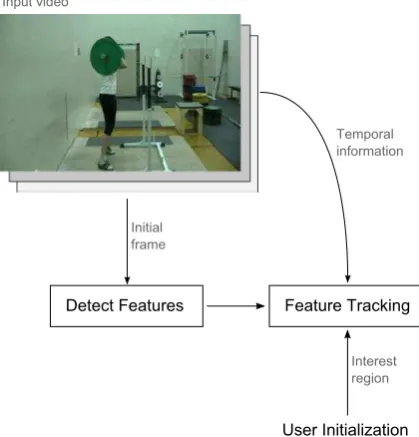
The set-ending repetition Consider the last attempted repetition in a set which ends in momentary muscular failure. Referring back to the illustration in Fig. 7, in the last elementary time interval Dt, the shaded region Rs collapses to a line—the velocity of the load drops to 0 even when maximal possible force is applied by the athlete. This means that the coefficientqðtÞis equal to 1. By means of mathematical induction and working backwards in time, it can be seen thatqðtÞ ¼1 for the entire duration of the final repetition. Thus, we can write:

Fnðdn;vÞ ¼F^ðdn;vÞ exp LðKÞðdn;vÞ

n o

¼_F^_ðdn;vÞ

exp LðKÞð0;0Þ ^t=TF

n o

; ð31Þ

whereKis the index of the final repetition and^ttime since its beginning. It is clear from Eq.31that the values of the capability profile F^ðd;vÞ along the path corresponding to the final repetition can be computed directly up to scale. The global scale of the capability profile is then estimated by matching its prediction with the actual load lifted by the trainee. Lastly, the value of the fatigue time constant TF

was adopted from previous work [12] where it was esti-mated from empirical data to beTF65 s.

Successful repetitions The lifting conditions during the last repetition in a set are rather special—failure to complete the lift results despite athlete’s maximal effort investment. In contrast, the preceding, successful repetitions offer a ‘‘choice’’ (not necessarily conscious, as noted earlier) in the manner force exerted against the load is managed over time, This choice is described mathematically in the form of the optimization in Eq.29. It is the global nature of this opti-mization which makes lifting characteristics measured dur-ing successful repetitions less informative in the reconstruction of the underlying capability profile. Fig. 7 At every point in a successful lift the motion of the load is

constrained. This can be visualized usefully by considering the lift as a path through the capability plane (see Sect.2). In the process of inference of the underlying capability profile, the position of the load at ðdn;d^nÞ constrains its position at the next time increment to a

triangle, defined by the load’s current position ðdn;d^nÞ, the point

which would be reached in the case of subsequent immediate failure

ðdnþ1;0Þand the point which would be reached in the case of athlete’s

Successful repetitions can merely be used to formulate a lower bound on the values of the capability profile along the capability plane paths corresponding to the repetitions. For this reason, in the present work, successful repetitions are not used in the capability profile reconstruction.

Integrating data from multiple sets Repetitions of sets performed by the same athlete but different intensities trace different paths in the capability plane. Thus, performance characteristics at a range of training intensities can be used to infer the functional forms of different regions of the athlete’s capability profile underlying the exercise in consideration.

In practice, sufficient data for accurate reconstruction of the region of the capability profile relevant to the athlete’s performance could be accumulated with ease. This is especially true in the case of cornerstone exercises (e.g. the bench press for powerlifters or the squat for weightlifters) which are practiced with relatively high frequency and volume. Monitoring training performance over only a few sessions would typically suffice. In this paper, to overcome the limited amount of data we had available and extend the area of the capability plane over which capability is esti-mated, we also employ interpolative and extrapolative methods. These are employed while ensuring the confor-mance of the results with constraints derived to the fun-damental physiological principles underlying the capability profile. Specifically, we require that the capability profile is monotonically decreasing in the ‘‘velocity direction’’ i.e. that for any given point in an exercise, maximum effective force that the athlete can exert against the load decreases with the increase in the load’s velocity:

8d;v1\v2:Fðd;v1Þ[Fðd;v2Þ ð32Þ

For a single muscle, Eq.32 follows trivially from Hill’s equation [16]. For an arbitrary number of contributing mus-cles in a complex, compound exercise, the same conclusion follows from Hill’s equation and the monotonicity of

functionsWandUiwhich are in [12] used to model exercise biomechanics and impose kinematic constraints.

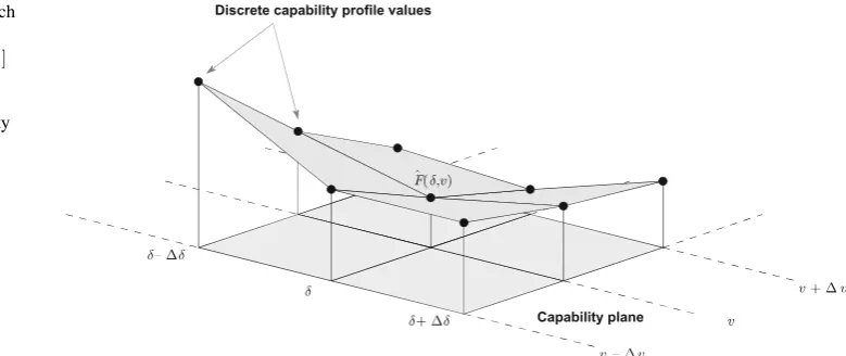
Recall from Sect.3.2 and the original publication [12] that a capability profile is represented by a set of samples. As illustrated in Fig.8, the samples correspond to predeter-mined, discrete values of the load’s position and velocity i.e. a regular, dense mesh over the capability plane. As explained earlier in this section, only those samples which lie on the paths of set-ending repetitions are directly measured. To estimate the values of the capability profile corresponding to regions enclosed by the paths, interpolation using a quadratic form penalty was performed. Formally, the discrepancy in the values of the capability profile of two samples neigh-bouring in thedor position direction is computed as:

DJd ¼kd F^ðd;vÞ F^ðdþDd;vÞ

2

: ð33Þ

Similarly, for samples neighbouring in thevor velocity direction is:

DJv¼kv F^ðd;vÞ F^ðd;vþDvÞ

2

; ð34Þ

and finally in the diagonal direction:

DJdv¼kdvF^ðd;vÞ F^ðdþDd;vþDvÞ

2

; ð35Þ

Thus, the full error functionJwhich is minimized is:

J¼ X

dmaxDd

d¼0 Xvmax

v¼0

kdF^ðd;vÞ F^ðdþDd;vÞ

2

þX

dmax

d¼0 X

vmaxDv

v¼0

kv F^ðd;vÞ F^ðd;vþDvÞ

2

þ X

dmaxDd

d¼0 X

vmaxDv

v¼0

kdvF^ðd;vÞ F^ðdþDd;vþDvÞ

2

:

ð36Þ

As the form of J is quadratic, minimization over unknown values of the capability profile samples is com-puted readily in closed form by differentiation.

Fig. 8 Capability profile which is a bivariate functionF^ðd;vÞ

overd2 ½0;dmax,v2 ½0;vmax

is represented by a set of samples taken from a regular dense mesh over the capability plane. Load displacement is thus constrained to discrete values 0 iDd dmax and

velocity to 0 jDv vmaxfor

Cross-Validation and Empirical Results

In this paper we introduced a cascade of algorithms which allow for an athlete’s capability profile to be estimated from the athlete’s resistance training performance captured in video form. Our methods need only minimal human input and allow for the use of realistic and virtually unconstrained video sequences. Thus, little technical proficiency from the user is required. We finish this section with an empirical demonstration of how the underlying capability profile representation together with the algorithms developed in the present work allows for accurate and principled prediction of performance under unseen conditions.

Design

The effectiveness of the proposed method was evaluated using the video footage of 12 trainees, 10 male and 2 female, performing multiple sets of the squat or the bench press. All of the participants had been regularly performing the corresponding exercise for at least the last 5 years. The participants’ mean age and bodyweight were, respectively, 32.8 years and 91.6 kg, and the corresponding standard deviations 6.0 years and 15.0 kg. The squat and the bench press were chosen as exercises used by a wide range of trainees with different goals, and which can be safely performed to momentary muscular failure1both at low and high intensities (from 15RM to 3RM in our case). After a gradual warm-up, during which the athlete followed his/her established routine, maximum 15RM, 12RM and 8RM lifts were recorded for the training of our algorithm (i.e. learning the athlete’s capability profile) and a 3RM lift for validation purposes. Notice that in practice, by ensuring consistent monitoring of performance (for discussion see Sect.4), a far larger amount of data would be available for the capability profile estimation.

Capability Profile Estimation

In the case of all video sequences used for the evaluation herein, the camera angle was not in any way specially chosen (e.g. to capture either the fully frontal or the fully profile view of the trainee). As desirable in practice, the camera was instead simply placed in a location which was found to be convenient in the context of the equipment setup of the training facility.

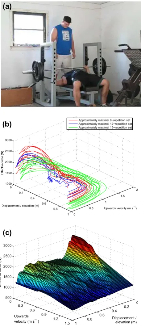
A typical keyframe of one of the videos used to extract training and validation data used to evaluate the proposed methods is shown in Fig.9a. The corresponding charac-teristics of the training lifts are shown in Fig.9b. Note that

the remarkable resemblance of the characteristics of dif-ferent repetitions in the same set supports our fatigue management model introduced in Sect. 3.3.2. Under the maximum exertion model used in [12] (reviewed in Sect.3.3), greater effects of accumulating fatigue would

(a)

(b)

(c)

Fig. 9 a A snapshot from the video used to collect data for the evaluation of the methods introduced in this paper,bthe variation in effective force exerted by the athlete against the load through repetitions of sets at different loading intensities and cthe corre-sponding capability profile reconstruction

have been expected. A reconstruction of the athlete’s capability profile is shown in Fig.9c.

Comparison with Measured Performance

The main results of our experiment are summarized in Fig.10a which shows the plot of predicted 3RM loads against those that were determined empirically. In the case of perfect prediction, the data points would lie on the dotted line shown in the plot. While our algorithm expectedly did not attain perfect performance, it is readily apparent that it has performed remarkably well. Specifically, the measured

standard deviation of the prediction error was found to be 3.7% for the squat and 3.4% for the bench press. This compares favourably with the well-known Brzycki equa-tion [41, 42], for example, particulary considering that empirically obtained maximum strength estimates from higher repetition ranges (such as those used here) exhibit greater test–retest variability [43–45].

While a comparison of maximum effort lifting perfor-mances predicted using statistical, regression techniques and that using the model proposed in the present paper allows for clear and readily understood validation of the information extracted as a capability profile, the capability profile model is much richer in information, allowing for a far wider spectrum of predictions to be cast. To exemplify this, here we also show an example of a comparison between the actual, empirically measured performance characteristics with those simulated using the capability profile estimate of Sect. 3.4.2.

Actual lifting performance characteristics were collected by asking the trainee to perform the maximum number of repetitions using a 3RM load which was previously deter-mined to be 375 lbs. From a video recording of the lift, the elevation and velocity of the load through time were then extracted using the methods described in Sect.3.1. Finally, a comparison was made with performance simulated using the capability profile of Sect.3.4.2. The result of this compar-ison is summarized on the graph shown in Fig.10b. Lifting characteristics predicted by the model described in this paper match the measured motion of the load remarkably well throughout the entire duration of the lift i.e. across all three repetitions. It is particularly interesting to observe that the model correctly predicted even subtle phenomena such as small convexities and concavities in the elevation–time plots of Fig.10b. The convexities and concavities likely correspond to loci in the exercise range of motion (ROM) when a transition, respectively, from a biomechanically weaker to a biomechanically stronger or a biomechanically stronger to a biomechanically weaker position of the load occurs. That performance characteristics of this nature are predicted with such precision provides strong evidence that the underlying model is capable of accurately capturing those elements of the athlete’s fitness which govern relevant exercise performance, as well as that the proposed methodology for inferring the parameters of the model is indeed extracting meaningful information from training data.

Application in Training Analysis and Design

Owing to the central role that the capability profile plays, the ability to estimate it from actual performance opens a wide range of possibilities for practical use. To illustrate

(a)

(b)

this, we developed a computer application that allows a practitioner to investigate predicted athlete-specific effects of differently targeted training regimes. The key aspects of the application’s functionality are described next.

Summary of Software Features

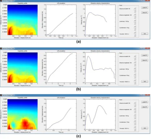
Figure11a shows the main window of the software and its principal elements. The window consists of four panels

and a selection of buttons controlling the application. The panel furthest to the left is the Capability Profile Panel which displays the capability profile which is studied. Furthest to the right is the Exercise Setup Panel con-taining controls that adjust a variety of exercise parame-ters (that are not already implicitly incorporated in the capability profile). The central two panels display simu-lated performance characteristics (as in Sect.3.4.3), pre-dicted by using the capability profile shown in the Capability Profile Panel and resistance variables from the

Fig. 11 Main window of the software demonstrating a possible practical application the methods proposed in this paper. a The capability profile from Fig.9c displayed as acolour-coded imageand the predicted performance characteristics for the values of resistance

Exercise Setup Panel. The first of the central panels shows predicted performance as a plot of the load’s ele-vation against time; the other panel shows the same data but in the form of the corresponding capability plane path (the reader may find it useful to revisit the material of Sect.3.1 as well as [12]).

Capability Profile Panel

The left-most panel in the main window of our software application shows the capability profile, displayed as an image. The rate of force production at a particular com-bination of values of the load’s elevation and velocity is indicated using a colour-code, with warmer colours cor-responding to higher force and cooler colours to lower force, see Fig.11a. Note, for example, that the top of the image is uniformly blue corresponding to diminished capability to exert force against a rapidly moving load.

The capability profile, which may have been estimated using the algorithm described in the previous sections, can be modified by the user. Clicks in the capability plane with the left and right mouse buttons produce, respectively, positive and negative Gaussian ‘‘bumps’’ in the profile. Formally, a click at the location corre-sponding to ðx0;v0Þ creates a modified profile F^modðd;vÞ

from F^ðd;vÞ: ^

Fmodðd;vÞ ¼F^ðd;vÞ þmGðd0;v0;rd;rvÞ; ð37Þ

wheremis the adjustable (see next paragraph) magnitude of the effect, while parametersrdandrv, which too are user-adjustable, control its breadth in the capability plane. This principle of capability profile modification is similar to that described in detail in [35].

The example in Fig.11c shows the resulting capa-bility profile after the original one from Fig.11a was modified by decrementing the force in the locality of the point of elevation-velocity ðd;vÞ ð0:2 m;0:45 m s1_Þ

and incrementing it in the locality of ðd;vÞ ð0:6 m;0:6 m s1_Þ.

Exercise Setup Panel

The panel furthest to the right in the main window of our application is the Exercise Setup Panel, used to control a number of exercise parameters. The first two of these control the effects of user input. ‘‘Influence breadth’’, changes the width of the capability profile modification (relative to the scale d2 ½0;dmax;v2 ½0;vmaxof the

ele-vation–velocity plane region displayed) affected by input: rd¼ ðinfluence breadthÞ dmax ð38Þ

rv¼ ðinfluence breadthÞ vmax ð39Þ

‘‘Influence magnitude’’ controls the magnitude mof the adjustment in Eq.37. The remaining three parameters con-trol the nature of resistance used to predict performance characteristics achieved when the current capability profile is used in a computer simulation of a lifting effort. To account for different types of resistance commonly encountered in weight training equipment we consider the general mechanism schematically illustrated in Fig. 12. Thus, ‘‘load mass‘‘ is the massmof the free adjustable load, such as a weighted barbell, while ‘‘countermass’’ m0 and

‘‘viscosity’’care, respectively, the mass of a counterweight and the viscous resistance constant. An unmodified, free weight lift, is obtained by settingm0¼0 andc¼0.

Legend:

g acceleration due to gravity

m mass of the adjustable load

m0 mass of the counterweight

x₁,x2 displacements of the adjustable load and the counterweight ˙

x₁ velocity of the adjustable load

T cord tension (T≥0)

c viscous resistance

F_f1,Ff2 friction forces.

Fig. 12 A schematic diagram of the key components of the resistance mechanism considered in the present work. Forces acting on the system when the direction of the velocity of both the adjustable load

Predicted Performance Panels

The central two panels of the main window hold plots of, respectively, the variation of the load’s elevation as a function of time and the path of the elevation–velocity state vector in the capability plane through the lift. These are estimated using a computer simulation as described in [35], performed automatically after any of the application parameters are changed: the capability profile or the resistance settings.

Discussion

Having described the key aspects of our software’s func-tionality, we lastly describe how such a computer tool may be used in day to day training practice.

The challenge central to the design of a continuously productive training regime is that of feedback-based adjustment of training parameters. In principle, the under-lying idea is simple and consists of the following stages:

Step 1: Observation Actual performance in training is monitored (usually by a coach or the athlete himself) and compared with the projected performance.

Step 2: Limiting factor identification

Aspects of performance which are assessed to be the limiting factors in progress are identified.

Step 3: Parameter adjustment

A suitable modification of training parameters is implemented to correct for the weaknesses identified in Step 2.

Observation: data acquisition It has been emphasized throughout this paper that one of our key aims is to develop a principle system for monitoring, evaluating and optimizing training which is inexpensive and convenient, requiring little technical proficiency from the user. Indeed the proposed methods require no more than a readily affordable camera and a PC. One of the consequences of a setup such as this is that training data can be continuously acquired, allowing for the creation of a more reliable and up-to-date model of an athlete’s fitness. Specifically, video sequences (acquired by the athlete’s coach, training part-ner or using a stationary camera set up by the athlete himself) of the athlete’s training sets can be continuously fed into our capability profile estimation algorithm (see Sect.3).

Limiting factor identification: performance analysis The task of identifying those aspects of an athlete’s fitness which are limiting performance is usually not trivial. This is because unlike the task of observing past performance, here it is necessary to be able tohypothesizesmall changes

to specific aspects of the athlete’s fitness and furthermore

predict the nature and magnitude of performance change they would produce. The software tool described at the beginning of this section achieves precisely this in the context of resistance training. Guided by insight and experience, the coach can investigate how small changes to the athlete’s current capability profile affect performance. For example, a ready estimate of the new maximum strength can be obtained. Alternatively, different training modalities can be explored. By changing the loading parameters, the practitioner can promptly see how this is reflected on the corresponding path in the capability plane i.e. which aspects of performance are exerted and trained the most.

Parameter adjustment The adjustment of training parameters to achieve performance improvement is inti-mately linked to the previously discussed task of identi-fying those aspects of fitness which currently limit performance. This link is made explicit in our model and software. A productive adjustment is one which directs capability paths of training repetition sets towards capa-bility plane regions which correspond to limiting force production conditions. This can be achieved by the prac-titioner though experimentation with loading parameters in the Exercise Setup Panel and observation of the effects on training performance characteristics. It is worth noting the indispensability of experience and insight, that is to say the human factor, in guiding such experimentation.

Summary and Conclusions

The work described in this paper addressed a broad range of practical challenges which until now limited the appli-cation of a recently proposed model of neuromuscular adaptation to resistance training. In a number of studies this model has demonstrated promising results both in predic-tive and explanatory domains, and revealed novel insights into different training practices. Being able to take this model, or indeed future models based upon similar pre-mises, from the realm of theoretical or highly specific studies and make them useful in everyday practice has the potential of transforming the use of technology in sports and of reshaping sports science research.

Starting from raw video input, acquired using readily available, low cost equipment, the proposed framework consists of a series of steps, ending with an estimate of the parameters of the model describing a specific athlete’s force production capability in a given exercise. The key contributions include:

• robust estimation of the position, velocity and acceler-ation of the load,

• effective force estimation from the characteristics of the load’s motion,

• a model of force–fatigue management applicable to the trained population

• inference of the athlete’s maximum force production capability at a certain position in a lift from the estimate of the effective force actually exerted, and

• reconstruction of the relevant regions of the capability profile from curved cross-sections through the capabil-ity profile.

The proposed framework was evaluated empirically using data representative of that which would be used in weight training practice. Agreement of the model’s predictions with empirical performance data and relevant previous work was demonstrated. Finally, a description of a software program implementing the proposed framework was used to illustrate its possible application in practice as a tool for monitoring, evaluating and improving training performance.

Compliance with Ethical Standards

Conflict of interest On behalf of all authors, the corresponding author states that there is no conflict of interest.

Open Access This article is distributed under the terms of the Creative Commons Attribution 4.0 International License (http://creative commons.org/licenses/by/4.0/), which permits unrestricted use, distri-bution, and reproduction in any medium, provided you give appropriate credit to the original author(s) and the source, provide a link to the Creative Commons license, and indicate if changes were made.

References

1. Cardinale M, Erskine JA (2008) Vibration training in elite sport: effective training solution or just another fad? Int J Sports Physiol Perform 3(2):232–239

2. Abe T, Kearns CF, Sato Y (2006) Muscle size and strength are increased following walk training with restricted venous blood flow from the leg muscle, kaatsu-walk training. J Appl Physiol 100(5):1460–1466

3. Swinton PA, Lloyd R, Agouris I, Stewart A (2009) Contemporary training practices in elite British powerlifters: survey results from an international competition. J Strength Cond Res 23(2):380–384 4. Robbins DW, Young WB, Behm DG, Payne WR (2010) The effect of a complex agonist and antagonist resistance training protocol on volume load, power output, electromyographic responses, and efficiency. J Strength Cond Res 24(7):1782–1789 5. Krieger JW (2010) Single vs. multiple sets of resistance exercise for muscle hypertrophy: a meta-analysis. J Strength Cond Res 24(4):1150–1159

6. Caruso JF, Coday MA (2008) The combined acute effects of massage, rest periods, and body part elevation on resistance exercise performance. J Strength Cond Res 22(2):575–582 7. Zainuddin Z, Newton M, Sacco P, Nosaka K (2005) Effects of

massage on delayed-onset muscle soreness, swelling, and recovery of muscle function. J Athl Train 40(3):174–180

8. Sharp DR, Pearson CP (2010) Amino acid supplements and recovery from high-intensity resistance training. J Strength Cond Res 24(4):1125–1130

9. Colado JC, Garcı´a-Masso´ X (2009) Technique and safety aspects of resistance exercises: a systematic review of the literature. Phys Sportsmed 37(2):104–111

10. Fithian DC, Powers CM, Khan N (2010) Rehabilitation of the knee after medial patellofemoral ligament reconstruction. Clin Sports Med 29(2):283–290

11. Arandjelovic´ O (2013) Computer simulation based parameter selection for resistance exercise. Model Simul 24–33

12. Arandjelovic´ O (2010) A mathematical model of neuromuscular adaptation to resistance training and its application in a computer simulation of accommodating loads. Eur J Appl Physiol 110(3):523–538

13. Zatsiorsky VM (1995) Science and practice of strength training. Human Kinetics, Windsor

14. Komi P (1979) Neuromuscular performance: factors influencing force and speed production. Scand J Sports Sci 1:2–15 15. Smith LK, Weiss EL, Lehmkuhl LD (1996) Brunnstrom’s clinical

kinesiology, 5th edn. F.A. Davis Company, Philadelphia 16. Hill AV (1953) The mechanics of active muscle. Proc R Soc

Lond B Biol Sci 141:104–117

17. Perrine JJ, Edgerton VR (1978) Muscle force-velocity and power-velocity relationships under isokinetic loading. Med Sci Sports 10(3):159–166

18. Caiozzo VJ, Perrine JJ, Edgerton VR (1981) Training-induced alterations of the in vivo force-velocity relationship of human muscle. J Appl Physiol 53(3):750–754

19. Lowe DG (2003) Distinctive image features from scale-invariant keypoints. Int J Comput Vis 60(2):91–110

20. Harris C, Stephens M (1988) A combined corner and edge detector. In: Proceedings of Alvey vision conference, pp 147– 151

21. Lucas BD, Kanade T (1981) An iterative image registration technique with an application to stereo vision. In: Proceedings of international joint conference on artificial intelligence (IJCAI), pp 674–679

22. Tomasi C, Kanade T (1991) Detection and tracking of point features. Carnegie Mellon University Technical Report CMU-CS-91-132

23. Shi J, Tomasi C (1994) Good features to track. In: Proceedings of IEEE conference on computer vision and pattern recognition, pp 593–600

24. Martin R, Arandjelovic´ O (2010) Multiple-object tracking in cluttered and crowded public spaces. In: Proceedings of inter-national symposium on visual computing, vol 3, pp 89–98 25. Arandjelovic´ O (2011) Contextually learnt detection of unusual

motion-based behaviour in crowded public spaces. In: Proceed-ings of international symposium on computer and information sciences, pp 403–410

26. Arandjelovic´ O (2015) Automatic vehicle tracking and recogni-tion from aerial image sequences. In: Proceedings of IEEE con-ference on advanced video and signal based surveillance, pp 1–6 27. Kitai TA, Sale DG (1989) Specificity of joint angle in isometric

training. Eur J Appl Physiol Occup Physiol 58(7):744–748 28. Knapik JJ, Mawdsley RH, Ramos MU (1983) Angular specificity

and test mode specificity of isometric and isokinetic strength training. Eur J Appl Physiol Occup Physiol 5(2):58–65 29. Kompf J, Arandjelovic´ O (2016) Understanding and overcoming

the sticking point in resistance exercise. Sports Med. doi:10.1007/ s40279-015-0460-2

31. Alonso FJ, Cuadrado J, Lugrı´s U, Pintado P (2010) A compact smoothing-differentiation and projection approach for the kine-matic data consistency of biomechanical systems. Multibody Syst Dyn 24(1):67–80

32. Silva MPT, Ambro`sio JAC (2002) Kinematic data consistency in the inverse dynamic analysis of biomechanical systems. Multi-body Syst Dyn 8(2):219–239

33. de Boor C (1978) A practical guide to splines. Springer, Berlin 34. Neelly K, Carter SA, Terry JG (2010) A study of the resistive

forces provided by elastic supplemental band resistance during the back squat exercise: a case report. J Strength Cond Res 24(supplement):1

35. Arandjelovic´ O (2011) Optimal effort investment for overcoming the weakest point: new insights from a computational model of neuromuscular adaptation. Eur J Appl Physiol 111(8):1715–1723 36. Arandjelovic´ O (2012) Common variants of the resistance mechanism in the Smith machine: analysis of mechanical loading characteristics and application to strength-oriented and hyper-trophy-oriented training. J Strength Cond Res 26(2):350–363 37. Arandjelovic´ O (2013) Does cheating pay: the role of externally

supplied momentum on muscular force in resistance exercise. Eur J Appl Physiol 113(1):135–145

38. Behm DG, Sale G (1993) Velocity specificity of resistance training. Sports Med 15(6):374–388

39. Shimano T, Kraemer WJ, Spiering BA, Volek JS, Hatfield DL, Silvestre R, Vingren JL, Fragala MS, Maresh CM, Fleck SJ, Newton RU, Spreuwenberg LP, Ha¨kkinen K (2006) Relationship between the number of repetitions and selected percentages of one repetition maximum in free weight exercises in trained and untrained men. J Strength Cond Res 20(4):819–823

40. Cormen TH, Leiserson CE, Rivest RL (1990) Introduction to algorithms. MIT Press, Cambridge

41. Brzycki M (1993) Strength testing: Predicting a one-rep max from a reps-to-fatigue. J Phys Ed Recreat Dance 64(1):88–90 42. Brzycki M (1998) A practical approach to strength training.

McGraw-Hill, New York

43. Stock MS, Beck TW, DeFreitas JM, Dillon MA (2011) Test-retest reliability of barbell velocity during the free-weight bench-press exercise. J Strength Cond Res 25(1):171–177

44. Materko W, Santos EL (2009) Prediction of one repetition maximum strength (1rm) based on a submaximal strength in adult males. Isokinet Exerc Sci 17(4):189–195