An experiment to assess the effects of diatom dissolution on oxygen isotope ratios

An experiment to assess the effects of diatom dissolution on oxygen isotope ratios

Andrew C. Smitha*, Melanie J. Lenga,b, George E.A. Swannb,c, Philip A. Barkerd, Anson W. Mackaye, David B. Ryvesf, Hilary J. Sloanea, Simon R.N. Cheneryg, Mike Hemsh

a _{NERC Isotope Geosciences Facilities, British Geological Survey, Nottingham, NG12 5GG} b

Centre for Environmental Geochemistry, University of Nottingham, Nottingham, NG7 2RD c _{School of Geography, University of Nottingham, University Park, Nottingham, NG7 2RD} d

Lancaster Environment Centre, Lancaster University, Lancaster, LA1 4YQ

e _{Environmental Change Research Centre, Department of Geography, UCL, London WC1E 6BT} f _{Centre for Hydrological and Ecosystem Science (CHES), Department of Geography, Loughborough}

University, Loughborough, LE11 3TU

g _{British Geological Survey, Keyworth, Nottingham NG12 5GG} h _{Department of Geology, University of Leicester, Leicester, LE1 7RH}

* Corresponding author: email andrews@bgs.ac.uk; phone +447970359920

Abstract

Rational: Current studies which use the oxygen isotope composition from diatom silica

(Odiatom) as a palaeoclimate proxy assume that Odiatom reflects the isotopic composition

of the water in which the diatom formed. However, diatoms dissolve post mortem,

preferentially losing less silicified structures in the water column and during/after burial into

sediments. The impact of dissolution on Odiatom and potential misinterpretation of the

palaeoclimate record is evaluated.

Methods: Diatom frustules covering a range of ages (6 samples from the Miocene to the

Holocene), environments and species were exposed to a weak alkaline solution for 48 days at

two temperatures (20ºC and 4ºC), mimicking natural dissolution post mucilage removal.

Following treatment, dissolution was assessed using Scanning Electron Microscope images

and a qualitative diatom dissolution index. Diatoms were subsequently analysed for O using Step Wise Fluorination and Isotope Ratio Mass Spectrometry.

Results: Variable levels of diatom dissolution were observed between the 6 samples, in all

cases higher temperatures resulted in more frustule degradation. Dissolution was most

evident in younger samples, likely as a result of the more porous nature of the silica. The

degree of diatom dissolution does not directly equate to changes in isotope value; Odiatom

was however lower after dissolution, but in only half the samples was this reduction outside

the analytical error (2σ analytical error = 0.46‰).

Conclusions: We show that dissolution can have a small negative impact on Odiatom

causing reductions of up to 0.59‰ beyond analytical error (0.46‰) at natural environmental

temperatures. These findings need to be considered in palaeoenvironmental reconstructions

using Odiatom, especially when interpreting variations in Odiatom of <1‰.

Keywords: Palaeoclimate, biogenic silica, oxygen isotopes, dissolution, sedimentation

Introduction

Use of the oxygen isotope composition of biogenic silica (most often diatom silica; Odiatom)

in palaeoclimate reconstructions from both lake and ocean studies is increasing.[1,2] Diatom



O offers an alternative to more traditional carbonate O analysis, especially in environments where carbonates are not well preserved. For example, Pike et al., (2013)[3]

used Odiatom to reconstruct the amount of melting along the Antarctic Peninsula through the

Holocene, and Mackay et al., (2013)[4] use Odiatom from Lake Baikal to understand the

extent of Northern Hemisphere climate forcing over central Asia during the Last Interglacial.

These studies assume that the Odiatom is fixed in the frustules during formation and that the

signal is not subsequently altered post mortem by interactions with isotopically different

fluids, or by dissolution, either during sinking or in the sediments. This assumption, however,

is inconsistent with kinetic theory, as equilibrium is dynamic, and mass transfer continues at

the mineral-fluid interface even after the diatom frustule attains equilibrium with the bulk

fluid. This is especially pertinent to biogenic silica because of its hydrous nature

(SiO2.nH2O).[5,6]

The aim of the experiments reported here was to assess the impact of post mortem biogenic

causing the component of the frustule that remains to be only partially representative of the

original.[8] We questioned if the isotope composition of the frustule may change through dissolution due to removal of the most easily dissolved components in diatoms of different

age. One laboratory dissolution experiment (at pH 9 using NaOH) carried out by Moschen et

al., (2006)[9] on modern diatoms observed isotope deviations of up to 6.9‰ due to dissolution, following the removal of the protective organic matter coating around the

cultured frustule, whereas Dodd et al. (2012)[6] report a 7‰ shift from living to sedimentary diatoms, related to silicate maturation. To test more fully if such extreme fractionation may

occur due to post burial dissolution (assessed by a visual dissolution index; c.f. Ryves et al.,

2006[10]), we carried out further experiments. We mimicked dissolution in the laboratory on a suite of monospecific and mixed diatom assemblage of different ages, from both marine and

lacustrine environments, and dissolved them to different degrees over varying time and at two

temperatures.

Previous Studies

Diatom dissolution experiments have previously been undertaken to assess structural changes

in community composition[11,12,13] and alteration of oxygen and silicon isotope ratios[7,9] using a variety of reagents. These studies demonstrate that the removal of organic components and

metal ions greatly accelerates dissolution through contact between the solution and the silica

structure.[9] Even after the removal of the organic coating, Ryves et al., (2001)[13] found that partial dissolution took several weeks when conducted in distilled water at 25ºC buffered to

pH 10. Dissolution rates are affected by several factors, including the silica concentration of

the solution, pH and temperature of the solution[13] as well as the amount of diatom silica remaining and the proportion of this silica which is resistant to dissolution.[9] In natural sediments pore water chemistry is more important than ambient lake water conditions and

dissolution is often greater in more open sediment structures. However, Flower & Ryves

(2009)[14] found that preservation is better (i.e. less dissolution) at higher sediment

accumulation rates and suggested this was due to rapid burial and build-up of silica saturation

levels in pore water.

Bulk dissolution rate in sediments is therefore not linear but decreases over time,[7,15] both as pore water concentrations rise to saturation but also as the assemblage specific surface area is

while the rate decreases in older sediments as a result of greater crystallinity in older

diatoms.[16] At the scale of individual valves specific surface area is also important to dissolution rates, as valves dissolve their surface area to volume ratio changes altering the

rate of dissolution.[12,13] Finally, the ultra-structure of the diatom frustule can also have significant effects on the rate of dissolution as susceptibility to dissolution is not uniform

across the valve. Within the silica ultra-structure of the valve, a variety of bond geometries

exist. Specifically the arrangement of silica and oxygen atoms may be denoted by Qn, where

n denotes the number of silicon atoms connected to four bridging oxygen atoms.[17] For

example Q4 denotes a silicon atom joined to four other silicon atoms via four bridging

oxygen atoms (i.e. Si(OSi)4). Q3 therefore denotes a silicon atom connected to three other

silicon atoms via three bridging oxygen atoms, with the fourth oxygen forming a hydroxyl

group (i.e. (SiO) Si-OH). The majority of bonds present are typically either Q4 or Q3, leading

to the ratio Q4/Q3 being quoted to indicate the hydration level.[17] Importantly, a higher Q4/Q3

ratio gives a silica structure more resistance to dissolution, owing to the lower bond energy of

the hydroxyl groups compared to the Si-O-Si bonds.[18]

Previous studies have tried to explain post mortem Odiatom variation, looking specifically at

the effects of dissolution.[9,19] The study of Moschen et al., (2006)[9] involved sediment traps

in Lake Holzmaar, Germany, to investigate changes in Odiatom during settling at different

water depths (0-7 m and 20 m). Their results show an increase in Odiatom with depth,

associated primarily with the re-suspension of older diatoms which had undergone significant

levels of silicate maturation. Importantly, subsequent laboratory experiments conducted using

buffered (pH 5.6 and pH 9) solutions and both cultured and natural diatoms (untreated, and

cleaned of organic coatings using H2O2) found a Odiatom increase of up to +6.9‰ after two

days at pH 9,[9] although no change was found in Odiatom in the lower pH solution. In the

untreated samples, where the organic mucilage was retained, they found limited dissolution

of biogenic silica and no oxygen isotope change.[9] The natural diatom assemblage underwent very little dissolution in comparison to the cultured diatoms, the “older” natural diatoms

being more resilient to both dissolution and Odiatom change.[9,19] These results highlight the

potential importance of dissolution in controlling Odiatom in diatom assemblages of

different ages.

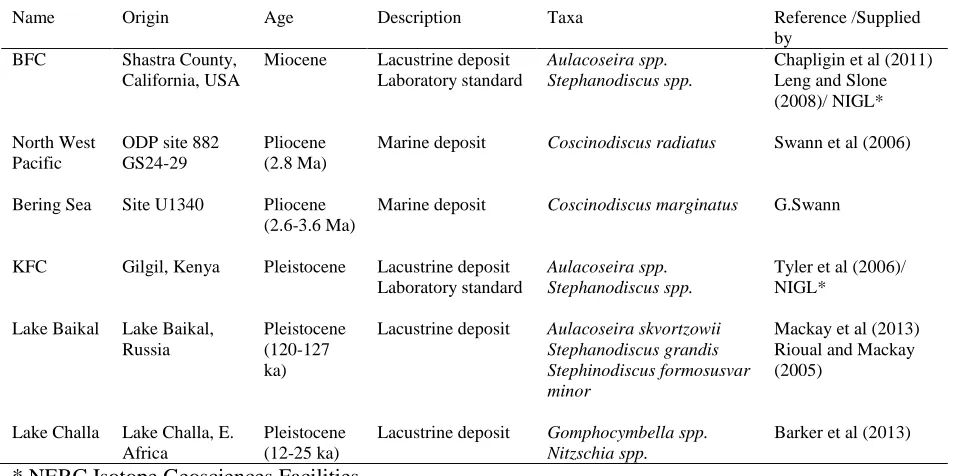
Six samples were selected (most of which had been previously analysed for Odiatom, Table

1) that cover a range of sedimentary environments and species composition. From oldest to

youngest, these were: 1) Burney California Diatomite (BFC) (Miocene lacustrine deposit), 2)

North West Pacific Ocean (Pliocene marine deposit), 3) Bering Sea (Pliocene marine

deposit), 4) Gil-Gil Kenya Diatomite (KFC) (Pleistocene lacustrine deposit), 5) Lake Baikal

(Pleistocene lacustrine deposit), 6) Lake Challa (Pleistocene lacustrine deposit). All these

samples would have undergone an unknown amount of prior dissolution during settling and

burial. The samples had been previously cleaned and prepared for isotope analysis which

removed any carbonate or siliclastic particles but also removed any remaining organic

components (see original publications in Table 1). The six samples were sieved and cleaned

of silt material until they contained over 90% diatom silica (visually assessed using either a

Scanning Electron Microscope and/or a light microscope), with the exception of KFC which

contained a significant proportion of clay which could not be removed during processing, and

the Bering Sea sample, which contained up to 15% sponge spicules which were similar in

size and density to the diatoms (see original publications in Table 1).

Name Origin Age Description Taxa Reference /Supplied

by

BFC Shastra County,

California, USA

Miocene Lacustrine deposit Laboratory standard

Aulacoseira spp. Stephanodiscus spp.

Chapligin et al (2011) Leng and Slone (2008)/ NIGL*

North West Pacific

ODP site 882 GS24-29

Pliocene (2.8 Ma)

Marine deposit Coscinodiscus radiatus Swann et al (2006)

Bering Sea Site U1340 Pliocene (2.6-3.6 Ma)

Marine deposit Coscinodiscus marginatus G.Swann

KFC Gilgil, Kenya Pleistocene Lacustrine deposit Laboratory standard

Aulacoseira spp. Stephanodiscus spp.

Tyler et al (2006)/ NIGL*

Lake Baikal Lake Baikal, Russia

Pleistocene (120-127 ka)

Lacustrine deposit Aulacoseira skvortzowii Stephanodiscus grandis Stephinodiscus formosusvar minor

Mackay et al (2013) Rioual and Mackay (2005)

Lake Challa Lake Challa, E. Africa

Pleistocene (12-25 ka)

Lacustrine deposit Gomphocymbella spp. Nitzschia spp.

Barker et al (2013)

* NERC Isotope Geosciences Facilities

The six samples were either near-monospecific or mixed diatom assemblages, the dominant

species composition for each sample is summarised in Table 1. Prior to dissolution

experiments, a subsample of each was analysed for δ18

O. Further subsamples (25 mg) were

placed in a 5% NaCO3 solution (250 ml, made up with deionised water, δ18O = –7 ‰, pH c.

11.5) to ensure silica did not become oversaturated during the experiment and to mimic

natural dissolution post mucilage removal.[20] Dissolution was allowed to proceed for 48 days at two temperatures (20°C and 4°C) representing a range of temperatures including low

temperatures found within bottom waters (and therefore sediments) of high latitude lakes and

the oceans. The samples were kept in beakers with para film coverings to prevent evaporation

and the samples were not stirred; the 20ºC experiment was conducted in a fume cupboard and

the 4ºC in a fridge. A control subsample was taken from three of the diatom assemblages

(BFC, North West Pacific and Bering Sea) and placed in de-ionised (DI) water for the 48 day

period (pH c.7, 20ºC). The reactions were halted by filtering onto cellulose nitrate filters

(3µm), washing in deionised water and drying at 40oC. To ensure that changes in Odiatom

are not related to different rates of dissolution between species, qualitative assessment of

diatom composition before and after dissolution was assessed using both light (LM) and

scanning electron microscopes (SEM) and only minor changes in assemblage composition

were identified, potentially related to heterogeneity across the viewing surface of the slide.

For SEM imaging, samples were mounted on carbon tipped aluminium stubs and to achieve a

better image quality, the samples were coated with gold using an Emitech K500X manual

sputter coater. The coated stubs were subsequently imaged under an Hitachi S-3600N

Scanning Electron Microscope, with a working distance of 15 mm and voltage of 15 Kv. The

relative change in diatom dissolution state was then assessed for the dominant taxa in each

sample using the dissolution stage classification of Ryves, (1994)[21] and the Diatom Dissolution index (DDI),[10,22] Equation 1.

𝐷𝐷𝐼 =∑𝑠=4𝑠=1𝑛𝑠·(𝑆−1)

𝑁·(𝑆𝑚𝑎𝑥−1) (Eq 1)

Where n is the number of valves and S represents the stage of valve dissolution, N is the total

number of classified valves. Smax is the highest stage that valves in the assemblage could

reach if dissolution progressed to its end point; Smax thus varies between 2 and 4,[10] and here

was 3 in all cases (see Table 2). The DDI enables the user to estimate the proportion of valves

numerical value for sample dissolution, with 0 indicating perfect preservation and 1

indicating the maximum dissolution possible for that species or assemblage if all species are

included in the dissolution assessment[10]. Within each sample an area containing at least 100 valves of the dominant species was imaged (between 500 and 600x magnification), two

additional images at the same magnification were subsequently taken to verify the initial DDI

count. Although only the most important species (by relative abundance) were assessed for

dissolution (Table 2), the DDI based on dominant taxa is a good estimate of assemblage DDI,

which is a weighted mean of individual species DDIs. Similarly, while all biogenic silica

contributes to sample δ18

O, in these samples the dominant taxa account for most of the

biogenic silica (by biovolume). Dissolution stages for the dominant taxa (Table 2) were

initially established by comparison to dissolution sequences published for the same genus

and/or morphology[22] and refined for each dominant taxon by identification of repeatable and distinct patterns in the valves under SEM/LM.

Stage 1 Stage 2 Stage 3

Coscinodiscus

spp.

Girdle completely intact. Almost all areolae have vela intact. Almost all

cellular mantle areolae have vela

intact.

Most central areolae have lost vela and become enlarged. Some cellular

mantle areole vela have been lost.

Girdle almost completely intact.

Almost all areolae vela are lost, including all cellular mantle areolae

vela. Girdle beginning to break

down as areolae begin to coalesce.

Gomphocymbella

spp.

Striae lineations clear and well

preserved, puncta intact and mantle

well preserved. Hypotheca and

epitheca still together.

Puncta enlarged, with dissolution

beginning at ends of frustule.

Hypotheca and epitheca may

separate, although not in this image.

Epitheca and hypotheca typically

separated, with only the costae

remaining. Commonly seen as ‘skeleton’ type remains.

Aulacoseira

skvortzowii

Mantle completely intact. Areole not enlarged, vela present on some

species. No obvious signs of

dissolution.

Areolae beginning to enlarge and coalesce. No vela present. Holes

may become apparent as the areole

begin to coalesce more.

Breakdown of frustule as areole coalesce more completely. Frustule

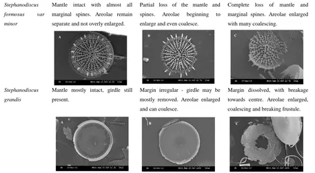
Stephanodiscus

formosus var

minor

Mantle intact with almost all marginal spines. Areolae remain

separate and not overly enlarged.

Partial loss of the mantle and spines. Areolae beginning to

enlarge and even coalesce.

Complete loss of mantle and marginal spines. Areolae enlarged

with many coalescing.

Stephanodiscus

grandis

Mantle mostly intact, girdle still

present.

Margin irregular - girdle may be

mostly removed. Areolae enlarged and can coalesce.

Margin dissolved, with breakage

towards centre. Areolae enlarged, coalescing and breaking frustule.

Table 2: SEM images of diatom dissolution stages for 5 of the prominent taxa recorded in the samples. Frustule degradation associated with dissolution can be clearly identified.

After dissolution, Odiatom was determined using a Step Wise Fluorination (SWF)

technique.[18] The initial SWF stages remove loosely bonded water (dehydration) and hydroxyl using a bromine pentafluoride (BrF5) reagent. The next stage involves a full

reaction at 450ºC for 12 hours with an excess of reagent, causing the dissociation of the silica

into O2 and Si (as SiF4). O2 is then liberated and converted to CO2 by exposure to graphite,

whilst other products of the reaction (SiF4,BrF3) are trapped using liquid nitrogen and either

analysed, e.g. Si, or disposed of.[18] The resultant CO2 gas was then analysed for O using a

Thermo MAT 253 dual inlet isotope ratio mass spectrometer at the Stable Isotope Facility,

British Geological Survey. Sample gas was calibrated against the BFC standard material

which was in turn corrected to NBS28, δ18Odiatom is reported on the VSMOW scale. The DDI and δ18_{O data are given in Table 3 and Figure 2. A 2σ error for the experiment was calculated}

based upon the mean standard deviation of duplicate analysis undertaken on all samples

(including those pre-dissolution, in DI water for 48 days and those dissolved at 20 ºC and 4

ºC for 48 days) and was calculated at 0.46‰, very similar to the 2σ error for repeat analysis of the BFC standard (from all experiments), 0.48‰.

Results

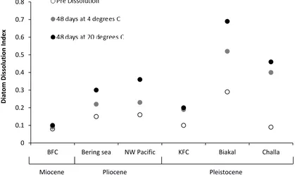
Diatom dissolution was compared before (t = 0) and after the experiments (48 days at 4ºC

and 20ºC) using the Diatom Dissolution Index as defined by Ryves et al., (2009)[22] (Figure 1). Table 2 shows the typical stages of dissolution for major taxa.[22] All diatom samples had a pre-dissolution DDI of 0.1-0.3, while DDI for all samples after 48 days (at both 20ºC and

4ºC) ranged between 0.1 and 0.7 (Figure 1). For all samples, apart from the Miocene aged

BFC, DDI was most extensive after 48 days in the 5% Na2CO3 solution, and in the samples

dissolved at 20ºC (compared to those at 4ºC), similar to results of Demarest et al., (2009).[9]

Figure 1: Diatom Dissolution Index for all samples (in descending age order) under the three different dissolution experiments. Open circles show the DDI pre-dissolution, grey circles after 48 days dissolution at 4ºC and black circles after 48 days at 20ºC.

Isotope composition

The Odiatom composition of the 6 diatom samples was analysed pre-dissolution, after

dissolution for 48 days (at both 20ºC and 4ºC, pH c. 11), and (for comparison) three of the

samples (BFC, North West Pacific and Bering Sea) after 48 days in only deionised water.

Pre-dissolution Odiatom were between +26.92 and +42.79‰ (Figure 2). For the three

samples left for 48 days in DI water, we observed little dissolution under SEM. Change in



Odiatom from pre-dissolution values was within analytical error (0.46‰) for two of the

0 0.1 0.2 0.3 0.4 0.5 0.6 0.7 0.8

BFC Bering sea NW Pacific KFC Biakal Challa

D

iato

m

Di

ssol

u

tion

In

d

e

x

samples (BFC, –0.09‰ and Bering Sea, –0.38‰) but was outside this for the North West

Pacific sample (–0.99‰).

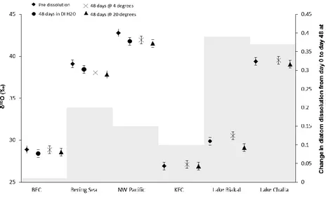
Figure 2: Change in δ18O between pre-dissolution isotope values (diamonds) and the two stages of dissolution, 48 days dissolution at 4ºC (crosses) and 48 days at 20ºC (triangles). Control experiment (48 days in DI water) shown with black circles, error bars denote the analytical error (0.46‰). Change in DDI (grey bars) between pre dissolution values and values after 48 days dissolution at 20ºC.

δ18_O pre-dissolution (‰)

δ18_{O after 48} days at 4ºC (‰)

δ18_{O after 48} days at 20ºC (‰)

DDI pre-dissolution

DDI after 48 days at 4ºC

DDI after 48 days at 20ºC

BFC 28.88 28.86 28.59 0.08 0.09 0.10

NW Pacific 42.79 41.95 41.55 0.15 0.22 0.30

Bering Sea 39.10 38.05 37.84 0.16 0.23 0.36

KFC 26.92 27.11 26.90 0.10 0.19 0.20

Lake Baikal 29.88 30.54 29.12 0.29 0.52 0.69

Lake Challa 39.39 39.54 39.04 0.09 0.40 0.46

Table 3: δ18O and Diatom Dissolution Index data for all samples pre-dissolution, after 48 days at 4ºC and after 48 days at 20ºC. Samples with a δ18_{O change outside of error (0.46‰) are highlighted in} bold.

Of the six samples left to dissolve for 48 days at 4ºC, only the Bering Sea sample (change of

value from the pre-dissolved material outside the sample analytical (2σ) error (average

change in all samples = –0.15‰). The Lake Baikal sample shows a slight (but significant)

increase Odiatom (+0.66‰) at this temperature. All samples from the 48 days at 20ºC

experiment show lower Odiatom, and three exhibit a change outside of analytical error; the

Bering Sea (–1.26‰), NW Pacific (–1.23‰) and Lake Baikal (–0.76‰), with average

change in all samples of –0.65‰ (Figure 2).

Discussion

Diatom dissolution and oxygen isotope fractionation

Isotope change during these experiments is potentially related to two different isotope

fractionation processes. Firstly, the slow equilibrium oxygen isotope exchange between

diatom silica and the surrounding water. This process occurs on the molecular level and takes

a lot of time (or energy) to cause significant isotope exchange; it is therefore unlikely that this

process could cause large changes in Odiatom over the short time period of these

experiments. However, the second form of isotope fractionation is a kinetic process driven by

the preferential dissolution of sections of the diatom frustule. This process occurs far more

rapidly and thus therefore more likely to cause the isotope shifts observed here.

Overall, the diatom dissolution experiments reported here show that, in general, the oldest

diatoms are least affected by further experimental dissolution (Figure 1), as expected as

biogenic silica ages geologically and becomes more crystalline.[5] However KFC (Pleistocene) is an exception, with lower levels of dissolution (DDI change = 0.1), although

this likely still represents a substantial loss of diatoms (perhaps ~30% disappear as DDI rises

from 0.1 to 0.2; see Ryves et al. 2006[10]). This might speculatively be related to clay contamination within the sample. Whilst differences in the extent of diatom dissolution

occurred among the six samples corresponding to the sample age, changes in Odiatom appear

de-coupled from the amount of dissolution (Figure 2 and Table 3). The change in DDI

between assemblages prior to dissolution and after dissolution at 20ºC ranges from 0.01

(BFC) to 0.39 (Lake Baikal), but this variation does not appear related to the Odiatom (linear

regression, n = 6, r2 = 0.04). This dissimilarity between the change in diatom dissolution and the difference in isotope value indicates that there is no overarching relationship between

composition, sample age, the extent of prior diagenetic processing, taphonomic history as

well as preferential dissolution in controlling how Odiatom changes during dissolution.

Whilst the amount of dissolution is not directly related to the change in Odiatom and even

though samples may dissolve in different ways due to their initial assemblage makeup our

results demonstrate that dissolution almost always (one exception) causes a small negative

shift in Odiatom;different from the large positive shifts in Odiatom described in cultured

diatoms.[9] This is potentially because our experiments are an assessment of secondary (within sediment), rather than the primary (within water column) dissolution mimicked in

Moschen et al., (2006).[9]

Significance for palaeoenvironmental reconstruction

The results of this study show that a change in Odiatom occurs in fossil samples with further

induced diatom dissolution (Table 3). It should be noted that most diatoms will previously

have undergone dissolution either during their settling through the water column[9] or at the sediment surface-water interface (or both;[10]) and that the impacts of this earlier dissolution cannot be tested here. At 20ºC, the fractionation related to simulated post-burial dissolution

occurs outside of measurement error (–1.24‰, –1.26‰ and –0.76‰) for three of the six

samples (NW Pacific, Bering Sea and Lake Baikal respectively, Table 3). However, such

temperatures are unlikely to be representative of conditions within the sediments of many

deep waters or high altitude/ latitude lakes, where carbonate deposits are rare. Therefore the

colder, 4ºC experiment is likely more representative of the majority of natural lake and ocean

sediment conditions.[8] This experiment showed smaller, but still significant (outside of 2σ

error), changes in Odiatom (–1.05‰, –0.84‰ and +0.66‰) in the Bering Sea, NW Pacific

and Lake Baikal samples respectively (Table 3). In our six samples dissolved at 4ºC, we

observe a maximum isotope change related to dissolution of –0.59‰ (Bering Sea) beyond the

analytical error (0.46‰).

When compared with modern palaeoclimate reconstructions using Odiatom,even extreme

dissolution of the sedimentary diatom material resulting in a <0.59‰ Odiatom shift would

not always influence palaeoclimate interpretation. Several examples include; Barker et al.,

(2001)[23] interpret isotope shifts of <18‰ as changes in Holocene moisture balance from two Alpine lakes on Mt Kenya; Mackay et al., (2013)[4] describe shifts in δ18Odiatom of up to 3‰ in

Siberian High on regional hydrology. Other examples include Dean et al., (2013)[24] where they show changes of <20‰ from Nar Gölü in central Turkey related to lake freshening after

intense snow melt; Shemesh et al., (2001)[25] describe changes of <3.5‰ from a lake in Swedish Lapland and interpret these as an indicator of changing air mass dominance through

the Holocene; Leng et al., (2001)[26] describe shifts in Odiatom of up to 16‰ in Lake

Pinarbasi (Turkey), which reflect changes in lake water dilution during periods of diatom

growth. Finally,Shemesh et al., (1995)[27] found changes of up to 5‰ between diatom

samples from the Holocene and the last glacial maximum in the Southern Ocean.

Whilst all of these studies successfully use Odiatom as a palaeoclimate proxy, none attempt

to reconstruct palaeo-water temperatures based on relatively small changes in Odiatom,

where our results may be of greater consequence. Temperature related fractionation of



Odiatom has been calculated at between –0.2 to –0.5‰/ ºC.[1,28,29] Taking the lower estimate

of –0.2‰/ºC our dissolution-biased fractionation could be misinterpreted as a change in water

temperature of ~3ºC. We therefore recommend that if Odiatom is to be used for

palaeoclimate reconstruction, then dissolution states of diatom frustules should be considered.

In cases where extreme diatom dissolution is identified, palaeoclimate reconstructions that

identify changes of ~1‰ should be carefully evaluated and perhaps treated with some

circumspection.

Conclusions

The potential for diatom dissolution within sediments appears strongly related to the age of

diatom samples, with older samples (Miocene), being more resistant to further dissolution,

even under highly alkaline conditions and high temperatures. The experiment undertaken at

4ºC identifies reductions in diatom oxygen isotope value (<1.05‰, –0.59‰ beyond error),

especially in younger samples. Palaeoclimate reconstructions using Odiatom should therefore

consider post burial dissolution at sites where palaeoclimate reconstructions are based on

fluctuations in diatom δ18_{O lower than 1‰, especially if palaeo-temperature reconstruction is}

being considered. At such sites, the use of the DDI may help to constrain the extent of

post-mortem diatom dissolution, and allow for a considered decision about the appropriateness of

Acknowledgements

The original data from this study was obtained by Michael Hems as part of his MGeol

dissertation at Leicester University and was also support by NERC Isotope Geosciences

Facilities Steering Committee award IP-1533-0515.

References

[1] M. J. Leng, P. A. Barker.A review of the oxygen isotope composition of lacustrine

diatom silica for palaeoclimate reconstruction. Earth-Science Reviews2006, 75, 5.

[2] G. E. A. Swann, M. J. Leng.. A review of diatom δ18O in palaeoceanography. Quaternary Science Reviews 2009, 28, 384.

[3] J. Pike, G. E. A. Swann, M. J. Leng, A. M. Snelling. Glacial discharge along the west

Antarctic Peninsula during the Holocene. Nature Geoscience, 2013, 7, 199.

[4] A. W. Mackay, G. E. A. Swann, N. Fagel, S. Fietz, M. J. Leng, D. Morley, P. Rioual, P.

Tarasov. Hydrological instability during the Last Interglacial in central Asia: a new diatom

oxygen isotope record from Lake Baikal. Quaternary Science Reviews, 2013, 66, 45.

[5] J. C. Lewin. The dissolution of silica from diatom walls. Geochimica et Cosmochimica

Acta,1961, 21, 182.

[6] J. P. Dodd, Z. D. Sharp, P. J. Fawcett, A. J. Brearley, F. M. McCubbin. Rapid

post-mortem maturation of diatom silica oxygen isotope values. Geochemistry, Geophysics,

Geosystems, 2012, 13(9), Q09014.

[7] M. S. Demarest, M. A. Brzezinski, C. P. Beucher. Fractionation of silicon isotopes during

biogenic silica dissolution. Geochimica et Cosmochimica Acta, 2009, 73, 5572.

[8] D. B. Ryves, D. H. Jewson, M. Sturm, R. W. Battarbee, R. J. Flower, A. W. Mackay, N.

and diatom assemblages in sedimenting material and surface sediments in Lake Baikal,

Siberia. Limnology and Oceanography, 2003, 48, 1183.

[9] R. Moschen, A. Lücke, J. Parplies, U. Radtke, G. H. Schleser. Transfer and early

diagenesis of biogenic silica oxygen isotope signals during settling and sedimentation of

diatoms in a temperate freshwater lake (Lake Holzmaar, Germany). Geochimica et

Cosmochimica Acta, 2006, 70, 4367.

[10] D. B. Ryves, R. W. Battarbee, S. Juggins, S. C. Fritz, N. J. Anderson. Physical and

chemical predictors of diatom dissolution in freshwater and saline lake sediments in North

America and West Greenland. Limnology and Oceanography, 2006, 51, 1355.

[11] P. A. Barker. Differential diatom dissolution in Late Quaternary sediments from Lake

Manyara, Tanzania: an experimental approach. Journal of Paleolimnology, 1992, 7, 235.

[12] P. A. Barker, J.-Ch. Fontes, F. Gasse, J.-Cl. Druart. Experimental dissolution of diatom

silica in concentrated salt solutions and implications for palaeoenvironmental reconstruction.

Limnology and Oceanography, 1994, 39, 99.

[13] D. B. Ryves, S. Juggins, S. C. Fritz, R. W. Battarbee. Experimental diatom dissolution

and the quantification of microfossil preservation in sediments. Palaeogeography,

Palaeoclimatology, Palaeoecology, 2001, 172, 99.

[14] R. J. Flower, D. B. Ryves. Diatom preservation: differential preservation of sedimentary

diatoms in two saline lakes. Acta Botanica Croatica, 2009, 68, 381.

[15] D. J. Conley, C. L. Schelske. Biogenic Silica. In: J. P. Smol, H. J. B. Birks, W. M. Last

(eds) Tracking environmental change using lake sediments: Volume 3. Kluwer Academic

Publishers, Dordrecht, 2001, 281.

[16] N. Mikkelsen. Experimental dissolution of Pliocene diatoms. Nova Hedwigia, 1980, 33,

[17] M. J. Leng, G. E. A. Swann, M. J. Hodson, J. J. Tyler, S. V. Patwardhan, H. J. Sloane.

The Potential use of Silicon Isotope Composition of Biogenic Silica as a Proxy for

Environmental Change. Silicon, 2009, 1, 65–77.

[18] M. J. Leng, H. J. Sloane,. Combined oxygen and silicon isotope analysis of biogenic

silica. Journal of Quaternary Science, 2008, 23, 313.

[19] M. Schmidt, R. Botz, D. Rickert, G. Bohrmann, S. R. Hall, S. Mann. Oxygen isotopes

of marine diatoms and relations to opal-A maturation. Geochimica et Cosmochimica Acta,

2001, 65, 201–211.

[20] K. D. Bidle, F. Azam. Accelerated dissolution of diatom silica by marine bacterial

assemblages. Nature, 1999, 397, 508.

[21] D. B. Ryves. Diatom dissolution in saline lake sediments: an experimental study in the

Great Plains of North America. 1994, Ph.D. dissertation, University College London.

[22] D. B. Ryves, R. W. Battarbee, S. C. Fritz. The dilemma of disappearing diatoms:

Incorporating diatom dissolution data into palaeoenvironmental modelling and

reconstruction. Quaternary Science Reviews, 2009, 28, 120.

[23] P. A. Barker, F. A. Street-Perrott, M. J. Leng, P. B. Greenwood, D. L. Swain, R. A.

Perrott, J. Telford, K. J. Ficken. A 14 ka oxygen isotope record from diatom silica in two

alpine tarns on Mt. Kenya. Science, 2001, 292, 2307.

[24] J. R. Dean, M. D. Jones, M. J. Leng, H. J. Sloane, C. N. Roberts, J. Woodbridge, G. E.

A. Swann, S. E. Metcalfe, W. J. Eastwood, H. Yiğitbaşıoğlu. Palaeo-seasonality of the last

two millennia reconstructed from the oxygen isotope composition of carbonates and diatom

silica from Nar Gölü, central Turkey. Quaternary Science Reviews, 2013, 66, 35-44.

[25] A. Shemesh, G. Rosqvist, M. Rietti-Shati, L. Rubensdotter, C. Bigler, R. Yam, W.

Karlen, . Holocene climatic change in Swedish Lapland inferred from an oxygen-isotope

[26] M.J. Leng, P. Barker, P. Greenwood, N. Roberts, J. M. Reed. Oxygen isotope analysis of

diatom silica and authigenic calcite from Lake Pinarbasi, Turkey. Journal of Paleolimnology,

2001, 25, 343–349.

[27] A. Shemesh, L. H. Burckle. J. D. Hays. Late Pleistocene oxygen isotope records of

biogenic silica from the Atlantic sector of the Southern Ocean. Palaeocenography, 1995,

10(2), 179.

[28] M. E. Brandriss, J. R. O’Neil, M. B. Edlund, E. F. StoermerOxygen isotope fractionation

between diatomaceous silica and water. Geochimica et Cosmochimica Acta, 1998, 62, 1119.

[29] R. Moschen, A. Lucke, G. H. Schleser. Sensitivity of biogenic silica oxygen isotopes to

changes in surface water temperature and palaeoclimatology. Geophysical Research

Letters,2005,32, doi:10.1029/2004GL022167.

[30] B. Chapligin, M. J. Leng, E. Webb, A. Alexandre, J. P. Dodd, A. Ijiri, A. Lücke, A.

Shemesh, A. Abelmann, U. Herzschuh, F. J. Longstaffe, H. Meyer, R. Moschen, Y. Okazaki,

N. H. Rees, Z. D. Sharp, H. J. Sloane, C. Sonzogni, G. E. A. Swann, F. Sylvestre, J. J. Tyler,

R. Yam. Inter-laboratory comparison of oxygen isotope compositions from biogenic silica.

Geochimica et Cosmochimica Acta, 2011, 75, 7242.

[31] G. E. A. Swann, M. A. Maslin, M. J. Leng, H. J. Sloane, G. H. Haug. Diatom δ18O evidence for the development of the modern halocline system in the subarctic northwest

Pacific at the onset of major Northern Hemisphere glaciation. Paleoceanography, 2006, 21,

PA1009.

[32] J. J. Tyler, M. J. Leng, H. J. Sloane. The effects of organic removal treatment on the

integrity of δ18

O measurements from biogenic silica. Journal of Paleolimnology, 2006, 37,

491.

[33] P. Rioual, A. W. Mackay. A diatom record of centennial resolution for the Kazantsevo

[34] P. A. Barker, E. R. Hurrell, M. J. Leng, B. Plessen, C. Wolff, D. J. Conley, E. Keppens,

I. Milne, B. F. Cumming, K. R. Laird, C. P. Kendrick, P. M. Wynn, D. Verschuren. Carbon

cycling within an East African lake revealed by the carbon isotope composition of diatom

silica: a 25-ka record from Lake Challa, Mt. Kilimanjaro. Quaternary Science Reviews, 2013,