Deep LSTM based Feature Mapping for Query Classification

Deep LSTM based Feature Mapping for Query Classification

Yangyang Shi and Kaisheng Yao and Le Tian and Daxin Jiang

Microsoft

{yangshi,kaisheng.yao,letian,djiang}@microsoft.com

Abstract

Traditional convolutional neural network (CNN) based query classification uses linear

feature mapping in its convolution opera-tion. The recurrent neural network (RNN),

differs from a CNN in representing word

sequence with their ordering information kept explicitly. We propose using a deep long-short-term-memory (DLSTM) based

fea-ture mapping to learn feafea-ture representation for CNN. The DLSTM, which is a stack of LSTM units, has different order of feature representations at different depth of LSTM

unit. The bottom LSTM unit equipped with

input and output gates, extracts the first order feature representation from current word. To extract higher order nonlinear feature representation, the LSTM unit at higher

position gets input from two parts. First part is the lower LSTM unit’s memory cell from

previous word. Second part is the lowerLSTM

unit’s hidden output from current word. In this way, the DLSTM captures the nonlinear

nonconsecutive interaction within n-grams. Using an architecture that combines a stack of

theDLSTMlayers with a tradition CNNlayer,

we have observed new state-of-the-art query classification accuracy on benchmark data sets for query classification.

1 Introduction

Convolutional neural networks (CNNs) have

achieved significant improvements for query classi-fication. CNNs capture the correlations of spatial or

temporal structures with different resolutions using their temporal convolution operators. A pooling

strategy on these local correlations extracts invariant regularities.

However,CNNs use simple linear operations onn

-gram vectors that are formed by concatenating word vectors. The linear operation together with the con-catenation may not be sufficient to model the non-consecutive dependency and interaction within the

n-grams. For example, in the query “not a total loss”, nonconsecutive dependency “not loss” is the key information that is not well addressed by the lin-ear operation with simple concatenation.

In this paper, we propose to use deep long-short-term-memory (DLSTM) based feature mapping to

capture high order nonlinear feature representations.

LSTM (Hochreiter and Schmidhuber, 1997) is one

type of recurrent neural networks (RNNs) that have

achieved remarkable performance in natural lan-guage processing and speech recognition (Sutskever et al., 2014; Graves et al., 2013).

The DLSTMis a stack of LSTM units where

dif-ferent order of nonlinear feature representation is captured byLSTMunits at different depth. The

bot-tomLSTMunit extracts the first order feature

repre-sentation from current word. TheLSTM unit at the

higher position captures the higher order feature rep-resentation relying on the outputs fromLSTM units

at lower position, specifically, the memory cell from lowerLSTM unit at previous word position and the

hidden output from lowerLSTMunit at current word

position. Using DLSTM, linear feature mapping in

traditional CNN can be obviously extended to

non-linear feature mapping. Moreover, the memory cell together with different gates in LSTM unit are able

to model the nonconsecutive feature interaction and

information decaying based on context. For exam-ple, in the query “not so good”, the proposed DL -STMis expected to keep the information of “not” and

“good” in the memory, and to decay the information about “so” via the forget gates.

Similar toCNNs where multiple convolution

oper-ations are used, we propose to stack differentDLSTM

feature mappings together to model multiple level nonlinear feature representations. The bottom DL -STMlayer takes the original word sequence as input.

TheDLSTMlayer at lower position fed its output to

the adjacent higher DLSTM layer. In the proposed

models, the concatenation of the multiple level fea-ture representations are further reduced by the pool-ing operation. The prediction output is finally made based on the reduced feature representations.

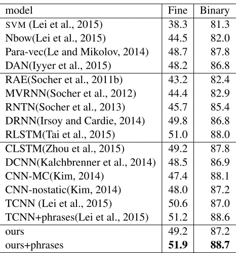
We evaluated the proposed method on three benchmark data sets: Standford Sentiment Treebank dataset (Socher et al., 2013), TREC (Text Retrieval Conference) question type classification data set (Li and Roth, 2002) and ATIS (Airline Travel Informa-tion Systems) dataset (Hemphill et al., 1990). On Standford Sentiment Treebank dataset, our model obtains 51.9% accuracy on fine-grained classifica-tion and 88.7% accuracy on binary classification. TheSVMbased method uses a large amount of

engi-neered features, and it outperforms LSTMand RNN

based methods on TREC question type classification dataset. The DLSTM outperforms other neural

net-work based methods without using engineered fea-tures. On ATIS data, DLSTM achieves 97.9% F1

score, which is better than the previous best F1 score of 95.6% using the same data settings.

2 Related Work

Deep neural networks (Bengio, 2009; Deng and Yu, 2014; Hinton et al., 2006) dominates natural lan-guage processing (Socher, 2012; Collobert et al., 2011; Gao et al., 2014). They have achieved cutting-edge performance in various tasks such as language modeling (Mikolov et al., 2010; Sundermeyer et al., 2012), machine translation (Bahdanau et al., 2014; Cho et al., 2014; Jean et al., 2015), slot fill-ing (Yao et al., 2014a; Shi et al., 2015a) and syn-tactic parsing (Wang et al., 2015; Collobert et al., 2011). For query classifications, recurrent neural networks (RNNs) and convolutional neural networks

(CNNs) have emerged as top performing

architec-tures (Zhang and Wallace, 2016; Kim, 2014; Kalch-brenner et al., 2014; Ravuri and Stolcke, 2015a).

Due to its superior ability to memorize long dis-tance dependencies, LSTMs have been applied to

extract the sentence-level continuous representation (Ravuri and Stolcke, 2015a; Tang et al., 2015; Tai et al., 2015). When theLSTMis applied to model a

sentence, memory cell from the ending word in the sentence carries the information of the whole sen-tence. The LSTM hidden vector from the ending

word is directly used as sentence feature represen-tation in (Ravuri and Stolcke, 2015a). Alternatively, a sentence is represented by the average of LSTM

hidden vectors from its words (Tang et al., 2015). Inspired from recursive neural networks (Socher et al., 2011a), LSTM is further combined with a tree

structure to model sentence representation (Tai et al., 2015).

CNNs have been originally developed for image

processing (Lecun et al., 1998). They are firstly ap-plied by Collobert et al. (2008; 2011) for natural lan-guage processing tasks using max-over-time pool-ing method to aggregate convolution layer vectors.

CNNs have also been applied to spoken language

un-derstanding (Shi et al., 2015b), information retrieval (Shen et al., 2014) and semantic parsing (Yih et al., 2015). Kalchbrenner et al. (2014) proposed to ex-tendCNNs max-over-time pooling tok-max pooling

for sentence modeling. Remarkable query classifi-cation performance on different benchmark datasets have been achieved by integratingCNNs with

differ-ent feature mapping channels and pre-trained word vectors (Zhang and Wallace, 2015; Kim, 2014). Re-cently, Mou et al. (2015) proposed to model sen-tences by tree structuredCNNs.

CNNs and LSTMs are complementary in their

modeling capabilities; CNNs are good at capturing

local invariant regularities and LSTMs are good at

modeling temporal features. The combination of

CNNs and LSTMs achieves improved performances

in speech recognition (Sainath et al., 2015) and query classification (Tang et al., 2015; Zhou et al., 2015). In these models, the basic architecture is the

LSTM that models sequence representation from

lo-cal features captured byCNNs.

non-consecutive local features. CNNs are placed on top

of these local features for query classification. Our motivation is to useLSTM replace the linear feature

mapping in convolution operation where the feature mapping is a multiplication of the word vectors with a filter matrix. So our proposed model is still CNN

based model but using DLSTM as feature mapping

for convolution operation.

Our work is closely related to tensor product basedCNNs (Lei et al., 2015) that expandCNN

fea-ture representation capacity with non-consecutiven -grams. They improve the query modeling from two aspects. Firstly, tensor products enable the non-linear feature vector interactions between adjacent words. Secondly, an exponentially decaying weight is applied to represent non-consecutiven-gram fea-tures. Instead of using tensor products as feature mapping, we propose to apply DLSTM to address

these two aspects. Nonlinear feature mapping can be achieved by the DLSTMthat equipped with

nonlin-ear activation function. The nonconsecutive feature interaction is well addressed by the memory cell and different gates in LSTM unit. In particular, the

for-get gate is able to decay the information according to the context rather than a fixed decaying weight in tensor product basedCNNs.

3 CNN Based Query Classification Using DLSTM Feature Mapping

3.1 Linear Feature Mapping in CNN

Let k-dimensional vector xt ∈ Rk be the

continu-ous feature representation of thetth word in a sen-tence. A sentence with l words is represented by

x0:l−1= [x0;x2;...;xl−1]that is a concatenation of all word vectors. The traditionalCNN(Collobert et al.,

2011; Kim, 2014) takes such sentence feature vector as input.

Different filters Mj ∈Rnd∗h are applied in

con-volution operation to map eachn-gram feature vec-torxt:t+n−1,t∈(0,l−n)to anh-dimensional feature vectorct,j.

ct,j=MTj ·xt:t+n−1+bj, (1)

wherebj is the bias in filter j.

The resulting feature vectorct,j are often passed

through non-linear element-wise transformations (e.g. the hyperbolic tangent and rectifier linear unit)

as well as pooling operations. After aggregation or reduction by different pooling operations such as the max-over-time pooling (Collobert et al., 2011; Kim, 2014) and the average pooling (Lei et al., 2015), a constant dimensional feature vector is generated for sentences with various lengths.

In traditional CNNs, the concatenated word

vec-tors are mapped linearly to feature coordinates as shown in Equation (1). Such linear feature mapping can be improved from the following two aspects, one is to extend linear mapping to nonlinear mapping. The other one is to improve the consecutive feature mapping to nonconsecutive feature mapping. For example, in the query “not a total loss”, “not loss” is the key sentiment. By using nonconsecutive fea-ture representation, the information about “not loss” could be addressed. Lei et al. (2015) extends the linear feature mapping to tensor based feature map-ping. To model the nonconsecutiven-grams, a de-caying weight is applied to control the information carryover. In this paper, we propose to replace the linear feature mapping using DLSTM that captures

the nonlinear and nonconsecutive feature interaction withinn-grams. Rather than setting a fixed decaying weight, the proposed architecture is able to control the information decaying according to the context information.

3.2 Feature Mapping Based on Deep Long Short Term Memory

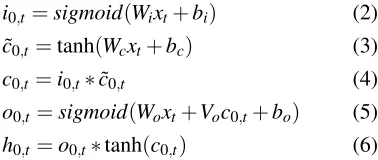
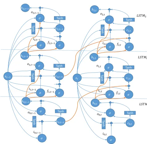
Figure 1 gives the basic architecture of a three-order nonlinear feature mapping in DLSTM. The bottom LSTM0extract the first order information from word input vectorxt. It is equipped with input gate and

output gate. The input gate automatically controls the information saving in memory cell that will be passed to higher order LSTM unit. The output gate

modifies the information from the memory cell to represent current word.

i0,t=sigmoid(Wixt+bi) (2)

˜

c0,t =tanh(Wcxt+bc) (3)

c0,t =i0,t∗c˜0,t (4)

o0,t =sigmoid(Woxt+Voc0,t+bo) (5)

h0,t =o0,t∗tanh(c0,t) (6)

𝑥𝑡−1

Tan

h

𝜎

𝑐2,𝑡−1

𝜎 Tanh

ℎ2,𝑡−1

𝜎

𝑜2,𝑡−1

Tan

h

𝜎

𝑐0,𝑡−1

𝜎 Tanh

ℎ0,𝑡−1

𝑖0,𝑡−1 𝑜0,𝑡−1

Tan

h

𝜎

𝑐1,𝑡−1

𝜎 Tanh

ℎ1,𝑡−1

𝜎

𝑜1,𝑡−1

𝑖1,𝑡−1 _𝑓

1,𝑡−1 𝑖2,𝑡−1

𝑓2,𝑡−1

𝑥𝑡

Tan

h

𝜎 𝑐2,𝑡

𝜎 Tanh

ℎ2,𝑡

𝜎

𝑜2,𝑡

Tan

h

𝜎 𝑐0,𝑡

𝜎 Tanh

ℎ0,𝑡

𝑖0,𝑡 𝑜0,𝑡

Tan

h

𝜎 𝑐1,𝑡

𝜎 Tanh

ℎ1,𝑡

𝜎

𝑜1,𝑡

𝑖1,𝑡 _𝑓

1,𝑡 𝑖2,𝑡 𝑓2,𝑡

𝐿𝑆𝑇𝑀0 𝐿𝑆𝑇𝑀1 𝐿𝑆𝑇𝑀2

Figure 1:DLSTMbased nonlinear feature mapping for bigram “xt−1xt”. ThreeLSTMunits are used to extract features from each word position. The bottomLSTM0is used for first order

feature extraction from the current word. The output from the lowerLSTMunit at current word position and the memory cell from lowerLSTMat previous word position are fed to the higher LSTMunits. Such information propagation is highlighted in the figure by bold orange lines.

stack two LSTM unitsLSTM₁ andLSTM₂ to extract

nonlinear feature representations from bigram and trigram, respectively. The LSTMj is formulated as

follows:

ij,t=sigmoid(Wixt+Uihj−1,t+bi) (7)

˜

cj,t =tanh(Wcxt+Uchj−1,t+bc) (8)

fj,t =sigmoid(Wfxt+Ufhj−1,t+bf) (9)

cj,t =ij,t∗c˜j,t∗cj−1,t−1+fj,t∗cj−1,t (10)

oj,t =sigmoid(Woxt+Uohj−1,t+Vocj,t+bo) (11)

hj,t =oj,t∗tanh(cj,t) (12)

Due to the effect from different gates that con-trols the information saving, expressing and decay-ing, LSTM1 and LSTM2 are able to model the non-consecutive interaction in n-grams. Take “not so good” as a example. LSTM0 extract the nonlinear feature mapping from word “good” as h0,2. The LSTM₁takesc_0,1(carries the information from word

“so”) andh0,2 as input. Due to the effect of forget

gate, we expect the outputh1,2 from LSTM1 to ad-dress more on word “good” rather than “so”. By further stackingLSTM2, information about the word

“not” and “good” should be emphasized by the pro-posedDLSTM.

Note the sum of the resulting outputs from these

LSTM units is used as the high order feature

rep-resentation of a n-gram ending with word xt. So

the original sequence input x0:l−1 is mapped to a sequence of feature vector z0:l−1= [z0,z1,...,zl−1], wherezj=h0,j+h1,j+h2,j.

The proposed DLSTM architecture is

character-ized by the following two features:

1. Weight Sharing: LSTM1 and LSTM2 are iden-tical LSTM units that share the same weights.

The bottomLSTM unit LSTM0 also shares the corresponding weights with other LSTM units

such as Wi, Wc and Wo. By sharing weights

among differentLSTMunits, we can effectively

reduce the risk of model over-fitting issue. At the same time,LSTMis good at capturing

tem-poral regularities. By sharing weights, the

LSTM units can learn the temporal

dependen-cies from being exposed to different order of

n-grams during the training.

2. Memory Cell Interaction: To model the nonlin-ear feature interaction inn-gram vectors, tradi-tionalLSTM unit is modified by Equation (10)

in which the memory cell stores the interaction of different order memory cells. In this way, the feature interaction inn-grams is character-ized by the memory cell interactions.

To stack the LSTM unit deeper, the depth-gated LSTM (Yao et al., 2015) and the highway network

(Srivastava et al., 2015; Zhang et al., 2015) also al-low the memory cell fal-low acrossLSTMunits at

dif-ferent depth. There are three basic differences be-tween these architectures with the proposedDLSTM.

Firstly, in their architectures,LSTMunits at different

depth are differentLSTMs that have different weight

matrices. In our model, the LSTM units in DLSTM

share weight matrices with each other. Secondly, in their proposed architecture, the memory cell is car-ried over to higherLSTM unit for facilitating model

DLSTM, the LSTM unit at higher position takes the

memory cell from lowerLSTM unit mainly for

fea-ture interaction in n-grams. Finally, an additional “depth” gate is applied in their architecture to con-trol the information flow across different layers. In our model, the input gate in higher LSTM unit

con-trols the interaction between the memory cells ex-tracted from previous word and current word.

3.3 The Architecture

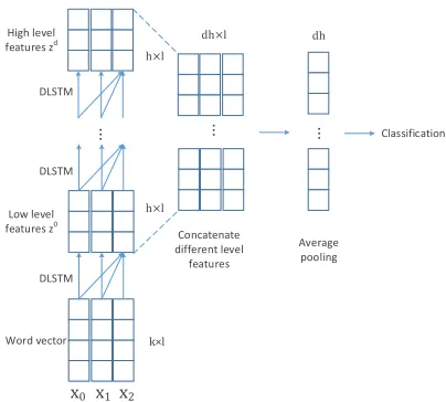
Figure 3 gives the whole architecture of the pro-posed query classification system. A DLSTMlayer

first maps the input sequence to a sequence of high order nonlinear feature representationsz0_{. Instead of} being directly used for query classification, the fea-ture representationz0_{is further processed by a stack} ofDLSTM layers illustrated in previous section. In

such stacked DLSTMlayers, the outputzi of theith DLSTMlayer, is used as the input for thei+1thDL -STMlayer parameterized by a different set of weight

matrices. As shown in Figure 3, the resulting fea-ture representations z0_,z1_,...,zd _{of all these layers}

are concatenated. Finally, an average pooling is ap-plied to reduce the sentence feature representation to a fixed dimensional vector that is further fed to a softmax function to obtain the prediction output.

3.4 Learning and Regularization

In the classification layer, the prediction output is obtained by the following softmax function.

so ftmax(y)j= exp(yj)

∑ii==1mexp(yi), (13)

where y is a m-dimensional vector. The model is trained by minimizing cross-entropy on the given training data set. To avoid overfitting during train-ing, L2 regularization and dropout (Hinton et al., 2012) are used. TheL2 regularization is applied to constrain all weight matrices using the same regu-larization weight. The dropout is only applied to the output of eachDLSTMlayer.

In the training, the model weights are updated using mini-batch stochastic gradient descent (SGD).

We adapt a per-feature learning rate control method (AdaGrad) (Duchi et al., 2011) to dynamically tune the learning rate as follows:

αt,i= q α

∑tj=1g2j,i+ε

, (14)

Word vector Low level features z0

High level features zd

...

DLSTM DLSTM DLSTM

x0 x1 x2

...

Concatenate different level

features

...

Classification

Average pooling

k×l h×l h×l

dh×l dh

Figure 2:CNNbased query classification usingDLSTMfeature

mapping. The input sequence is represented by ak×lmatrix where columntis the word vector for thetth word in the se-quence. The word vectors are mapped by a stack of DLSTM

layers to multi-level feature representationsz0_,...,zd_{. As} illus-trated in Figure 1, each level feature representation is the sum of outputs from differentLSTMunits. The multi-level features

are concatenated and reduced to adh-dimensional vector where dis the number ofDLSTMlayers,his the output size of each LSTMunit. A classification layer gives the prediction output.

whereαt,iis the learning rate for weightiat epocht.

∑t_j=1gj,i sums all the historical gradients of weight

i. A small positiveεis applied to make the AdaGrad robust.εis usually set to 1e−5.

4 Experiments

4.1 Datasets

sentences. The binary classification task in this dataset has 6920 sentences for training, 872 sen-tences for developing and 1821 sensen-tences for test-ing. There are in total 17835 unique running words for fine-grained dataset and 16185 for binary version dataset.

For query intent detection, ATIS (airline travel in-formation system) dataset (Hemphill et al., 1990; Yao et al., 2014b) is used. This dataset is mainly about the air travel domain with 26 different intents such as “flight”, “groundservice” and “city”. There

are 893 utterances for testing (ATIS-III, Nov93 and Dec94), and 4978 utterances for training (rest of ATIS-III and ATIS-II). There are 899 unique run-ning words and 22 intents in the trairun-ning data.

The question type classification task is to clas-sify a question into a specific type, which is a very important step in question answering system. In TREC (Text Retrieval Conference) data (Li and Roth, 2002), all the questions are divided into 6 categories, including “human”, “entity”, “location”, “description”, “abbreviation” and “numeric”. The dataset in total has 5952 questions, 5452 of them for training, the rest for testing. The vocabulary size of TREC dataset is 9592.

Following previous work (Iyyer et al., 2015; Tai et al., 2015; Lei et al., 2015), we used word vectors pre-trained on large unannotated corpora to achieve better generalization capability. In this paper, we used a publicly available 300 dimensional GloVe word vectors that are trained using Common Crawl with 840B tokens and 2.2M vocabulary size.

4.2 Settings

We implemented our model based on Theano library (Bastien et al., 2012). All our models are trained on Nvidia Tesla K40m.

We performed extensive hyperparameter selection based on Stanford Sentiment Treebank Binary ver-sion of validation data. The selected hyperparame-ters were directly used for all datasets. To investi-gate the robustness of the proposed method, we ran each configuration 10 times using different random initialization (random seed ranges from 1 to 10).

For final models, we set the initial learning rate to 0.1,L2 regularization weight to 1e−5, the dropout probability to 0.5 and mini-batch size to 64. We use hidden layer size 256 for all the models described in

model Fine Binary

SVM(Lei et al., 2015) 38.3 81.3

Nbow(Lei et al., 2015) 44.5 82.0 Para-vec(Le and Mikolov, 2014) 48.7 87.8 DAN(Iyyer et al., 2015) 48.2 86.8 RAE(Socher et al., 2011b) 43.2 82.4 MVRNN(Socher et al., 2012) 44.4 82.9 RNTN(Socher et al., 2013) 45.7 85.4 DRNN(Irsoy and Cardie, 2014) 49.8 86.8 RLSTM(Tai et al., 2015) 51.0 88.0 CLSTM(Zhou et al., 2015) 49.2 87.8 DCNN(Kalchbrenner et al., 2014) 48.5 86.9

CNN-MC(Kim, 2014) 47.4 88.1

CNN-nostatic(Kim, 2014) 48.0 87.2 TCNN (Lei et al., 2015) 50.6 87.0 TCNN+phrases(Lei et al., 2015) 51.2 88.6

ours 49.2 87.2

ours+phrases 51.9 88.7

Table 1:Standford Sentiment Treebank Classification accuracy results. “Fine” denotes the accuracy on the fine-grained dataset with 5 labels. “Binary” denotes binary classification results.

the experiments. The number of the DLSTMlayers

and the number of the LSTM units in each DLSTM

are both set to 3. So basically there are 9LSTMunits

are used for each word position.

For all models, we set maximum iteration num-ber 100 to terminate the training process. For sen-timent classification task, during the training, the model with the best classification accuracy on val-idation data was used as final model for testing. For question type classification and query intent detec-tion, there wasn’t validation data. So we simply use the model trained at the 100th iteration as the final model for testing.

4.3 Results on Stanford Sentiment Treebank

model Acc

discriminative(Tur et al., 2010) 95.5

SVM(Shi et al., 2015b) 95.6

joint-RNN(Shi et al., 2015b) 95.2

ours 97.9

Table 2:ATIS intent classification accuracy comparison of dif-ferent models.

There are four blocks in the table. The bottom block gives the results from our model. The third blocks are methods related to CNNs. The second

block shows the results from recursive neural net-work based approaches. The other baseline methods are listed in the top block.

The top block shows that the traditional methods such as SVM using ngram features and neural

net-work using bag-of-words features (Nbow) perform much worse than Para-vec and DAN using word vectors that are pre-trained on large amount of un-labeled data. Para-vec builds a logistic regression on top of paragraph vectors. DANis a deep neural network takes the average of word vectors as input.

In addition to pre-trained word vectors, syntac-tic compositional information can be used to im-prove the sentiment classification accuracy. RAEis a tree structured Antoencoder model based on pre-trained word vectors from Wikipedia.MVRNN fur-ther improves the recursive neural network by as-signing each node with a matrix to learn the meaning change of neighboring words and phrases. To ad-dress large amount of different vectors and matrices involved inMVRNN, RNTN proposed to use one single tensor based function to model all nodes. By making the tree-structured recursive neural networks deeper, significant improvement has been achieved by DRNN. According to our knowledge, the best compositional information based model is achieved

by RLSTM that combines LSTM unit with

tree-structure.

By comparing the classification accuracy between second blocks and third blocks, we see that CNN

based models in general perform better than recur-sive neural network based methods. Another advan-tage ofCNN based methods is that they can be

gen-eralized to any language without dependency over compositional information. DCNN uses a dynamic

k-max pooling operator function inCNN. To explore

the task specific word vectors and the general word vectors pre-trained on large News dataset, CNN-MCequipsCNNwith two feature mapping channels.

CNN-nostaticgives the results by only making use

of general word vectors. The best published classi-fication results are achieved byTCNNthat is tensor basedCNN.

In this paper, the proposed method is closely re-lated toTCNN. Instead of using tensor products to

replace linear convolution operation, our method ex-ploits the nonlinear feature mapping through DL -STM. Rather than setting specific decaying weight

to model non-consecutiven-gram features in tensor based CNN, the different gates automatically adjust

the information storing, removing and outputting ac-cording to context.

Following the work of TCNN, to leverage the phrases level annotation in Standford Sentiment Treebank, all phrases and their corresponding labels are added to training data as additional sequences. The bottom line of Table 1 shows that our models achieved the state-of-the-art performance on senti-ment classification task.

For the best settings described above, we ran each model 10 times with different random initialization. The average and standard deviation for fine-grained classification are 50.7% and 1.04%, for binary clas-sification 88% and 0.41%. Comparing withTCNN, our model is more sensitive to the parameter random initialization. In the future, some efforts should be used to analyze and address this issue.

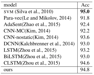
model Acc

SVM(Silva et al., 2010) 95.0

Para-vec(Le and Mikolov, 2014) 91.8 AdaSent(Zhao et al., 2015) 92.4

CNN-MC(Kim, 2014) 92.2

CNN-nostatic(Kim, 2014) 93.6 DCNN(Kalchbrenner et al., 2014) 93.0 LSTM(Zhou et al., 2015) 93.2 BiLSTM(Zhou et al., 2015) 93.0 CLSTM(Zhou et al., 2015) 94.6

ours 94.8

Table 3:TREC Question type Classification accuracy compar-ison of different models.

4.4 Results on ATIS

ATIS dataset is widely used to test spoken language understanding system. As shown in Table 2, SVM

usingn-grams performs better than simpleRNNand CNN based approach. joint-RNNis a query

classi-fication and slot filling joint training model where

CNNis applied on top of slot taggingRNNfor query

ad--2 -1 0 1 2

not so good

Negative Prediction

-2 -1 0 1 2

a successful failure

Negative Prediction

-2 -1 0 1 2

hardly to be bad

Postive Prediction

-2 -1 0 1 2

a waste of good performance

Negative Prediction (groundtruth:Negative)

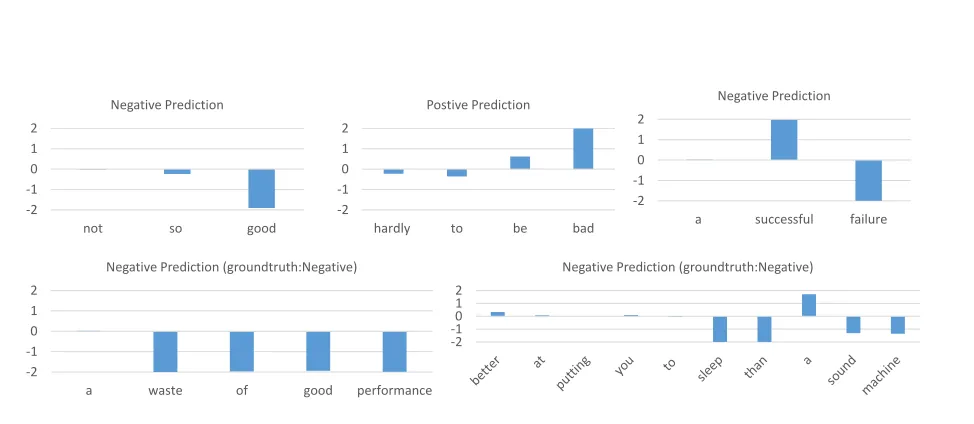
-2 -10 1 2

Negative Prediction (groundtruth:Negative)

Figure 4: Example predictions given by our model trained on Stanford Sentiment Treebank fine-grained data. The expected sentiment score of each word is plotted in the figure. The score range from−2 to 2, where a score−2 means very “negative”, 0 stands for “neutral” and 2 means “very positive”.

84.5 85 85.5 86 86.5 87 87.5 88 88.5 89

85 85.5 86 86.5 87 87.5 88 88.5 89 89.5

Tes

t

ac

cu

rac

y

Validation accuracy

depth 3 depth 2 depth 1

Figure 3: Stanford Sentiment Treebank Binary Classification accuracy comparison among models using the same parameter configuration except the number of DLSTM layers. For each number ofDLSTMlayers, 10 models are run independently us-ing different random initialization. Horizontal axis gives the validation accuracy. Vertical axis shows the test accuracy.

vantage of word vectors trained on large amount of unlabeled data. Based on pre-trained word vectors, our models obtain more than 2% absolute classifica-tion accuracy improvement over the published best model.

In ATIS data, about 70% of queries is categorized to “flight” intent. Recent work using RNN for

ut-terance classification (Ravuri and Stolcke, 2015b;

Ravuri and Stolcke, 2015a) simplifies it to a “flight” VS “others” binary classification task. In their paper, using word basedLSTM, they achieve 97.55%

clas-sification accuracy. By using extra name entity fea-tures, word based gatedRNNobtains 98.42%

classi-fication accuracy.

4.5 Results on TREC Question Type Classification

Table 3 gives the TREC question type classification accuracy of our models with other baseline mod-els. Different from the sentiment classification task, the shallow models using diverse engineered feature performs better thanCNN andLSTMbased models.

Previous best classification results on TREC data is achieved by SVM using unigrams, bigrams,

wh-word, head wh-word, POS tags, hypernyms, WordNet synsets and a bunch of hand-coded rules.

AdaSent is a self adaptive hierarchical sentence

model based on gating networks with level pooling. As shown in Table 3,CNNandLSTMachieve similar

performances on question type classification. Re-cently CLSTM achieves substantial improvement over previous neural network based methods. In

CLSTM, CNN is used to extract high level phrase

fed intoLSTMto model whole sequence

representa-tion. Different withCLSTMthat is anLSTMbased

sequence model with CNN for local feature

extrac-tion, our model is CNN based model using DLSTM

for non-linear feature mapping. Our model outper-forms previous neural network based models with-out relying on task specific feature engineering.

4.6 Deep Architecture

One critical hyperparameter in the proposed method is the number of DLSTM layers. On sentiment

bi-nary classification task, we run our model 10 times by keeping all the hyperparameters the same except the number ofDLSTMlayers using different random

initialization. As observed from Figure 3, the bet-ter performance is achieved by deeper architecture. Our model achieves the best classification result by stacking 3 DLSTM layers that actually leverages 9

differentLSTMunits to extract the nonlinear feature

fromn-grams.

4.7 Examples

Figure 4 demonstrates some examples and their sen-timents predicted by our model trained on fine-grained classification data. In order to see how the nonlinear feature mapping captures the sentiment at each word position in the query, we follow the strategy used in (Lei et al., 2015) where the soft-max function is directly applied on the concatenated feature mapping without passing through the aver-age pooling layer. So the sentiment distribution pt

at tth word is computed as pt =WT[zt0,z1t,...,zdt].

The expected value over the probability distribution ∑2s=−2s.pt is used as the sentiment score that is

plot-ted in Figure 4. In the figure, the sentiment score ranges from −2 to 2, where−2 means very nega-tive, 2 mean very positive and 0 means neutral.

Five examples are illustrated in the figure where the first row gives the synthetic examples to show that our model is able to model the nonconsecutive interaction withinn-grams. For example, in query “hardly to be bad”, even though word “hardly” is not directly modifying word “bad”, our model still be able to capture such sentiment changes.

The second row of the figure shows the examples from fine-grained classification testing data. Both the example show that our model to some degree can capture sentiment of the satire. Especially the

last example, our model actually gives negative pre-diction, even no word in the query really means neg-ative.

5 Conclusions

We have proposed a deep long-short-term-memory (DLSTM) nonlinear nonconsecutive feature mapping

architecture to replace traditional linear mapping in the convolutional neural network based query clas-sification. EachLSTMunit in the DLSTMis

respon-sible for capturing different order feature represen-tation from word segments. The bottomLSTM unit

equipped with input gate and output gate, extracts the nonlinear feature from unigram. The higher

LSTM unit in the DLSTM takes the outputs from

lowerLSTM units as input. In such way, the higher LSTM unit is able to capture nonlinear feature

rep-resentation from higher ordern-grams. The sum of differentLSTMunits is used as the output of theDL -STMlayer. TheDLSTMoutput rather than being

di-rectly used as input to convolutional neural network for query classification, is passed through a stacked

DLSTM layers. The query is finally represented by

the concatenation of the outputs from the stacked

DLSTMlayers.

We evaluated the proposed models on three benchmark datasets–Stanford Sentiment Treebank dataset, TREC dataset and ATIS dataset. On both sentiment classification dataset and ATIS dataset, our model achieved the state-of-the-art performance. On TREC question type classification, SVM based

model using extra engineered features still per-formed better than our model. But we noticed that the proposed method outperformed all the other neu-ral network based approaches.

References

Dzmitry Bahdanau, Kyunghyun Cho, and Yoshua Ben-gio. 2014. Neural machine translation by jointly learning to align and translate. CoRR.

Fr´ed´eric Bastien, Pascal Lamblin, Razvan Pascanu, James Bergstra, Ian J. Goodfellow, Arnaud Berg-eron, Nicolas Bouchard, and Yoshua Bengio. 2012. Theano: new features and speed improvements. In

Deep Learning and Unsupervised Feature Learning

NIPS 2012 Workshop.

Yoshua Bengio. 2009. Learning deep architectures for

Kyunghyun Cho, Bart van Merrienboer, Caglar Gulcehre, Fethi Bougares, Holger Schwenk, and Yoshua Ben-gio. 2014. Learning phrase representations using rnn encoder-decoder for statistical machine translation. In

EMNLP.

Ronan Collobert and Jason Weston. 2008. A unified ar-chitecture for natural language processing: Deep neu-ral networks with multitask learning. In The Pro-ceedings of the International Conference on Machine

Learning, pages 160–167.

Ronan Collobert, Jason Weston, L´eon Bottou, Michael Karlen, Koray Kavukcuoglu, and Pavel Kuksa. 2011. Natural language processing (almost) from scratch.

Journal of Machine Learning Research, 12:2493–

2537.

Li Deng and Dong Yu. 2014. Deep learning: Meth-ods and applications. Found. Trends Signal Process., 7:197–387.

John Duchi, Elad Hazan, and Yoram Singer. 2011. Adaptive subgradient methods for online learning and stochastic optimization. Journal of Machine Learning

Research, 12:2121–2159.

Jianfeng Gao, Xiaodong He, Wen-tau Yih, and Li Deng. 2014. Learning continuous phrase representations for translation modeling. In Proceedings of ACL, pages 699–709.

Alan Graves, Abdel-rahman Mohamed, and Geoffrey Hinton. 2013. Speech recognition with deep recurrent neural networks. In The proceedings of IEEE Inter-national Conference on Acoustics, Speech and Signal

Processing, pages 6645–6649.

Charles T. Hemphill, John J. Godfrey, and George R. Doddington. 1990. The atis spoken language systems pilot corpus. InThe Proceedings of the Workshop on

Speech and Natural Language, pages 96–101.

Geoffrey E. Hinton, Simon Osindero, and Yee-Whye Teh. 2006. A fast learning algorithm for deep belief nets.

Neural Comput., 18(7):1527–1554.

Geoffrey E. Hinton, Nitish Srivastava, Alex Krizhevsky, Ilya Sutskever, and Ruslan R. Salakhutdinov. 2012. Improving neural networks by preventing co-adaptation of feature detectors. CoRR.

Sepp Hochreiter and J¨urgen Schmidhuber. 1997. Long short-term memory. Neural Comput., 9(8):1735– 1780.

Ozan Irsoy and Claire Cardie. 2014. Deep recursive neu-ral networks for compositionality in language. In

Pro-ceedings of NIPS, pages 2096–2104.

Mohit Iyyer, Varun Manjunatha, Jordan L. Boyd-Graber, and Hal Daum´e III. 2015. Deep unordered composi-tion rivals syntactic methods for text classificacomposi-tion. In

Proceedings of ACL, pages 1681–1691.

S´ebastien Jean, Kyunghyun Cho, Roland Memisevic, and Yoshua Bengio. 2015. On using very large target vo-cabulary for neural machine translation. In

Proceed-ings of ACL, pages 1–10.

Nal Kalchbrenner, Edward Grefenstette, and Phil Blun-som. 2014. A convolutional neural network for mod-elling sentences. InProceedings of ACL, June. Yoon Kim. 2014. Convolutional neural networks for

sen-tence classification. InProceedings of the 2014 Con-ference on Empirical Methods in Natural Language

Processing (EMNLP), pages 1746–1751, October.

Quoc V. Le and Tomas Mikolov. 2014. Distributed rep-resentations of sentences and documents. In

Proceed-ings of ICML, pages 1188–1196.

Y. Lecun, L. Bottou, Y. Bengio, and P. Haffner. 1998. Gradient-based learning applied to document recog-nition. Proceedings of the IEEE, 86(11):2278–2324, Nov.

Tao Lei, Regina Barzilay, and Tommi S. Jaakkola. 2015. Molding cnns for text: non-linear, non-consecutive convolutions. InProceedings of the 2015 Conference on Empirical Methods in Natural Language Process-ing, pages 1565–1575.

Xin Li and Dan Roth. 2002. Learning question classi-fiers. In Proceedings of the 19th International

Con-ference on Computational Linguistics, COLING ’02,

pages 1–7.

Tomas Mikolov, Martin Karafi´at, Lukas Burget, Jan Cer-nock´y, and Sanjeev Khudanpur. 2010. Recurrent neu-ral network based language model. InThe

Proceed-ings of Interspeech, pages 1045–1048.

Lili Mou, Hao Peng, Ge Li, Yan Xu, Lu Zhang, and Zhi Jin. 2015. Tree-based convolution: A new neural ar-chitecture for sentence modeling. CoRR.

Suman Ravuri and Andreas Stolcke. 2015a. A compar-ative study of neural network models for lexical intent classification. InThe Proceedings of IEEE Automatic

Speech Recogntion and Understanding Workshop.

Suman Ravuri and Andreas Stolcke. 2015b. Recurrent neural network and lstm models for lexical utterance classification. InProceedings of Interspeech.

Tara N. Sainath, Oriol Vinyals, Andrew W. Senior, and Hasim Sak. 2015. Convolutional, long short-term memory, fully connected deep neural networks. In

Proceedings of ICASSP, pages 4580–4584.

Yelong Shen, Xiaodong he, Jianfeng Gao, Li Deng, and Gregoire Mesnil. 2014. Learning semantic represen-tations using convolutional neural networks for web search. InProceedings of WWW. WWW 2014, April. Yangyang Shi, Kaisheng Yao, Hu Chen, Yi-Cheng Pan,

Yangyang Shi, Kaisheng Yao, Hu Chen, Yi-Cheng Pan, Mei-Yuh Hwang, and Baolin Peng. 2015b. Contextual spoken language understanding using recurrent neural networks. In The Proceedings of International

Con-ference on Acoustics, Speech and Signal Processing.

J. Silva, L. Coheur, A. C. Mendes, and Andreas Wichert. 2010. From symbolic to sub-symbolic information in question classification. Artificial Intelligence Review. Richard Socher, Cliff C. Lin, Andrew Y. Ng, and

Christo-pher D. Manning. 2011a. Parsing Natural Scenes and Natural Language with Recursive Neural Networks.

InProceedings of ICML.

Richard Socher, Jeffrey Pennington, Eric H. Huang, An-drew Y. Ng, and Christopher D. Manning. 2011b. Semi-supervised recursive autoencoders for predicting sentiment distributions. In Proceedings of EMNLP, pages 151–161.

Richard Socher, Brody Huval, Christopher D. Manning, and Andrew Y. Ng. 2012. Semantic Compositional-ity Through Recursive Matrix-Vector Spaces. In Pro-ceedings of the Conference on Empirical Methods in

Natural Language Processing.

Richard Socher, Alex Perelygin, Jean Wu, Jason Chuang, Christopher D. Manning, Andrew Ng, and Christopher Potts. 2013. Recursive Deep Models for Semantic Compositionality Over a Sentiment Treebank. In Pro-ceedings of the Conference on Empirical Methods in

Natural Language Processing, pages 1631–1642.

Richard Socher. 2012. New directions in deep learning: Structured models, tasks, and datasets. Neural Infor-mation Processing Systems (NIPS) Workshop on Deep

Learning and Unsupervised Feature Learning.

Rupesh Kumar Srivastava, Klaus Greff, and J¨urgen Schmidhuber. 2015. Highway networks. CoRR, abs/1505.00387.

Martin Sundermeyer, Ralf Schl¨uter, and Hermann Ney. 2012. LSTM neural networks for language modeling.

InINTERSPEECH, pages 194–197.

Ilya Sutskever, Oriol Vinyals, and Quoc V. Le. 2014. Se-quence to seSe-quence learning with neural networks. In

Advances in Neural Information Processing Systems,

pages 3104–3112.

Kai Sheng Tai, Richard Socher, and Christopher D. Man-ning. 2015. Improved semantic representations from tree-structured long short-term memory networks. In

Proceedings of ACL, pages 1556–1566. Association

for Computational Linguistics, July.

Duyu Tang, Bing Qin, and Ting Liu. 2015. Document modeling with gated recurrent neural network for sen-timent classification. InProceedings of the 2015 Con-ference on Empirical Methods in Natural Language

Processing, pages 1422–1432.

G. Tur, D. Hakkani-Tur, and L. Heck. 2010. What is left to be understood in atis? In Spoken Language

Technology Workshop (SLT), 2010 IEEE, pages 19–24.

Peilu Wang, Yao Qian, Frank K. Soong, Lei He, and Hai Zhao. 2015. A unified tagging solution: Bidi-rectional LSTM recurrent neural network with word embedding. CoRR.

Kaisheng Yao, Baolin Peng, Yu Zhang, Dong Yu, Geof-frey Zweig, and Yangyang Shi. 2014a. Spoken lan-guage understanding using long short-term memory neural networks. InThe Proceedings of IEEE

work-shop on Spoken Language Technology, pages 189–

194.

Kaisheng Yao, Baolin Peng, Yu Zhang, Dong Yu, Geof-frey Zweig, and Yangyang Shi. 2014b. Spoken lan-guage understanding using long short-term memory neural networks. InThe Proceedings of IEEE

work-shop on Spoken Language Technology, pages 189–

194.

Kaisheng Yao, Trevor Cohn, Katerina Vylomova, Kevin Duh, and Chris Dyer. 2015. Depth-gated LSTM.

CoRR.

Wen-tau Yih, Ming-Wei Chang, Xiaodong He, and Jian-feng Gao. 2015. Semantic parsing via staged query graph generation: Question answering with knowl-edge base. InProceedings of ACL, pages 1321–1331. Ye Zhang and Byron Wallace. 2015. A sensitivity

analy-sis of (and practitioners’ guide to) convolutional neural networks for sentence classification. CoRR.

Ye Zhang and Byron Wallace. 2016. A sensitivity analy-sis of (and practitioners’ guide to) convolutional neural networks for sentence classification. InCoRR. Yu Zhang, Guoguo Chen, Dong Yu, Kaisheng Yao,

San-jeev Khudanpur, and James Glass. 2015. Highway long short-term memory rnns for distant speech recog-nition.CoRR.

Han Zhao, Zhengdong Lu, and Pascal Poupart. 2015. Self-adaptive hierarchical sentence model. CoRR. Chunting Zhou, Chonglin Sun, Zhiyuan Liu, and Francis