Pathological Motion Detection for Robust Missing Data Treatment

Volume 2008, Article ID 542436,16pages doi:10.1155/2008/542436

Research Article

Pathological Motion Detection for Robust

Missing Data Treatment

David Corrigan, Naomi Harte, and Anil Kokaram

Department of Electronic and Electrical Engineering, Trinity College Dublin, Dublin 2, Ireland

Correspondence should be addressed to David Corrigan,[email protected]

Received 31 August 2007; Accepted 3 April 2008

Recommended by Peter Schallauer

This paper presents a new missing data detection algorithm that is robust to pathological motion (PM). PM causes clean image data to be misdiagnosed as missing data, resulting in damage to the image during restoration. The proposed algorithm uses a probabilistic framework to jointly detect PM and missing data. It builds on an existing technique of using five frames for detection instead of the standard three frames. This allows the temporally impulsive intensity profile of blotches to be distinguished from the quasiperiodic profile of PM. Another diagnostic for PM is defined on the motion fields of the five-frame window. This follows the observation that PM results in motion fields which are not smooth. A ground truth comparison with standard missing data detectors shows that the proposed algorithm dramatically reduces the number of falsely detected missing data regions. It is also shown to reduce image damage during missing data treatment.

Copyright © 2008 David Corrigan et al. This is an open access article distributed under the Creative Commons Attribution License, which permits unrestricted use, distribution, and reproduction in any medium, provided the original work is properly cited.

1. INTRODUCTION

Missing data treatment is an important process in the digital restoration of archived media. It is concerned with the re-moval of visible impairments, known as blotches, commonly present in archived sequences. Also referred to as “dirt and sparkle,” blotches are caused by either adherence of dirt to the surface of the film emulsion, or by abrasion of the emulsion. Consequently, blotches manifest as typically small dark or bright regions in the digital sequence which obscures the true image data. Missing data treatment (MDT) algorithms attempt to detect these blotches and to somehow recover the true image data.

Most blotch detection algorithms are derived from the assumption that if a blotch is present at a particular location in a frame, then no blotches are present at the same point in neighbouring frames. Blotches are therefore considered to be a temporally impulsive event due to the change in intensity from the true intensity to the blotch intensity at a particular pixel. Detection of blotches can be performed by searching for sites where temporal discontinuities exist between the current frame and the previous and next frames. Consequently, missing data detectors employ a

three-frame window and detect discontinuities by measuring the displaced frame difference (DFD) between the appropriate frames. Examples of detectors using a three-frame window include the deterministic spike detection index (SDI) [1,2] and rank order distance (ROD) [3,4] detectors, which apply deterministic thresholds to the DFDs to detect discontinu-ities, and the probabilistic Morris [2,5] and blotch MRF [6] algorithms, which allow for the inclusion of prior knowledge of the result into the decision. Other detectors [1,7] propose methods for the estimation of a nonbinary blotch confidence index.

(a) (b)

(c) (d)

(e) (f)

Figure1: Left: three consecutive frames of a sequence where the motion of the propellor blades is PM (repetitive occlusion); right: the images after MDT using [10]. The arrows indicate the removal of the blades due to the blades being misdiagnosed a blotch.

extensive taxonomies of PM are presented in [8, 9]. PM affects the robustness of blotch detectors as it can also cause temporal discontinuities.

In this paper, a new missing data detection algorithm is presented. The algorithm is made more robust by preventing PM regions being detected as blotches, thereby preventing damage to image data during restoration of dirty sequences. A five-frame window is used instead of the standard three frames. This allows blotches to be distinguished from long term forms of PM, since blotches have a temporally impul-sive intensity profile and PM often causes the intensity to vary in a periodic manner (seeFigure 2). The next section introduces a review of the existing approaches to improve the robustness of blotch detection to PM and outlines the motivation for the new algorithm. The algorithm is then outlined in Sections3and4.Section 5presents an evaluation of the algorithm, including the results of an experimental comparison of the new detector with existing blotch detec-tors on two ground truth sequences. The paper concludes with a discussion of the algorithm, outlining areas for future development.

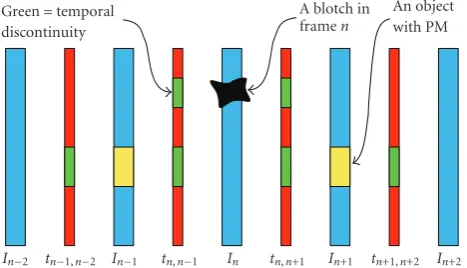
Green=temporal discontinuity

A blotch in framen

An object with PM

In−2 tn−1,n−2 In−1 tn,n−1 In tn,n+1 In+1 tn+1,n+2 In+2

Figure2: This figure illustrates the arrangement of the five frames window for blotch detection (in blue). The window is centred on framen(In) which is the frame on which blotch detection is to be

performed. Between the five frames, four temporal discontinuity fields (t∗,∗) (in red) can be estimated between pairs of consecutive

frames. In this diagram a blotch is present on frame nand the yellow object is occluded in every second frame (an example of PM). Due to the pattern of occlusion it is impossible to distinguish between the blotch and the object when detecting blotches based on temporal discontinuities over a three-frame window. By extending the window it is possible to perform a correct diagnosis.

2. REVIEW OF PM DETECTION ALGORITHMS

Previous approaches for dealing with PM have largely fallen into three categories. The first strategy is to recognise that PM is associated with the motion of foreground objects. Therefore, by performing a foreground/background segmen-tation, likely PM regions can be associated with the estimated foreground and missing data detection can be made more conservative in these regions [6]. The second uses the colour statistics of blotches and PM regions (specifically motion blur) to distinguish between them [11]. This is possible as blotches typically manifest as regions of dark or bright intensity while motion blur is the apparent smearing of a foreground object over a background.

The final approach is to extend the temporal window for blotch detection from three to five frames. This approach was first adopted by van Roosmalen in [12], in which the ROD detector was modified to operate on a five-frame window. Another more elaborate algorithm adopting this approach is outlined by Bornard in [9]. In the Bornard algorithm a probabilistic framework is used to estimate the four binary temporal discontinuity fields over a five-frame window (see

Figure 2). This is followed by a deterministic interpretation step to perform the classification. Missing data is classified if temporal discontinuities only exist at a site in the two central discontinuity fields. Sites at which discontinuities also exist in the two outer fields are classified as PM.

for prior knowledge of the blotch and PM masks as well as the temporal discontinuity fields (TDFs) to be included in the framework. The second novelty to algorithm is the addition of a further decision criterion for PM based on the smoothness of the motion fields. This follows from the observation that PM causes the local smoothness assumption of a motion field to be violated. The vector field divergence is used as the smoothness measure in the proposed algorithm.

Section 3outlines the blotch and PM detection model employed in the algorithm and how this relates to the tempo-ral discontinuity and motion field smoothness information.

Section 4describes how the two detection criteria are inte-grated into the probabilistic framework and subsequently introduces the new algorithm.

3. ALGORITHM OVERVIEW

The goal of the algorithm is to segment the current frame into regions of PM, missing data, and uncorrupted sites. To achieve this, a label field,l(x), is defined as follows:

l(x)= ⎧ ⎪ ⎪ ⎨ ⎪ ⎪ ⎩

0 no missing data or pathological motion, 1 missing data,

2 pathological motion.

(1)

Every pixel in the image is assigned one of the three labels. Like the Bornard algorithm, a pixel cannot be both a missing data site and a PM site. Although there is no reason why a blotch could not occur in a PM region, it would not be possible to reliably detect a blotch using a purely temporal discontinuity-based detector. Furthermore, a PM detection implies that the data at any blotch cannot be interpolated temporally. Consequently, interpolation must be performed using spatial rather than temporal information.

3.1. Temporal discontinuity-based detection

Like the Bornard algorithm, the DFD between a pair of neighbouring frames is used as the measure of temporal discontinuity. A temporal discontinuity is said to exist at a given site if the absolute value of the DFD at the site is sufficiently large. In the five frame window, there are four pairs of neighbouring frames where the frames are denoted byIn−2(x),In−1(x),In(x),In+1(x), andIn+2(x). A DFD can be measured between each pair with a binary temporal discon-tinuity field associated with each DFD. Consequently, four DFDs (Δn−2(x),Δn−1(x),Δn+1(x), and Δn+2(x)) and TDFs (t(x)=[tn−2(x),tn−1(x),tn+1(x),tn+2(x)]) are estimated over

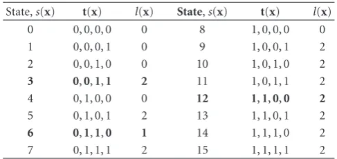
the five-frame window. In the proposed algorithm, all con-figurations of temporal discontinuity are considered. There are sixteen possible configurations of the four TDFs and a state fields(x) is defined which describes the configuration of a site. Each configuration is directly mapped to a value of l(x) (Table 1).

Missing data regions are characterised by an impulsive temporal intensity profile. Therefore, if a blotch exists in frame n, the absolute values of the DFDs between both frames n and n − 1(Δn−1(x)) and frames n and n + 1(Δn+1(x)) will be large but the other two DFDs will have

Table1: The temporal discontinuity model for the framework.

State,s(x) t(x) l(x) State,s(x) t(x) l(x)

0 0, 0, 0, 0 0 8 1, 0, 0, 0 0

1 0, 0, 0, 1 0 9 1, 0, 0, 1 2

2 0, 0, 1, 0 0 10 1, 0, 1, 0 2

3 0,0,1,1 2 11 1, 0, 1, 1 2

4 0, 1, 0, 0 0 12 1,1,0,0 2

5 0, 1, 0, 1 2 13 1, 1, 0, 1 2

6 0,1,1,0 1 14 1, 1, 1, 0 2

7 0, 1, 1, 1 2 15 1, 1, 1, 1 2

Table2: The divergence state model for the probabilistic frame-work.

Divergence state,v(x) l(x) s(x)

0 0,1 0, 1, 2, 4, 6, 8

1 2 3, 5, 7, 9, 10, 11, 12, 13, 14, 15

small values (see Figure 2). This results in a predictable temporal discontinuity profile described by s(x) = 6 in

Table 1. On the other hand, the quasiperiodic profile of long-term PM will result in high absolute values in more than two DFDs. Consequently, any temporal discontinuity configuration with two or more temporal discontinuities present, apart from the missing data case, is considered to be associated with PM (Table 1). In the table, states 3 and 12 can correspond to missing data in the neighbouring frames. It is considered here as PM as it is not caused by missing data in the current frame.

In the Bornard algorithm, all candidate blotch sites are found (i.e., wheretn−1(x)= tn+1(x)= 1) before each can-didate is classified as either being a blotch site or PM site. This is performed based on the frequency of discontinuity in tn−2(x) andtn+2(x) in the neighbourhood of the candidate.

Effectively, this means that not every configuration of tem-poral discontinuity is detected, distinguishing the Bornard algorithm from the proposed algorithm.

3.2. Motion field smoothness based detection

The second feature used to detect PM is the smoothness of the motion field. The vector field divergence is used as the basis of the smoothness measure. By estimating the divergences of all the motion fields in the five-frame window, a smoothness energy term, Ediv(x), can be defined which describes the smoothness of the motion fields. This measure of divergence will be large in the presence of long-term PM and low in other cases. The divergence measure is associated with a binary fieldv(x), where a value of 0 corresponds to a low divergence measure (i.e., when motion is not patho-logical) and a value of 1 corresponds to a high divergence measure (i.e., for PM). This relationship is described in

Table 2.

given value ofsorv, the value oflis directly defined through Tables1and2.

4. PROBABILISTIC FRAMEWORK

The framework derives an estimate ofs(x) from the posterior P(s(x) | Δn(x),Ediv(x)). For convenience of notation, the

four DFDs have been grouped into a vector-valued function

ΔnwhereΔn(x)=[Δn−2(x),Δn−1(x),Δn+1(x),Δn+2(x)]. The posterior is factorised in a Bayesian fashion as fol-lows:

Ps|Δn,Ediv

∝ Ps,Δn,Ediv

∝ Pt

Δn|s

×Pd

Ediv|s

×Pr(s),

(2)

where the indexxhas been dropped for clarity. Rather than considering the unknown variables l(x),v(x), and s(x) as separate random variables, only one random variable s(x) is considered. The values ofl(x) and v(x) can then be de-termined from the estimate ofs(x) according to Tables1and

2.

There are two likelihoods associated with the framework: Pt(·) associated with the DFDs of the window and Pd(·)

associated with the divergence measure. The final term is a prior on the state fields(x). Mathematically, the correct form of this expansion isPt(Δn | Ediv,s)×Pd(Ediv | s)×Pr(s).

Although it seems likely that some relationship between the DFDs and divergence measure exists, for the purposes of this framework it assumed that they are statistically independent.

4.1. Temporal discontinuity likelihood

Before the temporal discontinuity likelihood can be intro-duced, the method for calculating the DFDs must be out-lined. As has been outlined in Section 3.1, there are four DFDs to be estimated described by the four dimensional DFD vector Δn(x). The DFDs are calculated by first

com-pensating the motion of each frame of the window relative to the central frame. If the image sequence model is the local translation model given by

In(x)=In−1

x+dn,n−1(x)+e(x)

=In+1

x+dn,n+1(x)

+e(x), (3)

wheredh,kis the motion field representing the relative

posi-tion of pixels in thekth frame relative to thehth frame, then the five motion compensated frames (In−2,In−1,In,In+1,In+2) are given by

In−2(x)=In−2

x+dn,n−1+dn−1,n−2

x+dn,n−1

,

In−1(x)=In−1

x+dn,n−1

, In(x)=In(x),

In+1(x)=In+1

x+dn,n+1

,

In+2(x)=In+2

x+dn,n+1+dn+1,n+2

x+dn,n+1

.

(4)

Consequently, the four DFDs of the window are given by

Δn−2(x)=In−1(x)−In−2(x),

Δn−1(x)=In(x)−In−1(x),

Δn+1(x)=In(x)−In+1(x),

Δn+2(x)=In+1(x)−In+2(x).

(5)

4.1.1. Motion estimation

The motion fields used to perform the motion compensation above are performed as a preprocess to the algorithm. For every frame of the sequence, a backward and forward motion field must be estimated (i.e., for motion in the current frame relative to the previous and next frames of the sequence, resp.). Any motion estimator can be used to generate the motion fields. The choice of motion estimator affects the correct detection and false alarm rate for missing data and also the PM detection rate. In the tests described inSection 5, the gradient-based algorithm outlined in [13] is used.

4.1.2. The likelihood expression

The data likelihoodPt(Δn|s) constrains each DFD to be low

when a temporal discontinuity does not exist. An expression for the likelihood of a simple temporal discontinuity detector is given by

PΔ(x)|t(x)∝exp− _Δ

(x)2 2σ2

e

1−t(x)+α 2

2 t(x) , (6)

where σ2

e is the variance of the model error e(x) and α

acts as a threshold on temporal discontinuities. In the new algorithm there are four DFDs and the likelihood expression is formed by multiplying the expressions for four separate temporal discontinuity detection likelihoods. The likelihood expression is given in vector form by

Pt

Δn|s

∝exp−

3

k=0

_Δ n[k]2

2σ2

e

1−t[k]+α 2

k

2 t[k] , (7)

where k refers to the component index of a vector. For each component the maximum likelihood condition for a temporal discontinuity is

Δn[k](x) 2

> σ2

eα2k. (8)

The value of the model error variance,σ2

e, is determined

by estimating the variance of the DFDs whens(x)=0. The threshold α is allowed to vary for each component of the likelihood. Theα2 andα3 thresholds for the central DFDs (Δn−1 andΔn+1) are linked to a deterministic threshold on the DFD,δt. The equivalentαthreshold toδt can be derived

from (8) and is given by

α2=α3=

δ2

t

2σ2

e

(a) Frame with superimposed mo-tion

(b) Vector field divergence Figure3: The motion of the jacket in the left image is an example of PM. The motion field in this region is not smooth and as a result the divergence of the motion field in this region has a high absolute value. The dark colours represent high divergence values.

Detection of missing data is made more conservative by using a lower α (i.e., for α1 and α4) on the outer DFDs (i.e.,Δn−2 andΔn+2) than on the central DFDs. The outer threshold ratio,αr, is defined as the ratio of outer thresholds

α1andα4to the inner thresholdsα2andα3. A typical value ofαris 0.5.

4.2. Divergence likelihood

The divergence of a vector or flow field measures the rate at which flow exits a given point of the flow field. The di-vergence of a 2D motion field,d(x), is defined as

divd(x) = ∂dx(x)

∂x +

∂dy(x)

∂y , (10)

wheredxanddyare the horizontal and vertical components

of the motion field, respectively. When PM occurs, the smoothness of the motion field is violated and the absolute value of the divergence is large (Figure 3). By finding the divergence of the motion fields involved in the motion com-pensation of the five-frame window, a divergence measure Ediv(x) can be defined as the sum of the absolute divergences of the four motion fields used for motion compensation. That is

Ediv(x)=

n

k=n−1

_div

dk,k−1(x)+ n+1

k=n _div

dk,k+1(x).

(11)

The divergence likelihood constrainsEdiv to be low for either missing data or unaffected states. The expression used for the likelihood energy in the framework is

−logPd

Ediv|s

∝ ⎧ ⎨ ⎩

Λd1−φEdiv

ifs= {0, 1, 2, 4, 6, 8},

0 ifs= {3, 5, 7, 9, 10, 11, 12, 1314, 15}, (12)

whereΛd is the weight of the divergence likelihood in the framework and wheres= {3, 5, 7, 9, 10, 11, 12, 13, 14, 15}) is the set of PM states (i.e.,l=2,v=1) ands= {0, 1, 2, 4, 6, 8})

100 80

60 40

20 0

0 0.2 0.4 0.6 0.8 1

r=0.25 r=0.1 r=0.5

Figure4: This figure shows three plots ofφ(a) fora∈ [0, 100]. In this exampleet=50. Asrincreases the drop in energy aboutet

becomes the more abrupt.

is the set of unaffected and missing data sites (i.e.,l= {0, 1}, v = 0). φ(Ediv(x)) is a sigmoidal function defined on the divergence measure,Ediv, and is given by

φ(a)=1 +er·et

er·et ×

e−r(a−et)

1 +e−r(a−et), (13)

where r and et are positive real numbers (see Figure 4).

Effectively, the divergence likelihood acts as a bias towards the detection of PM when the divergence measure is large.et

acts as a soft threshold for detecting high divergences.

4.3. The smoothness prior

The prior expression used in the framework is

Pr

s(x)=Ps

l(x)|L (14)

which is a spatial smoothness prior onl(x). The smoothness prior is enforced onl(x) rather thans(x). This reduces com-putational complexity since the complexity is proportional to the number of values a field can hold. As l(x) is the field of interest the spatial smoothness of the result is not compromised.

The prior onlis given by

Pl(x)|L∝exp−

Λl y∈Ns(x)

λy

1−u(x,y)ρl(x),l(y)

,

(15)

where Λl is the weight of the prior in the framework (a value of 1 is commonly used), where Ns(x) is a spatial

neighbourhood of x and where λy is a weight inversely

(a) Result without the missing data bias

(b) Result with the missing data bias

Figure 5: This figure shows the effect of including the missing data bias in the framework. In the images above a propellor blade undergoing PM is highlighted by the blue circle. Detected PM is highlighted in red and detected missing data is highlighted in green. When the standard smoothness prior is used (i.e.,K=1), the top part of the blade is incorrectly detected as missing data. Introducing the PM bias penalises against such a configuration by favouring the detection of PM over missing data. Consequently, the entire blade has been classified as PM when the bias is introduced.

is a binary edge value between neighbouring pixels which turns off smoothness across image edges, allowing sharp transitions inl(x) across edges [14].u(x,y) is defined on the central frameIn(x).

4.3.1. The PM bias

Usually the value ofρ(l(x),l(y)) is 0 for alll(x)= l(y) and 1 for all l(x)=_/ l(y). However, in this framework a bias is introduced into ρ to prevent a part of an “object” being classified as PM and another as missing data (Figure 5). This is achieved by increasing the penalty for assigning a site which has a neighbouring PM site as a missing data site (ρ(1, 2)). The effect is to make blotch detection more conservative by favouring PM detection at such sites. The expression used forρis

ρl(x),l(y)= ⎧ ⎪ ⎪ ⎨ ⎪ ⎪ ⎩

0 if l(x)=l(y), K if l(x)=1,l(y)=2, 1 otherwise,

(16)

whereK > 1. A value of 5 is used forK in the experiments performed inSection 5.

4.4. Solving forl(x)

An estimate forl(x) is found by finding the MAP estimate ofs(x) (see (2)) using the iterated conditional modes (ICM) algorithm [15]. This process is iterated until the result con-verges with a maximum of 20 iterations. The pixels are updated using a “checkerboard” scan.

ICM gives a suboptimal estimate of s. The converged estimate represents a local maximum in the posterior PDF. Consequently, a good initialisation ofsis necessary to ensure that the converged result is close to the global maximum.

A deterministic temporal discontinuity detector is used to estimatet(x) and is described by

tk(x)=

1 ifΔk(x)> δt,k∈ {n−2,n−1,n+ 1,n+ 2},

0 otherwise,

(17)

where

t(x)=tn−2(x),tn−1(x),tn+1(x),tn+2(x)

. (18)

From the initial estimate oft(x), estimates ofs(x) andl(x) can be found.

4.4.1. Multiresolution

A multiresolution scheme [16] is incorporated into the algo-rithm. Using mulitresolution results in faster convergence and the state field, s(x), is more likely to converge to the global maximum of the posterior PDF.

A hierarchical pyramid of state fields of differing resolu-tion is constructed with the full resoluresolu-tion field at the bottom level of the pyramid (level 0) and with fields downsampled by a factor of two in each dimension at the next level up in the pyramid. A similar pyramid is constructed for each of the DFDs and for the divergence measure, with all being filtered at each level with a gaussian kernel of variance 2.5 before being downsampled.

The algorithm proceeds by initialising the state field, s(x), at the coarsest level of the pyramid using (17). A new estimate of s(x) at the coarsest level (four levels are used) is obtained from the probabilistic framework and the new estimate is then used to initialise the framework at the level below. This process continues untils(x) has been estimated at full resolution.

An adjustment is made to the prior energy expression when estimating s(x) at the coarser resolution. The weight λy is modified to reflect the increased spatial correlation

between a pixel and horizontal and vertical neighbours relative to its diagonal neighbours. At a leveliof the pyramid, the value ofλyis given by

λy= ⎧ ⎪ ⎪ ⎪ ⎪ ⎪ ⎪ ⎨ ⎪ ⎪ ⎪ ⎪ ⎪ ⎪ ⎩

2i₊√₂₂i₋₁

for vertical and horizontal neighbours 1

√

2

for diagonal neighbours.

(19)

5. RESULTS

This allows smoothness to be maximised on the field of in-terest (i.e., l(x)) while at the same time minimising the computational cost of estimating the spatial smoothness energy. This facilitates the introduction of a PM bias, which penalises the detection of neighbouring blotch and PM sites by adding an energy penalty K to the assignment of the site as a blotch for every PM site in its neighbourhood (see

Figure 5). The other significant features of the algorithm are the divergence likelihood and the outer threshold ratioαr.

This section presents an evaluation of the proposed algorithm. It compares the performance of the algorithm to other missing data detectors, including conventional missing data detectors such as SDIp [1] and also the Bornard missing data/PM detection algorithm. This is achieved by comparing the results for l(x) generated by each algorithm against a ground truth for blotches. Ground truths for dirt are generated using both infrared scans and by manual detection of blotches. The correct detection and false alarm rates for missing data in the sequence are measured and are arranged in the form of receiver operating characteristics (ROCs), with the control parameter being the value of the thresholdδt.

However, ROCs cannot give a complete picture of the performance of the detector. Blotch detectors that model pathological motion will perform poorly in terms of correct detections as they are typically designed to prevent detection of blotches in regions of motion estimation failure. Ideally, it would be desirable to ignore ground truth blotches in PM regions when estimating the correct detection rates. However, defining an objective and unbiased ground truth for PM is not a straight forward task. In order to gain a complete understanding of the performance of the algorithm it is necessary to augment the ROC plots with a visual evaluation of the masks generated by the algorithm and also examine the detection rates of PM.

The remainder of this section outlines the experiments used to evaluate the performance of the algorithm. The algorithm is tested on two sequences with PM for which a ground truth for blotches was available and also on sequences for which no ground truth exists. The performance of the proposed algorithm is compared to other blotch detectors inSection 5.4, including conventional detection algorithms and the Bornard algorithm. Finally, a discussion of the results is presented. Before the evaluation begins, the two ground truth sequences are introduced and a description of the experimental procedure is given.

5.1. Ground truth acquisition

The first ground truth sequence is known as the “dance” sequence (see Figure 6). The motion of the dancer in the foreground is pathological. As the dancer turns, her arms become occluded behind the rest of her body. There is also occlusion of the background.

The blotch ground truth for this sequence is acquired using an infrared (IR) scanner. The IR scans were provided by INA [17] as part of the EU Prestospace project [18]. IR scanners are used to produce a transparency map of each frame, where the intensity of each pixel in the map is proportional to the degree of transparency of the pixel. A

(a) (b)

Figure 6: The “dance” sequence is the first of the ground truth sequences. The movement of the dancer in the foreground is patho-logical. Its motion is self-occluding which also causes occlusion and uncovering of the background.

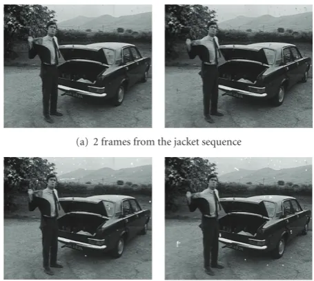
(a) 2 frames from the jacket sequence

(b) Frames with blotches highlighted in white

Figure 7: The second ground truth sequence is the “jacket” sequence. As the person in the sequence removes his jacket, the motion of the jacket is pathological and is an example of nonrigid object motion. This sequence has a higher blotch frequency than the “dance” sequence.

useful property of dirt is that it is opaque to IR and as a result is associated with low intensities in the transparency map. In the “dance” sequence a ground truth is estimated for 125 frames of 720×576 pixels. The ground truth is obtained by applying a threshold of 150 to each 8-bit transparency map.

Using IR scans is a good way to automatically generate a ground truth for dirt. However, there are a number of drawbacks to using IR scans. IR scans detect dirt even when dirt intensities are similar to the true image intensity. Such dirt cannot be detected by image-based missing data detectors. IR scans will also detect nonimpulsive dirt such as line scratches. As a result of these factors, the reported correct detection rate will be lower than the effective rate.

Table3: The experimental parameter values for the algorithm.

Parameter Value

Number of multiresolution levels 4

Number of iterations at each level 20

α2,α3 See (9)

Outer threshold Ratio,αr 0.5

Divergence weight,Λd 1

Divergence measure threshold,et 50

Roll-offrate,r 0.5

Spatial smoothness weight,Λd 1

PM bias,K 5

marked, allowing for a more realistic ground truth. A ground truth for 22 frames of the “jacket” sequence (seeFigure 7) was generated in this manner. The resolution of this sequence is also 720×576. The motion of the jacket is an example of the erratic motion of nonrigid bodies. This sequence also has a higher frequency of blotches than the “dance” sequence.

5.2. Experimental procedure

5.2.1. Motion estimation

The gradient-based motion estimator described by Kokaram in [13] is used to generate motion vectors for all the test sequences. The block size of vector field is 17×17 pixels with a 2 pixel horizontal and vertical overlap.

5.2.2. Configuration of the proposed algorithm

The key parameter of the algorithm is the deterministic thresholdδt which is used as the control parameter for the

ROC plots. The chosen values of δt are {5, 7, 9, 11, 13, 15,

17.5, 20, 25, 30, 35, 40}. These values are also used for the equivalent thresholds in the other missing data detectors used in the comparison outlined in Section 5.4, ensuring that each detector is detected over an equivalent range. The model error σ2

e is estimated before the first stage at each

multiresolution level by finding the variance of the four DFDs when s(x) = 0. The other relevant parameters are defined inTable 3.

5.2.3. ROC plots

The ROC curves are generated by finding the average correct detection and false alarm rates over all the frames of the test sequences for each value ofδt. The missing data correct

detection rate,rc, and false alarm rate,rf, are estimated for

each frame (and for eachδt), and are given by

rc=

xbgt(x)bdet(x)

xbgt(x)

,

rf =

x

1−bgt(x)bdet(x)

x

1−bgt(x) ,

(20)

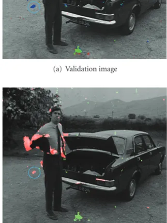
(a) Validation image

(b) PM/blotch detection

Figure8: This figure shows a validation image and a PM/blotch detection for the “jacket” sequence (correct detections—green, missed detections—blue, false alarms—red). The PM/blotch (red/ green) images can be used to indicate whether or not a missed blotch detection occurs to the pixel being detected as PM (blue circle).

wherebgt(x) is the binary ground truth blotch mask for the frame andbdet(x) is the binary output of the blotch detector under test. The curve is a parametric plot of corresponding (rc,rf) pairs.

5.2.4. PM rate plots

Plots of PM rate,rp, against the DFD thresholdδt are

eval-uated by finding the average relative frequency of PM in a sequence at each threshold. The PM rate is given by

rp=

xl(x)=2 x1

, (21)

where PM occurs whenl(x)=2.

5.2.5. Visual evaluation

Two types of image are used for the visual evaluation. They are validation images and PM/blotch detections (see

(a) A frame from the “dance” sequ-ence

(b) Configuration after determinis-tic initialisation

(c) Final field at level 3 (6 iterations in total)

(d) Field after 1st iteration at Level 2 (7 iterations in total)

(e) Final field at Level 2 (12 itera-tions)

(f) Field after 1st iteration at Level 1 (13 iterations)

(g) Final field at Level 1 (32 itera-tions)

(h) Field after 1st iteration at full resolution (33 iterations)

(i) Field after final iteration (52 iterations)

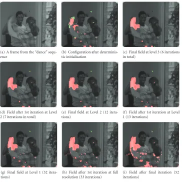
Figure9: This figure shows intermediate values of the label field (PM—Red, Blotches—Green) at various iterations of the ICM optimisation process for a frame from the “dance” sequence. The standard parameter set is used (Section 5.2) and the value ofδtis 7. Level 0 corresponds

to the full resolution; the resolution at level 1 is 360×288 and so on. At the coarsest resolution (Level 3) the resolution is 90×72 pixels.

(green), missed detections (blue), and false alarms (red). PM/blotch detections display the masks generated by the proposed algorithm and the Bornard algorithm with PM regions highlighted red and blotches highlighted green.

5.2.6. Implementation of the algorithm

The tests outlined on the proposed algorithm in this paper utilised a C++ implementation of the algorithm, incorporat-ing the IPP libraries [19] where appropriate. The algorithm was tested on a PC with a 1.4 Giga-Hertz Pentium M proc-essor with 1 Giga-Byte of RAM.

5.3. Algorithm evaluation

Figure 9gives an example of the evolution of the label field configuration for a frame of the “dance” sequence. Detection of missing data and PM at the coarser resolutions allows large PM and blotch features to be detected. As the resolution at which the optimisation occurs increases, the precision of the result increases, allowing small features to be detected. In

general, convergence at the coarser levels is fast as spatial information propagates quickly through the field, but as the resolution increases the speed of convergence decreases. In the example shown in Figure 9, the convergence occurs after six iterations at both Level 3 and Level 2. At the finer resolutions of Level 1 and Level 0, the maximum iteration limit of twenty iterations is reached. Computation time for this example is approximately ten seconds.

Applying the algorithm to all the frames of the test sequences gives the ROC and PM rate curves shown in

Figure 10. Overall, the maximum correct detection rates,rc,

for both sequences are quite low (approximately 25% for the “dance” sequence and 40% for the “jacket” sequence). However, there is also a low false alarm rate,rf, which does

not increase above 0.1% (roughly 400 pixels in a 720×576 image) even at low threshold values. The PM rate plots for both test sequences (Figures10(b)and10(d)) show that the rate of PM detection increases exponentially asδtdecreases.

10−2

10−3

10−4

False alarm rate,rf

0 0.1 0.2 0.3 0.4 0.5

C

o

rr

ect

d

et

ectio

n

ra

te

,

rc

(a) ROC for the “dance” sequence

40 35 30 25 20 15 10 5

δt

0 0.05 0.1 0.15 0.2 0.25

PM

det

ection

rat

e,

rp

(b) PM rate curve for the “dance” sequence

10−3

10−4

False alarm rate,rf

0 0.1 0.2 0.3 0.4 0.5 0.6

C

o

rr

ect

d

et

ectio

n

ra

te

,

rc

(c) ROC for the “jacket” sequence

40 35 30 25 20 15 10 5

δt

0 0.2 0.4 0.6 0.8 1

PM

det

ection

rat

e,

rp

(d) PM rate curve for the “jacket” sequence

Figure10: This figure shows ROC and PM rate plots (rpversusδt) for both test sequences obtained from the proposed algorithm using the

standard set of parameters.

trend in an ROC plot of a blotch detector is to have low correct detection and false alarm rates at higher threshold values and for the rates to increase as the value of the threshold drops, tending to a notional correct detection and false alarm rate of 100% at a zero threshold when every pixel in the image is detected as a blotch. The lowest value of the threshold used therefore gives the highest false alarm and correct detection rate. However, the ROC curves show that this pattern does not apply to the proposed algorithm. While the expected pattern is followed at high values of the thresholdδt, at lower values of the threshold a value is

reached, below which the correct detection rate no longer increases and continues to drop off. Although the rate at which temporal discontinuities are detected in the five-frame window continues to increase, an increasing number of pixels are classified as PM (seeFigure 11) since the likelihood of temporal discontinuities at the same location between

multiple frames greatly increases. This is confirmed by the exponentially increasing PM rate at lower threshold values. Consequently, less pixels are detected as missing data and the correct detection rate decreases. For this detector, the notional false alarm rate and correct detection rate at the zero threshold level is 0% as all pixels will be detected as pathological motion.

5.4. Comparison with other missing data detectors

The proposed algorithm is compared with five existing miss-ing data detectors. These include four conventional algo-rithms and the Bornard missing data detection algorithm [9]. The four other algorithms are the SDIp algorithm [2,

(a) Validation image forδt=5 (b) Validation image forδt=7

(c) PM/blotch detection forδt=5 (d) PM/blotch detection forδt=7 Figure11: This figure illustrates how lowering the DFD threshold

δtresults in a lower correct detection rate. The blue circle highlights

a large blotch which is not detected at the lower threshold ((a) and (b)—correct detections in green, missed detections in blue). At the lower threshold this blotch is classified as PM ((c) and (d)—red for PM, green for blotches).

5.4.1. Detector configuration

Both the SDIp and sROD algorithms have one associated parameterδtand are implemented directly from the

descrip-tion of the algorithms. The four probabilistic algorithms are implemented with as similar parameter values as possible. A multiresolution framework is employed for each algorithm, with a maximum of twenty iterations per level. An eight-pixel first-order spatial neighbourhood is used for either the blotch field (blotch MRF algorithm), the temporal dis-continuity field (TDFs) (Morris/Bornard algorithms) or the blotch/PM field (the proposed algorithm). The Bornard algorithm also employs a two-pixel temporal neighbourhood linking the TDFs. Like the proposed algorithm, in the Blotch MRF algorithm a smoothness prior is only enforced on the blotch field and not on the state field.

The value of the spatial smoothness weight in the Morris and Bornard algorithms is 1, and the temporal prior weight of the Bornard algorithm,β3, is−0.1. This reflects the setup recommended by Bornard in his thesis [9, Section 5.7.1.2], where the temporal prior weight is roughly one tenth the size of the spatial weight with a negative value. The search radius in the interpretation stage is 20 pixels with a temporal discontinuity threshold of 1. Although less conservative than the recommended setup (a radius of 38 pixels), PM will be flagged if a temporal discontinuity exists in one of 2×202π pixels which is approximately two and a half thousand pixels. For the proposed algorithm, the standard set of parameters described inSection 5.2is applied.

100

10−2

10−4

10−6

False alarm rate,rf

0 0.2 0.4 0.6 0.8 1

C

o

rr

ect

d

et

ectio

n

ra

te

,

rc

SDIp sROD Morris

Blotch MRF Bornard Blotch/PM MRF (a) ROC for the “dance” sequence

100

10−1

10−2

10−3

10−4

10−5

False alarm rate,rf

0 0.2 0.4 0.6 0.8 1

C

o

rr

ect

d

et

ectio

n

ra

te

,

rc

SDIp sROD Morris

Blotch MRF Bornard Blotch/PM MRF (b) ROC for the “jacket” sequence

Figure12: This figure shows the ROC curves for the 6 detectors under test for each test sequence. The standard parameter set is used for the proposed algorithm. The set up of each detector is described inSection 5.2.

5.4.2. Comparison with the conventional detectors

ROC curves are plotted for each detector, with the same set of values of δt as before (δt = {5, 7, 9, 11, 13, 15, 17.5, 20,

(a) Validation image for the blotch MRF detector (green—correct detections, red— false alarms, blue—missing data)

(b) Validation image for the proposed algo-rithm

(c) PM/blotch detection for the proposed algorithm (red—PM, green—blotches)

Figure13: This figure consists of validation images for the blotch MRF algorithm and the proposed algorithm for a frame from the “jacket” sequence. The value of the DFD threshold,δt, is 15. Also shown is the PM/blotch detection for the proposed algorithm. The blue square

highlights the region of the image where the proposed algorithm eliminates false alarms caused by pathological motion. The yellow circles highlight missed blotch detections in the proposed algorithm, which have been wrongly detected as PM.

(a) Validation image for the blotch MRF detector (green—correct detections, red— false alarms, blue—missing data)

(b) Validation image for the proposed algo-rithm

(c) PM/blotch detection for the proposed algorithm (red—PM, green—blotches)

Figure14: This figure consists of validation images for the blotch MRF algorithm and the proposed algorithm for a frame from the “dance” sequence, as well as the corresponding PM/blotch detection for the proposed algorithm. The value of the DFD threshold,δt, is 15. Using the

proposed algorithm reduces the number of false alarms in the region of the head of the female dancer.

(a) A frame from the “dance” se-quence

(b) A PM/blotch (red/green) de-tection for the frame (δt=11) Figure15: This blue circle in the two images highlights a blotch located near a region of motion blur. Due to its location the blotch is detected as PM by the proposed algorithm.

detectors, although the correct detection rates are also reduced. At higher values of the DFD threshold δt (i.e.,

before the maximum correct detection rate is reached), the

false alarm rate of the proposed algorithm is 75% to 90% less for the “dance” sequence and 50% to 80% less for the “jacket” sequence. On the other hand, both the Bornard and proposed algorithms have an upper limit on the rate of correct blotch detections. The average maximum correct detection rate of the proposed algorithm is two to three times less than the correct detection rates at the lowest threshold tested (δt=5), although the false alarm rate is 30 to 50 times

lower.

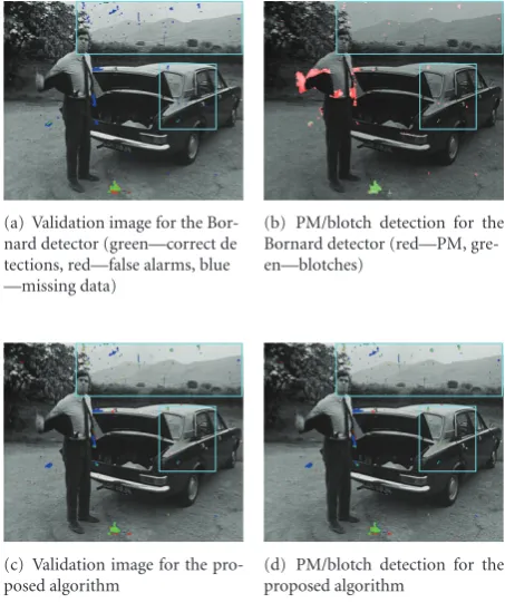
(a) Validation image for the Bor-nard detector (green—correct de tections, red—false alarms, blue —missing data)

(b) PM/blotch detection for the Bornard detector (red—PM, gre-en—blotches)

(c) Validation image for the pro-posed algorithm

(d) PM/blotch detection for the proposed algorithm

Figure 16: This figure illustrates the superior blotch detection rate of the proposed algorithm over the Bornard algorithm in the “jacket” sequence. The highlighted regions of the frame indicate blotches missed by the Bornard algorithm (image (a)) that are detected by the proposed algorithm (c). The blotches missed by the Bornard algorithm are detected as PM (b). The value ofδtused to

generate the images in this figure is 15.

consequence of the algorithm design, which is encouraged to maintain image quality rather than remove the maximum number of blotches. The second major cause of missed detec-tions occurs because of a high frequency of blotches over a number of frames. A fundamental assumption made by missing data detectors is that blotches are rarely located at the same spatial location in neighbouring frames. However, if there is a high frequency of blotches in a sequence, then the probability of blotches occurring at the same location in neighbouring frames increases. In such situations, a blotch is likely to be incorrectly classified as pathological motion.

5.4.3. Comparison with the Bornard algorithm

The missing data ROC curves inFigure 12also highlight the variable performance of the proposed algorithm when com-pared with the Bornard algorithm. The Bornard algorithm generally performs better on the “dance” sequence. At high thresholds, the false alarm rate,rf, of the Bornard algorithm

is lower for similar correct detection rates, rc. However,

at lower threshold values the difference in the false alarm rates decreases and the proposed algorithm achieves a higher maximum correct detection rate. On the other hand, the proposed algorithm is much more effective on the “jacket” sequence and achieves a much higher blotch detection rate.

The maximum correct detection rate is approximately 40%, roughly twice the maximum correct detection rate of the Bornard algorithm.

The poor correct detection rates of the Bornard algo-rithm on the “jacket” is clearly visible in the frame from the “jacket” sequence highlighted inFigure 16. Many of the blotches in the frame are detected as PM by the Bornard algorithm, caused by the high frequency of visible blotches in the sequence. The proposed algorithm is less prone to missed detections in such circumstances.

It is reasonable to conclude that the Bornard detector is more conservative than the proposed algorithm. The inter-pretation stage of the Bornard is more conservative than the cumulative effect of the divergence likelihood, the PM bias, and the outer threshold ratio. The interpretation stage acts as a “maximum caution” classifier, rejecting any candidate blotch site if a single temporal discontinuity exists within a radius (20 pixels) of the candidate in either of the outer temporal discontinuity fields. The ultra-cautious nature of the interpretation allows the Bornard detector to achieve lower false alarm rates. However, it also results in more missed detections at lower threshold values or when there is a high frequency of blotches in a sequence.

On the other hand, the proposed algorithm tries to make an informed decision and as such is less indiscriminate than the Bornard algorithm. For a site to be detected as PM rath-er than a blotch, the proposed algorithm requires eithrath-er a temporal discontinuity to exist in at least one outer tem-poral discontinuity field at the same location or spatial prop-agation from neighbouring PM sites by means of the smoo-thness prior. The divergence likelihood, the PM bias, and the outer threshold are all intended to make the proposed algorithm more likely to detect PM. The divergence likeli-hood increases the probability of sites with high motion field divergences being detected as PM, the PM bias encourages the spatial propagation of PM states and the outer threshold ratio increases the likelihood of temporal discontinuities being detected in the outer fields.

5.5. Blotch restoration using the proposed algorithm

The critical design criterion of the proposed algorithm is that it eliminates image damage during missing data treat-ment. A primitive missing data treatment algorithm was im-plemented that takes a blotch mask from any detector and interpolates detected blotches with the mean motion com-pensated intensity of the previous and next frames.

Figure 17 compares images restored using both the blotch MRF algorithm and the proposed algorithm (δt =

(a) From left to right, frames from the “jacket,” “vj,” “birds,” and “chopper” sequences

(b) PM/blotch detections of the four frames for the proposed algorithm

(c) Frames restored with the Blotch MRF algorithm

(d) Frames restored with the proposed algorithm

Figure17: This figure shows frames from four sequences restored using the Blotch MRF and proposed algorithms as blotch detectors. The highlighted frames show image damage present if the Blotch MRF is used instead of the proposed algorithm.

sequence (the “chopper” sequence) contains an example of motion blur. The rotation of the rotors is also an issue, as the motion estimator employs a purely translational motion model.

The four examples shown in Figure 17 highlight the effectiveness of the proposed algorithm. Using the proposed algorithm prevents significant damage to each of the four images shown. However, the proposed algorithm is not al-ways able to prevent all image damage, especially in cases where the region of PM is undergoing a translation (i.e., the motion of an object is the sum of PM and a nonpathological translation (see Figure 18)). The assumption is made that motion compensation can be performed accurately, even in regions of PM. Consequently, the algorithm is prone to failure as it involves the motion compensation of four frames with respect to the central frame. However, it should also be

noted that while some image damage may occur, any damage will be much less than the damage caused by performing missing data treatment without detection of PM.

5.6. Computational complexity

Estimation of the prior energy and estimation of the MAP state at each pixel is the most computationally intensive aspect of the algorithm, amounting to approximately 90% of the execution time for a single frame. The upper bound for the complexity of the ICM optimisation isO(# iterations×

(a) A frame from the “birds” seq-uence

(b) Restored frame Figure18: This figure shows an example from the “birds” sequence where the proposed algorithm fails to prevent damage to image data (the highlighted regions). In this example, the object (the bird) undergoing PM is also undergoing a translation. This motion causes the algorithm to fail on some frames but not others.

of iterations necessary for convergence also depends on the number of states and the size of the neighbourhood, with a higher number of states and greater neighbourhood size requiring more iterations for convergence. From observation of the algorithm, the size of theδtthreshold also impacts on

the number of iterations required. The average number of iterations performs decreases asδt increases. Computation

time varies between 5 and 15 seconds per frame, depending on the number iterations performed.

Further reductions in computation would be possible by reducing the complexity of the probabilistic model. For example, the model could be approximated by reducing the number of labels in l(x) to two (i.e., missing data or not missing data) and by using a mixture model to approximate the data likelihood distributions. This would also allow a graph cuts [20] based segmentation to be performed.

6. FINAL COMMENTS

This paper has presented a new robust missing data detection algorithm that aims to reduce false alarms due to patho-logical motion. It uses a probabilistic framework to detect regions of PM, preventing them from being detected as blotches. A quantitative comparison of the algorithm was presented, comparing the algorithm against four standard blotch detectors and the Bornard PM detection algorithm. The comparison showed that the proposed algorithm gives a significantly reduced false alarm rate when compared with the standard detectors. Although a lower false alarm rate can be obtained with the Bornard algorithm at high thresholds, higher correct detection rates are possible with the proposed algorithm. A further visual evaluation of the algorithm shows how the algorithm can prevent image damage when used as a detector in a missing data treatment framework.

However, the proposed algorithm does not address how the image is to be restored in PM regions. The missing data algorithms outlined in this paper will fail in these regions. Restoration in PM regions has been a topic touched on by Rares in [11] in which an alternative metric for detecting blotches in PM was proposed. As temporal reconstruction of missing data in PM regions is unreliable, spatial

reconstruc-tion techniques are necessary such as image inpainting [21] or texture synthesis [22].

The major area of further development in this area would be to integrate the algorithm into a missing data treatment framework. The algorithm outlined in this paper is presented as a stand-alone blotch detector which operates independently of a missing data interpolation stage. Previous work in missing data treatment [10, 23, 24] has shown that integrating the detection, interpolation, and motion estimation stages into a single Bayesian framework allows for a more visually pleasing restoration. A new missing data treatment algorithm along the lines of the JONDI algorithm [24] using the proposed algorithm for the detection stage could result in an integrated framework resistant to patho-logical motion.

ACKNOWLEDGMENTS

This work has been supported by the Irish Research Council for Science Engineering and Technology’s Embark initiative, the Adobe corporation, the European Union (EU) Pres-tospace project, and the European Marie Curie Transfer of Knowledge project Axiom.

REFERENCES

[1] A. Kokaram,Motion Picture Restoration: Digital Algorithms for Artefact Suppression in Degraded Motion Picture Film and Video, chapter 6, Springer, New York, NY, USA, 1998. [2] A. Kokaram, R. D. Morris, W. J. Fitzgerald, and P. J. W.

Rayner, “Detection of missing data in image sequences,”IEEE Transactions on Image Processing, vol. 4, no. 11, pp. 1496–1508, 1995.

[3] M. J. Nadenau and S. K. Mitra, “Blotch and scratch detection in image sequences based on rank order differences,” in Proceedings of the 5th International Workshop on Time-Varying Image Processing and Moving Object Recognition, Florence, Italy, September 1996.

[4] J. Biemond, P. M. B. van Roosmalen, and R. L. Lagendijk, “Improved blotch detection by postprocessing,” inProceedings of the International Conference on Acoustics, Speech, and Signal Processing (ICASSP ’99), vol. 6, pp. 3101–3104, Phoenix, Ariz, USA, March 1999.

[5] R. D. Morris, “Image sequence distribution using Gibbs distri-butions,” Ph.D. thesis, Cambridge University, Cambridge, UK, 1995.

[6] B. Kent, A. Kokaram, B. Collis, and S. Robinson, “Two layer segmentation for handling pathological motion in degraded post production media,” inProceedings of IEEE International Conference on Image Processing (ICIP ’04), vol. 1, pp. 299–302, Singapore, October 2004.

[7] J. Ren and T. Vlachos, “Dirt detection for archive film restoration using an adaptive spatio-temporal approach,” in Proceedings of the 2nd European IEE Conference on Visual Media Production (CVMP ’05), pp. 221–230, London, UK, November 2005.

[9] R. Bornard, “Probabilistic approaches for the digital restora-tion of television archives,” Ph.D. thesis, Ecole Centrale Paris, Paris, France, 2002.

[10] A. Kokaram and S. J. Godsill, “MCMC for joint noise reduc-tion and missing data treatment in degraded video,” IEEE Transactions on Signal Processing, vol. 50, no. 2, pp. 189–205, 2002.

[11] A. Rares, M. J. T. Reinders, and J. Biemond, “Complex event classification in degraded image sequences,” inProceedings of IEEE International Conference on Image Processing (ICIP ’01), vol. 1, pp. 253–256, Thessaloniki, Greece, October 2001. [12] P. M. B. van Roosmalen, “Restoration of archived film and

video,” Ph.D. thesis, Delft University of Technology, Delft, The Netherlands, 1999.

[13] A. Kokaram, Motion Picture Restoration: Digital Algorithms for Artefact Suppression in Degraded Motion Picture Film and Video, chapter 2, Springer, New York, NY, USA, 1998. [14] J. Konrad and E. Dubois, “Bayesian estimation of motion

vec-tor fields,”IEEE Transactions on Pattern Analysis and Machine Intelligence, vol. 14, no. 9, pp. 910–927, 1992.

[15] J. E. Besag, “On the statistical analysis of dirty pictures,” Journal of the Royal Statistical Society B, vol. 48, no. 3, pp. 259– 302, 1986.

[16] F. Heitz, P. Perez, and P. Bouthemy, “Multiscale minimization of global energy functions in some visual recovery problems,” CVGIP: Image Understanding, vol. 59, no. 1, pp. 125–134, 1994.

[17] Institut national de l’audiovisuel,http://www.ina.fr/index.en .html.

[18] “Prestospace: an integrated solution for audio-visual preserva-tion and access,”http://www.prestospace.org/.

[19] Intel performance primitive (ipp) libraries,http://www.intel .com/cd/software/products/asmo-na/eng/302910.htm. [20] Y. Y. Boykov and M.-P. Jolly, “Interactive graph cuts for

optimal boundary & region segmentation of objects in N-D images,” inProceedings of the 8th IEEE International Conference on Computer Vision (ICCV ’01), vol. 1, pp. 105–112, Vancou-ver, Canada, July 2001.

[21] A. Rares, M. J. T. Reinders, and J. Biemond, “Edge-based image restoration,”IEEE Transactions on Image Processing, vol. 14, no. 10, pp. 1454–1468, 2005.

[22] A. A. Efros and T. K. Leung, “Texture synthesis by non-parametric sampling,” inProceedings of the 7th IEEE Interna-tional Conference on Computer Vision (ICCV ’99), vol. 2, pp. 1033–1038, Kerkyra, Greece, September 1999.

[23] A. Kokaram, Motion Picture Restoration: Digital Algorithms for Artefact Suppression in Degraded Motion Picture Film and Video, chapter 7, Springer, New York, NY, USA, 1998. [24] A. Kokaram, “On missing data treatment for degraded video