SemEval-2015 Task 10: Sentiment Analysis in Twitter
Sara Rosenthal Columbia University
Saif M Mohammad National Research Council Canada
Preslav Nakov
Qatar Computing Research Institute
Alan Ritter The Ohio State University
Svetlana Kiritchenko National Research Council Canada
Veselin Stoyanov Facebook
Abstract
In this paper, we describe the 2015 iteration of the SemEval shared task on Sentiment Analy-sis in Twitter. This was the most popular sen-timent analysis shared task to date with more than 40 teams participating in each of the last three years. This year’s shared task competi-tion consisted of five sentiment prediccompeti-tion sub-tasks. Two were reruns from previous years: (A) sentiment expressed by a phrase in the context of a tweet, and (B) overall sentiment of a tweet. We further included three new sub-tasks asking to predict (C) the sentiment to-wards a topic in a single tweet, (D) the over-all sentiment towards a topic in a set of tweets, and (E) the degree of prior polarity of a phrase.
1 Introduction
Social media such as Weblogs, microblogs, and dis-cussion forums are used daily to express personal thoughts, which allows researchers to gain valuable insight into the opinions of a very large number of individuals, i.e., at a scale that was simply not pos-sible a few years ago. As a result, nowadays, sen-timent analysis is commonly used to study the pub-lic opinion towards persons, objects, and events. In particular, opinion mining and opinion detection are applied to product reviews (Hu and Liu, 2004), for agreement detection (Hillard et al., 2003), and even for sarcasm identification (Gonz´alez-Ib´a˜nez et al., 2011; Liebrecht et al., 2013).
Early work on detecting sentiment focused on newswire text (Wiebe et al., 2005; Baccianella et al., 2010; Pang et al., 2002; Hu and Liu, 2004). As later research turned towards social media, people real-ized this presented a number of new challenges.
Misspellings, poor grammatical structure, emoti-cons, acronyms, and slang were common in these new media, and were explored by a number of re-searchers (Barbosa and Feng, 2010; Bifet et al., 2011; Davidov et al., 2010; Jansen et al., 2009; Kouloumpis et al., 2011; O’Connor et al., 2010; Pak and Paroubek, 2010). Later, specialized shared tasks emerged, e.g., at SemEval (Nakov et al., 2013; Rosenthal et al., 2014), which compared teams against each other in a controlled environment us-ing the same trainus-ing and testus-ing datasets. These shared tasks had the side effect to foster the emer-gence of a number of new resources, which eventu-ally spread well beyond SemEval, e.g., NRC’s Hash-tag Sentiment lexicon and the Sentiment140 lexicon (Mohammad et al., 2013).1
Below, we discuss the public evaluation done as part of SemEval-2015 Task 10. In its third year, the SemEval task on Sentiment Analysis in Twitter has once again attracted a large number of participants: 41 teams across five subtasks, with most teams par-ticipating in more than one subtask.
This year the task included reruns of two legacy subtasks, which asked to detect the sentiment ex-pressed in a tweet or by a particular phrase in a tweet. The task further added three new subtasks. The first two focused on the sentiment towards a given topic in a single tweet or in a set of tweets, respectively. The third new subtask focused on de-termining the strength of prior association of Twit-ter Twit-terms with positive sentiment; this acts as an in-trinsic evaluation of automatic methods that build Twitter-specific sentiment lexicons with real-valued sentiment association scores.
1http://www.purl.com/net/lexicons
In the remainder of this paper, we first introduce the problem of sentiment polarity classification and our subtasks. We then describe the process of creat-ing the traincreat-ing, development, and testcreat-ing datasets. We list and briefly describe the participating sys-tems, the results, and the lessons learned. Finally, we compare the task to other related efforts and we point to possible directions for future research.
2 Task Description
Below, we describe the five subtasks of SemEval-2015 Task 10 on Sentiment Analysis in Twitter.
• Subtask A. Contextual Polarity Disambigua-tion: Given an instance of a word/phrase in the context of a message, determine whether it ex-presses a positive, a negative or a neutral senti-ment in that context.
• Subtask B. Message Polarity Classification:
Given a message, determine whether it expresses a positive, a negative, or a neutral/objective senti-ment. If both positive and negative sentiment are expressed, the stronger one should be chosen.
• Subtask C. Topic-Based Message Polarity Classification: Given a message and a topic, de-cide whether the message expresses a positive, a negative, or a neutral sentiment towards the topic. If both positive and negative sentiment are ex-pressed, the stronger one should be chosen.
• Subtask D. Detecting Trend Towards a Topic:
Given a set of messages on a given topic from the same period of time, classify the overall sen-timent towards the topic in these messages as (a) strongly positive, (b) weakly positive, (c) neu-tral, (d) weakly negative, or (e) strongly negative.
• Subtask E. Determining Strength of Associa-tion of Twitter Terms with Positive Sentiment (Degree of Prior Polarity):Given a word/phrase, propose a score between 0 (lowest) and 1 (high-est) that is indicative of the strength of association of that word/phrase with positive sentiment. If a word/phrase is more positive than another one, it should be assigned a relatively higher score.
3 Datasets
In this section, we describe the process of collect-ing and annotatcollect-ing our datasets of short social me-dia text messages. We focus our discussion on the 2015 datasets; more detail about the 2013 and the 2014 datasets can be found in (Nakov et al., 2013) and (Rosenthal et al., 2014).
3.1 Data Collection 3.1.1 Subtasks A–D
First, we gathered tweets that express sentiment about popular topics. For this purpose, we ex-tracted named entities from millions of tweets, us-ing a Twitter-tuned NER system (Ritter et al., 2011). Our initial training set was collected over a one-year period spanning from January 2012 to January 2013. Each subsequent Twitter test set was collected a few months prior to the corresponding evaluation. We used the public streaming Twitter API to download the tweets.
We then identified popular topics as those named entities that are frequently mentioned in association with a specific date (Ritter et al., 2012). Given this set of automatically identified topics, we gathered tweets from the same time period which mentioned the named entities. The testing messages had differ-ent topics from training and spanned later periods.
The collected tweets were greatly skewed towards the neutral class. In order to reduce the class im-balance, we removed messages that contained no sentiment-bearing words using SentiWordNet as a repository of sentiment words. Any word listed in SentiWordNet 3.0 with at least one sense having a positive or a negative sentiment score greater than 0.3 was considered a sentiment-bearing word.2
For subtasks C and D, we did some manual prun-ing based on the topics. First, we excluded top-ics that were incomprehensible, ambiguous (e.g., Barcelona, which is a name of a sports team and also of a place), or were too general (e.g.,Paris, which is a name of a big city). Second, we discarded tweets that were just mentioning the topic, but were not re-ally about the topic. Finre-ally, we discarded topics with too few tweets, namely less than 10.
Instructions: Subjective words are ones which convey an opinion or sentiment. Given a Twitter message, identify whether it is objective, positive, negative, or neutral. Then, identify each subjective word or phrase in the context of the sentence and mark the position of its start and end in the text boxes below. The number above each word indicates its position. The word/phrase will be generated in the adjacent textbox so that you can confirm that you chose the correct range. Choose the polarity of the word or phrase by selecting one of the radio buttons: positive, negative, or neutral. If a sentence is not subjective please select the checkbox indicating that “There are no subjective words/phrases”. If a tweet is sarcastic, please select the checkbox indicating that “The tweet is sarcastic”. Please read the examples and invalid responses before beginning if this is your first time answering this hit.
Figure 1: The instructions we gave to the workers on Mechanical Turk, followed by a screenshot.
3.1.2 Subtask E
We selected high-frequency target terms from the Sentiment140 and the Hashtag Sentiment tweet cor-pora (Kiritchenko et al., 2014). In order to re-duce the skewness towards the neutral class, we selected terms from different ranges of automati-cally determined sentiment values as provided by the corresponding Sentiment140 and Hashtag Sen-timent lexicons. The term set comprised regular En-glish words, hashtagged words (e.g., #loveumom), misspelled or creatively spelled words (e.g., parla-ment orhappeeee), abbreviations, shortenings, and slang. Some terms were negated expressions such as no fun. (It is known that negation impacts the sentiment of its scope in complex ways (Zhu et al., 2014).) We annotated these terms for degree of sen-timent manually. Further details about the data col-lection and the annotation process can be found in Section 3.2.2 as well as in (Kiritchenko et al., 2014). The trial dataset consisted of 200 instances, and no training dataset was provided. Note, however, that the trial data was large enough to be used as a development set, or even as a training set. More-over, the participants were free to use any additional manually or automatically generated resources when building their systems for subtask E. The testset in-cluded 1,315 instances.
3.2 Annotation
Below we describe the data annotation process.
3.2.1 Subtasks A–D
We used Amazon’s Mechanical Turk for the an-notations of subtasks A–D. Each tweet message was annotated by five Mechanical Turk workers, also known as Turkers. The annotations for subtasks A–D were done concurrently, in a single task. A Turker had to mark all the subjective words/phrases in the tweet message by indicating their start and end positions and to say whether each subjective word/phrase was positive, negative, or neutral (sub-task A). He/she also had to indicate the overall po-larity of the tweet message in general (subtask B) as well as the overall polarity of the message to-wards the given target topic (subtasks C and D). The instructions we gave to the Turkers, along with an example, are shown in Figure 1. We further made available to the Turkers several additional examples, which we show in Table 1.
Authorities areonly too awarethat Kashgar is 4,000 kilometres (2,500 miles) from Beijing butonlya tenth of the distance from the Pakistani border, and aredesperatetoensure instability or militancydoes not leak over the frontiers.
Taiwan-made productsstood a good chanceof becomingeven more competitive thanks towider access to overseas markets and lower costs for material imports, he said.
“Marchappearsto be amore reasonableestimate while earlier admissioncannot be entirely ruled out,” according to Chen, also Taiwan’s chief WTO negotiator.
friday evening plans were great, but saturday’s plansdidnt go as expected– i went dancing & it was anokclub, butterribly crowded :-(
WHY THEHELLDO YOU GUYS ALL HAVE MRS. KENNEDY! SHES A FUCKING DOUCHE
AT&T wasokaybut whenever they do somethingnicein the name of customer service it seems like a favor, while T-Mobile makes that anormal everyday thin
obama should beimpeachedonTREASONcharges. Our Nuclear arsenal was TOP Secret. Till HE told our enemies what we had.#Coward #Traitor
My graduation speech: “I’d like tothanksGoogle, Wikipedia and my computer!”:D#iThingteens
Table 1: List of example sentences and annotations we provided to the Turkers. All subjective phrases are italicized and color-coded: positive phrases are in green, negative ones are in red, and neutral ones are in blue.
I would loveto watch Vampire Diaries:)and some Heroes!Great combination 9/13 I would love to watch Vampire Diaries :) and someHeroes! Greatcombination 11/13 Iwould loveto watch Vampire Diaries:)and some Heroes!Greatcombination 10/13 I wouldloveto watch Vampire Diaries :) and some Heroes!Greatcombination 13/13 I would love to watch Vampire Diaries :) and some Heroes!Greatcombination 12/13 I wouldloveto watch Vampire Diaries :) and some Heroes!Greatcombination
Table 2: Example of a sentence annotated for subjectivity on Mechanical Turk. Words and phrases that were marked as subjective are in bold italic. The first five rows are annotations provided by Turkers, and the final row shows their intersection. The last column shows the token-level accuracy for each annotation compared to the intersection.
We further discarded the following types of mes-sage annotations:
• containing overlapping subjective phrases; • marked as subjective but having no annotated
subjective phrases;
• with every single word marked as subjective; • with no overall sentiment marked;
• with no topic sentiment marked.
Recall that each tweet message was annotated by five different Turkers. We consolidated these anno-tations for subtask A using intersection as shown in the last row of Table 2. A word had to appear in 3/5 of the annotations in order to be considered subjec-tive. It further had to be labeled with a particular polarity (positive, negative, or neutral) by three of the five Turkers in order to receive that polarity la-bel. As the example shows, this effectively shortens the spans of the annotated phrases, often to single words, as it is hard to agree on long phrases.
Corpus Pos. Neg. Obj. Total
/ Neu.
Twitter2013-train 5,895 3,131 471 9,497 Twitter2013-dev 648 430 57 1,135 Twitter2013-test 2,734 1,541 160 4,435 SMS2013-test 1,071 1,104 159 2,334 Twitter2014-test 1,807 578 88 2,473
Twitter2014-sarcasm 82 37 5 124
LiveJournal2014-test 660 511 144 1,315 Twitter2015-test 1899 1008 190 3097
Table 3: Dataset statistics for subtask A.
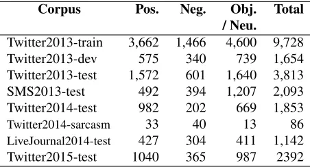
Corpus Pos. Neg. Obj. Total / Neu.
Twitter2013-train 3,662 1,466 4,600 9,728 Twitter2013-dev 575 340 739 1,654 Twitter2013-test 1,572 601 1,640 3,813 SMS2013-test 492 394 1,207 2,093 Twitter2014-test 982 202 669 1,853
Twitter2014-sarcasm 33 40 13 86
LiveJournal2014-test 427 304 411 1,142 Twitter2015-test 1040 365 987 2392
Table 4: Dataset statistics for subtask B.
Corpus Topics Pos. Neg. Obj. Total / Neu.
Train 44 142 56 288 530
[image:5.612.73.299.55.177.2]Test 137 870 260 1256 2386
Table 5: Twitter-2015 statistics for subtasks C & D.
For subtasks B and C, we consolidated the tweet-level annotations using majority voting, requiring that the winning label be proposed by at least three of the five Turkers; we discarded all tweets for which 3/5 majority could not be achieved. As in previous years, we combined the objective and the neutral la-bels, which Turkers tended to mix up.
We used these consolidated annotations as gold labels for subtasks A, B, C & D. The statistics for all datasets for these subtasks are shown in Tables 3, 4, and 5, respectively. Each dataset is marked with the year of the SemEval edition it was produced for. An annotated example from each source (Twitter, SMS, LiveJournal) is shown in Table 6; examples for sen-timent towards a topic can be seen in Table 7.
3.2.2 Subtask E
Subtask E asks systems to propose a numerical score for the positiveness of a given word or phrase. Many studies have shown that people are actually quite bad at assigning such absolute scores: inter-annotator agreement is low, and inter-annotators strug-gle even to remain self-consistent. In contrast, it is much easier to make relative judgments, e.g., to say whether one word is more positive than another. Moreover, it is possible to derive an absolute score from pairwise judgments, but this requires a much larger number of annotations. Fortunately, there are schemes that allow to infer more pairwise annota-tions from less judgments.
One such annotation scheme is MaxDiff (Lou-viere, 1991), which is widely used in market surveys (Almquist and Lee, 2009); it was also used in a pre-vious SemEval task (Jurgens et al., 2012).
In MaxDiff, the annotator is presented with four terms and asked which term is most positive and which is least positive. By answering just these two questions, five out of six pairwise rankings become known. Consider a set in which a judge evaluatesA, B,C, andD. If she says thatAandDare the most and the least positive, we can infer the following: A > B, A > C, A > D, B > D, C > D. The re-sponses to the MaxDiff questions can then be easily translated into a ranking for all the terms and also into a real-valued score for each term. We crowd-sourced the MaxDiff questions on CrowdFlower, re-cruiting ten annotators per MaxDiff example. Fur-ther details can be found in Section 6.1.2. of (Kir-itchenko et al., 2014).
3.3 Lower & Upper Bounds
Source Message Message-Level Polarity Twitter Why would you [still]- wear shorts when it’s this cold?! I [love]+ how Britain
[image:6.612.74.540.188.264.2]see’s a bit of sun and they’re [like ’OOOH]+ LET’S STRIP!’ positive SMS [Sorry]- I think tonight [cannot]- and I [not feeling well]- after my rest. negative LiveJournal [Cool]+ posts , dude ; very [colorful]+ , and [artsy]+ . positive Twitter Sarcasm [Thanks]+ manager for putting me on the schedule for Sunday negative
Table 6: Example annotations for each source of messages. The subjective phrases are marked in [. . .], and are followed by their polarity (subtask A); the message-level polarity is shown in the last column (subtask B).
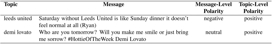
Topic Message Message-Level Topic-Level
Polarity Polarity leeds united Saturday without Leeds United is like Sunday dinner it doesn’t
feel normal at all (Ryan) negative positive
demi lovato Who are you tomorrow? Will you make me smile or just bring
me sorrow? #HottieOfTheWeek Demi Lovato neutral positive
Table 7: Example of annotations in Twitter showing differences between topic- and message-level polarity.
Corpus Subtask A Subtask B
Low Avg Up Avg
Twitter2013-train 75.1 89.7 97.9 77.6 Twitter2013-dev 66.6 85.3 97.1 86.4 Twitter2013-test 76.8 90.3 98.0 75.9 SMS2013-test 75.9 97.5 89.6 77.5 Livejournal2014-test 61.7 82.3 94.5 76.2 Twitter2014-test 75.3 88.9 97.5 74.7 Sarcasm2014-test 62.6 83.1 95.6 71.2 Twitter2015-test 73.2 87.6 96.8 75.7
Table 8: Average (over all HITs) overlap of the gold an-notations with the worst, average, and the worst Turker for each HIT, for subtasks A and B.
3.4 Tweets Delivery
Due to restrictions in the Twitter’s terms of service, we could not deliver the annotated tweets to the par-ticipants directly. Instead, we released annotation indexes and labels, a list of corresponding Twitter IDs, and a download script that extracts the corre-sponding tweets via the Twitter API.3
As a result, different teams had access to differ-ent number of training tweets depending on when they did the downloading. However, our analysis has shown that this did not have a major impact and many high-scoring teams had less training data com-pared to some lower-scoring ones.
3https://dev.twitter.com
4 Scoring
4.1 Subtasks A-C: Phrase-Level,
Message-Level, and Topic-Level Polarity
The participating systems were required to perform a three-way classification, i.e., to assign one of the folowing three labels: positive, negative or objec-tive/neutral. We evaluated the systems in terms of a macro-averagedF1score for predicting positive and
negative phrases/messages.
We first computed positive precision,Pposas fol-lows: we found the number of phrases/messages that a system correctly predicted to be positive, and we divided that number by the total number of examples it predicted to be positive. To com-pute positive recall,Rpos, we found the number of phrases/messages correctly predicted to be positive and we divided that number by the total number of positives in the gold standard. We then calcu-lated an F1 score for the positive class as follows
Fpos = 2PposRpos
Ppos+Rpos. We carried out similar
computa-tions for the negative phrases/messages,Fneg. The overall score was then computed as the average of the F1scores for the positive and for the negative
classes:F = (Fpos+Fneg)/2.
We provided the participants with a scorer that outputs the overall score F, as well as P, R, and F1 scores for each class (positive, negative, neutral)
4.2 Subtask D: Overall Polarity Towards a Topic
This subtask asks to predict the overall sentiment of a set of tweets towards a given topic. In other words, to predict the ratioriof positive (posi) tweets to the number of positive and negative sentiment tweets in the set of tweets about thei-th topic:
ri=P osi/(P osi+Negi)
Note, that neutral tweets do not participate in the above formula; they have only an indirect impact on the calculation, similarly to subtasks A–C.
We use the following two evaluation measures for subtask D:
• AvgDiff (official score): Calculates the abso-lute difference betweeen the predicted r0
i and the gold ri for each i, and then averages this difference over all topics.
• AvgLevelDiff(unofficial score): This calcula-tion is the same as AvgDiff, but with r0
i and ri first remapped to five coarse numerical cat-egories: 5 (strongly positive), 4 (weakly pos-itive), 3 (mixed), 2 (weakly negative), and 1 (strongly negative). We define this remapping based on intervals as follows:
– 5:0.8< x≤1.0 – 4:0.6< x≤0.8 – 3:0.4< x≤0.6 – 2:0.2< x≤0.4 – 1:0.0≤x≤0.2
4.3 Subtask E: Degree of Prior Polarity
The scores proposed by the participating systems were evaluated by first ranking the terms accord-ing to the proposed sentiment score and then com-paring this ranked list to a ranked list obtained from aggregating the human ranking annotations. We used Kendall’s rank correlation (Kendall’s τ) as the official evaluation metric to compare the ranked lists (Kendall, 1938). We also calculated scores for Spearman’s rank correlation (Lehmann and D’Abrera, 2006), as an unofficial score.
Team ID Affiliation
CIS-positiv University of Munich CLaC-SentiPipe CLaC Labs, Concordia University DIEGOLab Arizona State University ECNU East China Normal University elirf Universitat Polit`ecnica de Val`encia Frisbee Frisbee
Gradiant-Analytics Gradiant
GTI AtlantTIC Center, University of Vigo IHS-RD IHS inc
iitpsemeval Indian Institute of Technology, Patna IIIT-H IIIT, Hyderabad
INESC-ID IST, INESC-ID
IOA Institute of Acoustics, Chinese Academy of Sciences KLUEless FAU Erlangen-N¨urnberg
lsislif Aix-Marseille University
NLP NLP
RGUSentimentMiners123 Robert Gordon University RoseMerry The University of Melbourne Sentibase IIIT, Hyderabad
SeNTU Nanyang Technological University, Singapore SHELLFBK Fondazione Bruno Kessler
sigma2320 Peking University Splusplus Beihang University SWASH Swarthmore College SWATAC Swarthmore College SWATCMW Swarthmore College SWATCS65 Swarthmore College
Swiss-Chocolate Zurich University of Applied Sciences TwitterHawk University of Massachusetts, Lowell UDLAP2014 Universidad de las Am`ericas Puebla, Mexico UIR-PKU University of International Relations UMDuluth-CS8761 University of Minnesota, Duluth UNIBA University of Bari Aldo Moro unitn University of Trento UPF-taln Universitat Pompeu Fabra WarwickDCS University of Warwick Webis Bauhaus-Universit¨at Weimar
[image:7.612.321.530.58.351.2]whu-iss International Software School, Wuhan University Whu-Nlp Computer School, Wuhan University wxiaoac Hong Kong University of Science and Technology ZWJYYC Peking University
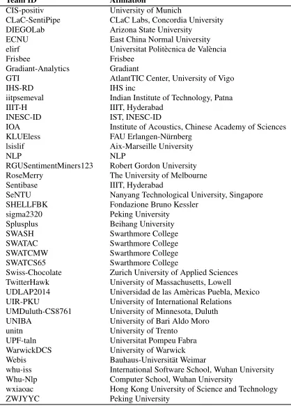
Table 9: The participating teams and their affiliations.
5 Participants and Results
The task attracted 41 teams: 11 teams participated in subtask A, 40 in subtask B, 7 in subtask C, 6 in sub-task D, and 10 in subsub-task E. The IDs and affiliations of the participating teams are shown in Table 9.
5.1 Subtask A: Phrase-Level Polarity
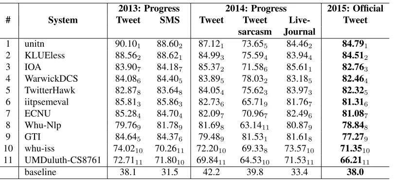
The results (macro-averaged F1 score) for
sub-task A are shown in Table 10. The official results on the new Twitter2015-test dataset are shown in the last column, while the first five columns show F1 on the 2013 and on the 2014
progress test datasets:4Twitter2013-test,
SMS2013-test, Twitter2014-SMS2013-test, Twitter2014-sarcasm, and LiveJournal2014-test. There is an index for each re-sult showing the relative rank of that rere-sult within the respective column. The participating systems are ranked by their score on the Twitter2015-test dataset, which is the official ranking for subtask A; all remaining rankings are secondary.
2013: Progress 2014: Progress 2015: Official
# System Tweet SMS Tweet Tweet Live- Tweet
sarcasm Journal
1 unitn 90.101 88.602 87.121 73.655 84.462 84.791
2 KLUEless 88.562 88.621 84.993 75.594 83.944 84.512
3 IOA 83.907 84.187 85.372 71.586 85.611 82.763
4 WarwickDCS 84.086 84.405 83.895 78.032 83.185 82.464
5 TwitterHawk 82.878 83.648 84.054 75.623 83.973 82.325
6 iitpsemeval 85.813 85.863 82.736 65.719 81.767 81.316
7 ECNU 85.284 84.704 82.097 70.967 82.496 81.087
8 Whu-Nlp 79.769 81.789 81.698 63.1411 80.879 78.848
9 GTI 84.645 84.376 79.489 81.531 81.618 77.279
10 whu-iss 74.0210 70.2611 72.2010 69.338 73.5710 71.3510
11 UMDuluth-CS8761 72.7111 71.8010 69.8411 64.5310 71.5311 66.2111
[image:8.612.106.511.52.237.2]baseline 38.1 31.5 42.2 39.8 33.4 38.0
Table 10:Results for subtask A: Phrase-Level Polarity.The systems are ordered by their score on the Twitter2015 test dataset; the rankings on the individual datasets are indicated with a subscript.
There were less participants this year, probably due to having a new similar subtask: C. Notably, many of the participating teams were newcomers.
We can see that all systems beat the majority class baseline by 25-40 F1 points absolute on all
datasets. The winning team unitn (using deep con-volutional neural networks) achieved anF1of 84.79
on Twitter2015-test, followed closely by KLUEless (using logistic regression) withF1=84.51.
Looking at the progress datasets, we can see that unitn was also first on both progress Tweet datasets, and second on SMS and on LiveJournal. KLUE-less won SMS and was second on Twitter2013-test. The best result on LiveJournal was achieved by IOA, who were also second on Twitter2014-test and third on the official Twitter2015-test. None of these teams was ranked in top-3 on Twitter2014-sarcasm, where the best team was GTI, followed by WarwickDCS.
Compared to 2014, there is an improvement on Twitter2014-test from 86.63 in 2014 (NRC-Canada) to 87.12 in 2015 (unitn). The best result on Twitter2013-test of 90.10 (unitn) this year is very close to the best in 2014 (90.14 by NRC-Canada). Similarly, the best result on LiveJournal stays ex-actly the same, i.e.,F1=85.61 (SentiKLUE in 2014
and IOA in 2015). However, there is slight degra-dation for SMS2013-test from 89.31 (ECNU) in 2014 to 88.62 (KLUEless) in 2015. The results also degraded for Twitter2014-sarcasm from 82.75 (senti.ue) to 81.53 (GTI).
5.2 Subtask B: Message-Level Polarity
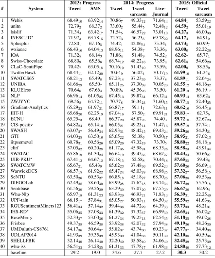
The results for subtask B are shown in Table 11. Again, we show results on the five progress test datasets from 2013 and 2014, in addition to those for the official Twitter2015-test datasets.
Subtask B attracted 40 teams, both newcomers and returning, similarly to 2013 and 2014. All managed to beat the baseline with the exception of one system for Twitter2015-test, and one for Twitter2014-test. There is a cluster of four teams at the top: Webis (ensemble combining four Twit-ter sentiment classification approaches that partici-pated in previous editions) with anF1of 64.84, unitn
with 64.59, lsislif (logistic regression with special weighting for positives and negatives) with 64.27, and INESC-ID (word embeddings) with 64.17.
The last column in the table shows the results for the 2015 sarcastic tweets. Note that, unlike in 2014, this time they were not collected separately and did not have a special #sarcasm tag; instead, they are a subset of 75 tweets from Twitter2015-test that were flagged as sarcastic by the human annotators. The top system is IOA with anF1of 65.77, followed by
INESC-ID with 64.91, and NLP with 63.62.
2013: Progress 2014: Progress 2015: Official
# System Tweet SMS Tweet Tweet Live- Tweet Tweet
sarcasm Journal sarcasm
1 Webis 68.4910 63.9214 70.867 49.3312 71.6414 64.841 53.5922
2 unitn 72.792 68.372 73.602 55.445 72.4812 64.592 55.0119
3 lsislif 71.344 63.4217 71.545 46.5722 73.0110 64.273 46.0033
4 INESC-ID? 71.97
3 63.7815 72.523 56.233 69.7822 64.174 64.912
5 Splusplus 72.801 67.165 74.421 42.8631 75.341 63.735 60.997
6 wxiaoac 66.4316 64.0413 68.9611 54.387 73.369 63.006 52.2226
7 IOA 71.325 68.143 71.864 51.489 74.522 62.627 65.771
8 Swiss-Chocolate 68.809 65.566 68.7412 48.2216 73.954 62.618 54.6620
9 CLaC-SentiPipe 70.427 63.0518 70.1610 51.4310 73.596 62.009 58.559
10 TwitterHawk 68.4411 62.1220 70.649 56.024 70.1719 61.9910 61.246
11 SWATCS65 68.2112 65.498 67.2314 37.2339 73.378 61.8911 52.6424
12 UNIBA 61.6629 65.507 65.1125 37.3038 70.0520 61.5512 48.1632
13 KLUEless 70.646 67.664 70.896 45.3626 73.507 61.2013 56.1917
14 NLP 66.9614 61.0525 67.4513 39.8734 66.1231 60.9314 63.623
15 ZWJYYC 69.568 64.7211 70.778 46.3423 71.6015 60.7715 52.4025
16 Gradiant-Analytics 65.2922 61.9721 66.8717 59.111 72.6311 60.6216 56.4516
17 IIIT-H 65.6820 62.2519 67.0416 57.502 69.9121 59.8317 62.755
18 ECNU 65.2523 68.491 66.3720 45.8725 74.403 59.7218 52.6723
19 CIS-positiv 64.8224 65.1410 66.0521 49.2314 71.4716 59.5719 57.7411
20 SWASH 63.0727 56.4934 62.9331 48.4215 69.4324 59.2620 54.3021
21 GTI 64.0325 63.5016 65.6522 55.386 70.5017 58.9521 57.0213
22 iitpsemeval 60.7831 60.5626 65.0926 47.3219 73.705 58.8022 58.1810
23 elirf 57.0532 60.2028 61.1735 45.9824 68.3328 58.5823 43.9134
24 SWATAC 65.8619 61.3024 66.6419 39.4535 68.6727 58.4324 50.6627
25 UIR-PKU? 67.41
13 64.6712 67.1815 52.588 70.4418 57.6525 59.438
26 SWATCMW 65.6721 65.439 65.6223 37.4836 69.5223 57.6026 56.6914
27 WarwickDCS 66.5715 61.9222 65.4724 45.0328 68.9825 57.3227 56.5815
28 SeNTU 63.5026 60.5327 66.8518 45.1827 68.7026 57.0628 49.5329
29 DIEGOLab 62.4928 58.6030 63.9928 47.6218 63.7434 56.7229 55.5618
30 Sentibase 61.5630 59.2629 63.2930 47.0720 67.5529 56.6730 62.964
31 Whu-Nlp 65.9718 61.3123 63.9329 46.9321 71.8313 56.3931 22.2540
32 UPF-taln 66.1517 57.8431 65.0527 50.9311 64.5032 55.5932 41.6335
33 RGUSentimentMiners123 56.4134 57.1432 59.4436 44.7229 64.3933 53.7333 48.2131
34 IHS-RD? 55.06
35 57.0833 61.3932 37.3237 66.9930 52.6534 36.0237
35 RoseMerry 52.3337 53.0036 61.2734 49.2513 62.5435 51.1835 49.6228
36 Frisbee 49.3738 46.5938 53.9238 42.0732 57.9438 49.1936 48.2630
37 UMDuluth-CS8761 54.1736 50.6437 55.8237 43.7430 60.2337 47.7737 34.4038
38 UDLAP2014 41.9339 39.3539 45.9339 41.0433 50.1139 42.1038 40.5936
39 SHELLFBK 32.1440 26.1440 32.2040 35.5840 34.0640 32.4539 25.7339
40 whu-iss 56.5133 54.2835 61.3133 47.7817 61.9836 24.8040 57.7312
[image:9.612.87.529.55.587.2]baseline 29.2 19.0 34.6 27.7 27.2 30.3 30.2
Table 11:Results for subtask B: Message-Level Polarity.The systems are ordered by their score on the Twitter2015 test dataset; the rankings on the individual datasets are indicated with a subscript. Systems with late submissions for
theprogresstest datasets (but with timely submissions for the official 2015 test dataset) are marked with a?.
Compared to 2014, there is improvement on Twitter2013-test from 72.12 (TeamX) to 72.80 (Splusplus), on Twitter2014-test from 70.96 (TeamX) to 74.42 (Spluplus), on
# System Tweet Tweet sarcasm 1 TwitterHawk 50.511 31.302
2 KLUEless 45.482 39.261
3 Whu-Nlp 40.703 23.375
4 whu-iss 25.624 28.904
5 ECNU 25.385 16.206
6 WarwickDCS 22.796 13.577
7 UMDuluth-CS8761 18.997 29.913
[image:10.612.87.284.54.176.2]baseline 26.7 26.4
Table 12:Results for Subtask C: Topic-Level Polarity. The systems are ordered by the official 2015 score.
# Team avgDiff avgLevelDiff
1 KLUEless 0.202 0.810
2 Whu-Nlp 0.210 0.869
3 TwitterHawk 0.214 0.978
4 whu-iss 0.256 1.007
5 ECNU 0.300 1.190
6 UMDuluth-CS8761 0.309 1.314
[image:10.612.75.293.219.319.2]baseline 0.277 0.985
Table 13: Results for Subtask D: Trend Towards a Topic.The systems are sorted by the official 2015 score.
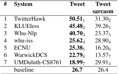
5.3 Subtask C: Topic-Level Polarity
The results for subtask C are shown in Table 12. This proved to be a hard subtask, and only three of the seven teams that participated in it managed to improve over a majority vote baseline. These three teams, TwitterHawk (using subtask B data to help with subtask C) withF1=50.51, KLUEless
(which ignored the topics as if it was subtask B) with F1=45.48, and Whu-Nlp with F1=40.70, achieved
scores that outperform the rest by a sizable margin: 15-25 points absolute more than the fourth team.
Note that, despite the apparent similarity, subtask C is much harder than subtask B: the top-3 teams achieved anF1 of 64-65 for subtask B vs. anF1 of
41-51 for subtask C. This cannot be blamed on the class distribution, as the difference in performance of the majority class baseline is much smaller: 30.3 for B vs. 26.7 for C.
Finally, the last column in the table reports the results for the 75 sarcastic 2015 tweets. The win-ner here is KLUEless with an F1 of 39.26,
fol-lowed by TwitterHawk withF1=31.30, and then by
UMDuluth-CS8761 withF1=29.91.
5.4 Subtask D: Trend Towards a Topic
The results for subtask D are shown in Table 13. This subtask is closely related to subtask C (in fact, one obvious way to solve D is to solve C and then to calculate the proportion), and thus it has attracted the same teams, except for one. Again, only three of the participating teams managed to improve over the baseline; not suprisingly, those were the same three teams that were in top-3 for subtask C. How-ever, the ranking is different from that in subtask C, e.g., TwitterHawk has dropped to third position, while KLUEless and Why-Nlp have each climbed one position up to positions 1 and 2, respectively.
Finally, note that avgDiff and avgLevelDiff yielded the same rankings.
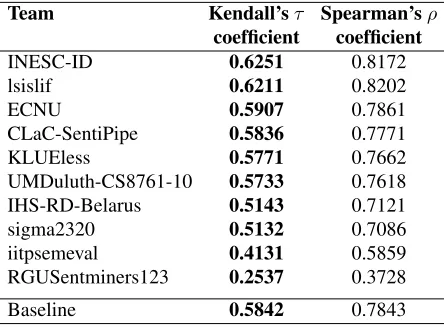
5.5 Subtask E: Degree of Prior Polarity
Ten teams participated in subtask E. Many chose an unsupervised approach and leveraged newly-created and pre-existing sentiment lexicons such as the Hashtag Sentiment Lexicon, the Sentiment140 Lexicon (Kiritchenko et al., 2014), the MPQA Sub-jectivity Lexicon (Wilson et al., 2005), and Sen-tiWordNet (Baccianella et al., 2010), among oth-ers. Several participants further automatically cre-ated their own sentiment lexicons from large collec-tions of tweets. Three teams, including the winner INESC-ID, adopted a supervised approach and used word embeddings (supplemented with lexicon fea-tures) to train a regression model.
The results are presented in Table 14. The last row shows the performance of a lexicon-based baseline. For this baseline, we chose the two most frequently used existing, publicly available, and automatically generated sentiment lexicons: Hashtag Sentiment Lexicon and Sentiment140 Lexicon (Kiritchenko et al., 2014).5 These lexicons have real-valued
senti-ment scores for most of the terms in the test set. For negated phrases, we use the scores of the cor-responding negated entries in the lexicons. For each term, we take its score from the Sentiment140 Lex-icon if present; otherwise, we take the term’s score from the Hashtag Sentiment Lexicon. For terms not found in any lexicon, we use the score of 0, which indicates a neutral term in these lexicons. The top three teams were able to improve over the baseline.
Team Kendall’sτ Spearman’sρ coefficient coefficient
INESC-ID 0.6251 0.8172
lsislif 0.6211 0.8202
ECNU 0.5907 0.7861
CLaC-SentiPipe 0.5836 0.7771
KLUEless 0.5771 0.7662
UMDuluth-CS8761-10 0.5733 0.7618 IHS-RD-Belarus 0.5143 0.7121
sigma2320 0.5132 0.7086
iitpsemeval 0.4131 0.5859
RGUSentminers123 0.2537 0.3728
[image:11.612.73.295.54.218.2]Baseline 0.5842 0.7843
Table 14: Results for Subtask E: Degree of Prior Po-larity. The systems are ordered by their Kendall’s τ
score, which was the official score.
6 Discussion
As in the previous two years, almost all systems used supervised learning. Popular machine learning ap-proaches included SVM, maximum entropy, CRFs, and linear regression. In several of the subtasks, the top system used deep neural networks and word em-beddings, and some systems benefited from special weighting of the positive and negative examples.
Once again, the most important features were those derived from sentiment lexicons. Other impor-tant features included bag-of-words features, hash-tags, handling of negation, word shape and punctua-tion features, elongated words, etc. Moreover, tweet pre-processing and normalization were an important part of the processing pipeline.
Note that this year we did not make a distinc-tion between constrained and unconstrained sys-tems, and participants were free to use any addi-tional data, resources and tools they wished to.
Overall, the task has attracted a total of 41 teams, which is comparable to previous editions: there were 46 teams in 2014, and 44 in 2013. As in previous years, subtask B was most popular, attracting almost all teams (40 out of 41). However, subtask A at-tracted just a quarter of the participants (11 out of 41), compared to about half in previous years, most likely due to the introduction of two new, very re-lated subtasks C and D (with 6 and 7 participants, respectively). There was also a fifth subtask (E, with 10 participants), which further contributed to the participant split.
We should further note that our task was part of a larger Sentiment Track, together with three other closely-related tasks, which were also interested in sentiment analysis: Task 9 on CLIPEval Implicit Po-larity of Events, Task 11 on Sentiment Analysis of Figurative Language in Twitter, and Task 12 on As-pect Based Sentiment Analysis. Another related task was Task 1 on Paraphrase and Semantic Similarity in Twitter, from the Text Similarity and Question An-swering track, which also focused on tweets.
7 Conclusion
We have described the five subtasks organized as part of SemEval-2015 Task 10 on Sentiment Anal-ysis in Twitter: detecting sentiment of terms in con-text (subtask A), classifiying the sentiment of an entire tweet, SMS message or blog post (subtask B), predicting polarity towards a topic (subtask C), quantifying polarity towards a topic (subtask D), and proposing real-valued prior sentiment scores for Twitter terms (subtask E). Over 40 teams partici-pated in these subtasks, using various techniques.
We plan a new edition of the task as part of SemEval-2016, where we will focus on sentiment with respect to a topic, but this time on a five-point scale, which is used for human review ratings on popular websites such as Amazon, TripAdvisor, Yelp, etc. From a research perspective, moving to an ordered five-point scale means moving from binary classification toordinal regression.
We further plan to continue the trend detection subtask, which represents a move from classification toquantification, and is on par with what applica-tions need. They are not interested in the sentiment of a particular tweet but rather in the percentage of tweets that are positive/negative.
Finally, we plan a new subtask on trend detection, but using a five-point scale, which would get us even closer to what business (e.g. marketing studies), and researchers, (e.g. in political science or public pol-icy), want nowadays. From a research perspective, this is a problem ofordinal quantification.
Acknowledgements
References
Eric Almquist and Jason Lee. 2009. What do customers really want? Harvard Business Review.
Stefano Baccianella, Andrea Esuli, and Fabrizio Sebas-tiani. 2010. SentiWordNet 3.0: An enhanced lexical resource for sentiment analysis and opinion mining. In
Proceedings of the Seventh International Conference
on Language Resources and Evaluation, LREC ’10,
pages 2200–2204, Valletta, Malta.
Luciano Barbosa and Junlan Feng. 2010. Robust senti-ment detection on Twitter from biased and noisy data.
In Proceedings of the 23rd International Conference
on Computational Linguistics: Posters, COLING ’10,
pages 36–44, Beijing, China.
Albert Bifet, Geoffrey Holmes, Bernhard Pfahringer, and Ricard Gavald`a. 2011. Detecting sentiment change in Twitter streaming data. Journal of Machine Learning
Research, Proceedings Track, 17:5–11.
Dmitry Davidov, Oren Tsur, and Ari Rappoport. 2010. Semi-supervised recognition of sarcasm in Twitter and Amazon. In Proceedings of the Fourteenth
Confer-ence on Computational Natural Language Learning,
CoNLL ’10, pages 107–116, Uppsala, Sweden. Roberto Gonz´alez-Ib´a˜nez, Smaranda Muresan, and Nina
Wacholder. 2011. Identifying sarcasm in Twitter: a closer look. InProceedings of the 49th Annual Meet-ing of the Association for Computational LMeet-inguistics:
Human Language Technologies - Short Papers,
ACL-HLT ’11, pages 581–586, Portland, Oregon, USA. Dustin Hillard, Mari Ostendorf, and Elizabeth Shriberg.
2003. Detection of agreement vs. disagreement in meetings: Training with unlabeled data. In Proceed-ings of the 2003 Conference of the North American Chapter of the Association for Computational
Lin-guistics on Human Language Technology: Volume 2,
NAACL ’03, pages 34–36, Edmonton, Canada. Minqing Hu and Bing Liu. 2004. Mining and
summa-rizing customer reviews. In Proceedings of the 10th ACM SIGKDD International Conference on
Knowl-edge Discovery and Data Mining, KDD ’04, pages
168–177, New York, NY, USA.
Bernard Jansen, Mimi Zhang, Kate Sobel, and Abdur Chowdury. 2009. Twitter power: Tweets as elec-tronic word of mouth. J. Am. Soc. Inf. Sci. Technol., 60(11):2169–2188.
David Jurgens, Saif Mohammad, Peter Turney, and Keith Holyoak. 2012. SemEval-2012 Task 2: Measuring degrees of relational similarity. InProceedings of the
Sixth International Workshop on Semantic Evaluation,
SemEval ’12, pages 356–364, Montr´eal, Canada. Maurice G Kendall. 1938. A new measure of rank
corre-lation. Biometrika, pages 81–93.
Svetlana Kiritchenko, Xiaodan Zhu, and Saif M. Mo-hammad. 2014. Sentiment analysis of short infor-mal texts. Journal of Artificial Intelligence Research
(JAIR), 50:723–762.
Efthymios Kouloumpis, Theresa Wilson, and Johanna Moore. 2011. Twitter sentiment analysis: The good the bad and the OMG! In Proceedings of the Fifth International Conference on Weblogs and Social Me-dia, ICWSM ’11, pages 538–541, Barcelona, Catalo-nia, Spain.
Erich Leo Lehmann and Howard JM D’Abrera. 2006.
Nonparametrics: statistical methods based on ranks.
Springer New York.
Christine Liebrecht, Florian Kunneman, and Antal Van den Bosch. 2013. The perfect solution for de-tecting sarcasm in tweets #not. InProceedings of the 4th Workshop on Computational Approaches to
Sub-jectivity, Sentiment and Social Media Analysis, pages
29–37, Atlanta, Georgia, USA.
Jordan J. Louviere. 1991. Best-worst scaling: A model for the largest difference judgments. Technical report, University of Alberta.
Saif Mohammad, Svetlana Kiritchenko, and Xiaodan Zhu. 2013. NRC-Canada: Building the state-of-the-art in sentiment analysis of tweets. InProceedings of the Seventh International Workshop on Semantic
Eval-uation, SemEval ’13, pages 321–327, Atlanta,
Geor-gia, USA.
Preslav Nakov, Sara Rosenthal, Zornitsa Kozareva, Veselin Stoyanov, Alan Ritter, and Theresa Wilson. 2013. SemEval-2013 Task 2: Sentiment analysis in Twitter. In Proceedings of the Seventh
Interna-tional Workshop on Semantic Evaluation, SemEval
’13, pages 312–320, Atlanta, Georgia, USA.
Brendan O’Connor, Ramnath Balasubramanyan, Bryan Routledge, and Noah Smith. 2010. From tweets to polls: Linking text sentiment to public opinion time se-ries. InProceedings of the Fourth International
Con-ference on Weblogs and Social Media, ICWSM ’10,
pages 122–129, Washington, DC, USA.
Alexander Pak and Patrick Paroubek. 2010. Twitter based system: Using Twitter for disambiguating senti-ment ambiguous adjectives. InProceedings of the 5th
International Workshop on Semantic Evaluation,
Se-mEval ’10, pages 436–439, Uppsala, Sweden. Bo Pang, Lillian Lee, and Shivakumar Vaithyanathan.
2002. Thumbs up?: Sentiment classification using ma-chine learning techniques. InProceedings of the Con-ference on Empirical Methods in Natural Language
Processing - Volume 10, EMNLP ’02, pages 79–86,
Philadephia, Pennsylvania, USA.
Proceedings of the Conference on Empirical Methods
in Natural Language Processing, EMNLP ’11, pages
1524–1534, Edinburgh, Scotland, UK.
Alan Ritter, Oren Etzioni, Sam Clark, et al. 2012. Open domain event extraction from Twitter. InProceedings of the 18th ACM SIGKDD International Conference
on Knowledge Discovery and Data Mining, KDD ’12,
pages 1104–1112, Beijing, China.
Sara Rosenthal, Alan Ritter, Preslav Nakov, and Veselin Stoyanov. 2014. SemEval-2014 Task 9: Sentiment analysis in Twitter. In Proceedings of the 8th
In-ternational Workshop on Semantic Evaluation,
Se-mEval ’14, pages 73–80, Dublin, Ireland.
Janyce Wiebe, Theresa Wilson, and Claire Cardie. 2005. Annotating expressions of opinions and emotions in language. Language Resources and Evaluation, 39(2-3):165–210.
Theresa Wilson, Janyce Wiebe, and Paul Hoffmann. 2005. Recognizing contextual polarity in phrase-level sentiment analysis. InProceedings of the Con-ference on Human Language Technology and
Em-pirical Methods in Natural Language Processing,
HLT-EMNLP ’05, pages 347–354, Vancouver, British Columbia, Canada.
Xiaodan Zhu, Hongyu Guo, Saif Mohammad, and Svet-lana Kiritchenko. 2014. An empirical study on the effect of negation words on sentiment. In Proceed-ings of the 52nd Annual Meeting of the Association for
Computational Linguistics (Volume 1: Long Papers),