Bayesian Inference for PCFGs via Markov chain Monte Carlo
Mark Johnson
Cognitive and Linguistic Sciences Brown University
Mark [email protected]
Thomas L. Griffiths Department of Psychology University of California, Berkeley
Sharon Goldwater Department of Linguistics
Stanford University
Abstract
This paper presents two Markov chain Monte Carlo (MCMC) algorithms for Bayesian inference of probabilistic con-text free grammars (PCFGs) from ter-minal strings, providing an alternative to maximum-likelihood estimation using the Inside-Outside algorithm. We illus-trate these methods by estimating a sparse grammar describing the morphology of the Bantu language Sesotho, demonstrat-ing that with suitable priors Bayesian techniques can infer linguistic structure in situations where maximum likelihood methods such as the Inside-Outside algo-rithm only produce a trivial grammar.
1 Introduction
The standard methods for inferring the parameters of probabilistic models in computational linguistics are based on the principle of maximum-likelihood esti-mation; for example, the parameters of Probabilistic Context-Free Grammars (PCFGs) are typically es-timated from strings of terminals using the Inside-Outside (IO) algorithm, an instance of the Ex-pectation Maximization (EM) procedure (Lari and Young, 1990). However, much recent work in ma-chine learning and statistics has turned away from maximum-likelihood in favor of Bayesian methods, and there is increasing interest in Bayesian methods in computational linguistics as well (Finkel et al., 2006). This paper presents two Markov chain Monte
Carlo (MCMC) algorithms for inferring PCFGs and their parses from strings alone. These can be viewed as Bayesian alternatives to the IO algorithm.
The goal of Bayesian inference is to compute a distribution over plausible parameter values. This “posterior” distribution is obtained by combining the likelihood with a “prior” distribution P(θ) over pa-rameter valuesθ. In the case of PCFG inferenceθis the vector of rule probabilities, and the prior might assert a preference for a sparse grammar (see be-low). The posterior probability of each value of θ
is given by Bayes’ rule:
P(θ|D) ∝ P(D|θ)P(θ). (1)
In principle Equation 1 defines the posterior prob-ability of any value of θ, but computing this may not be tractable analytically or numerically. For this reason a variety of methods have been developed to support approximate Bayesian inference. One of the most popular methods is Markov chain Monte Carlo (MCMC), in which a Markov chain is used to sam-ple from the posterior distribution.
This paper presents two new MCMC algorithms for inferring the posterior distribution over parses and rule probabilities given a corpus of strings. The first algorithm is a component-wise Gibbs sampler which is very similar in spirit to the EM algo-rithm, drawing parse trees conditioned on the cur-rent parameter values and then sampling the param-eters conditioned on the current set of parse trees. The second algorithm is a component-wise Hastings sampler that “collapses” the probabilistic model, in-tegrating over the rule probabilities of the PCFG, with the goal of speeding convergence. Both
rithms use an efficient dynamic programming tech-nique to sample parse trees.
Given their usefulness in other disciplines, we believe that Bayesian methods like these are likely to be of general utility in computational linguis-tics as well. As a simple illustrative example, we use these methods to infer morphological parses for verbs from Sesotho, a southern Bantu language with agglutinating morphology. Our results illustrate that Bayesian inference using a prior that favors sparsity can produce linguistically reasonable analyses in sit-uations in which EM does not.
The rest of this paper is structured as follows. The next section introduces the background for our paper, summarizing the key ideas behind PCFGs, Bayesian inference, and MCMC. Section 3 intro-duces our first MCMC algorithm, a Gibbs sampler for PCFGs. Section 4 describes an algorithm for sampling trees from the distribution over trees de-fined by a PCFG. Section 5 shows how to integrate out the rule weight parameters θin a PCFG, allow-ing us to sample directly from the posterior distribu-tion over parses for a corpus of strings. Finally, Sec-tion 6 illustrates these methods in learning Sesotho morphology.
2 Background
2.1 Probabilistic context-free grammars
LetG = (T, N, S, R) be a Context-Free Grammar in Chomsky normal form with no useless produc-tions, whereT is a finite set of terminal symbols,N
is a finite set of nonterminal symbols (disjoint from
T),S∈N is a distinguished nonterminal called the
start symbol, andRis a finite set of productions of the formA→B CorA→w, whereA, B, C ∈N
andw ∈T. In what follows we useβ as a variable ranging over(N ×N)∪T.
A Probabilistic Context-Free Grammar(G, θ)is a pair consisting of a context-free grammar G and a real-valued vectorθof length|R|indexed by pro-ductions, whereθA→β is the production probability associated with the production A → β ∈ R. We require thatθA→β ≥0and that for all nonterminals A∈N,P
A→β∈RθA→β = 1.
A PCFG(G, θ)defines a probability distribution
over treestas follows:
PG(t|θ) =
Y
r∈R θfr(t)
r
wheretis generated by Gand fr(t) is the number of times the production r = A → β ∈ R is used in the derivation oft. IfG does not generate t let PG(t|θ) = 0. The yield y(t) of a parse tree t is the sequence of terminals labeling its leaves. The probability of a string w ∈ T+ of terminals is the sum of the probability of all trees with yieldw, i.e.:
PG(w|θ) =
X
t:y(t)=w
PG(t|θ).
2.2 Bayesian inference for PCFGs
Given a corpus of stringsw= (w1, . . . , wn), where
eachwiis a string of terminals generated by a known CFGG, we would like to be able to infer the pro-duction probabilitiesθthat best describe that corpus. Takingwto be our data, we can apply Bayes’ rule
(Equation 1) to obtain:
P(θ|w) ∝ PG(w|θ)P(θ), where PG(w|θ) =
n
Y
i=1
PG(wi|θ).
Usingt to denote a sequence of parse trees for w,
we can compute the joint posterior distribution over
tandθ, and then marginalize overt, withP(θ|w) =
P
tP(t, θ|w). The joint posterior distribution on t
andθis given by:
P(t, θ|w) ∝ P(w|t)P(t|θ)P(θ) =
n
Y
i=1
P(wi|ti)P(ti|θ)
!
P(θ)
withP(wi|ti) = 1ify(ti) =wi, and0otherwise.
2.3 Dirichlet priors
The first step towards computing the posterior dis-tribution is to define a prior on θ. We takeP(θ)to be a product of Dirichlet distributions, with one dis-tribution for each non-terminal A ∈ N. The prior is parameterized by a positive real valued vector α
with left-hand side A, and let θA and αA refer to the component subvectors of θ and α respectively indexed by productions in RA. The Dirichlet prior PD(θ|α)is:
PD(θ|α) =
Y
A∈N
PD(θA|αA), where
PD(θA|αA) = 1 C(αA)
Y
r∈RA
θαr−1
r and
C(αA) =
Q
r∈RAΓ(αr)
Γ(P
r∈RAαr)
(2)
where Γ is the generalized factorial function and
C(α) is a normalization constant that does not de-pend onθA.
Dirichlet priors are useful because they are
con-jugate to the distribution over trees defined by a
PCFG. This means that the posterior distribution on θgiven a set of parse trees, P(θ|t, α), is also a
Dirichlet distribution. Applying Bayes’ rule,
PG(θ|t, α) ∝ PG(t|θ) PD(θ|α)
∝ Y
r∈R θfr(t)
r
! Y
r∈R θαr−1
r
!
= Y
r∈R
θfr(t)+αr−1
r
which is a Dirichlet distribution with parameters
f(t) + α, where f(t) is the vector of production
counts intindexed byr∈R. We can thus write: PG(θ|t, α) = PD(θ|f(t) +α)
which makes it clear that the production counts com-bine directly with the parameters of the prior.
2.4 Markov chain Monte Carlo
Having defined a prior onθ, the posterior distribu-tion over t and θ is fully determined by a corpus w. Unfortunately, computing the posterior
probabil-ity of even a single choice oftandθis intractable,
as evaluating the normalizing constant for this dis-tribution requires summing over all possible parses for the entire corpus and all sets of production prob-abilities. Nonetheless, it is possible to define al-gorithms that sample from this distribution using Markov chain Monte Carlo (MCMC).
MCMC algorithms construct a Markov chain whose statess∈ S are the objects we wish to sam-ple. The state space S is typically astronomically
large — in our case, the state space includes all pos-sible parses of the entire training corpus w— and
the transition probabilitiesP(s′
|s)are specified via a scheme guaranteed to converge to the desired distri-butionπ(s)(in our case, the posterior distribution). We “run” the Markov chain (i.e., starting in initial states0, sample a states1 fromP(s′|s0), then sam-ple states2fromP(s′|s1), and so on), with the prob-ability that the Markov chain is in a particular state, P(si), converging toπ(si)asi→ ∞.
After the chain has run long enough for it to ap-proach its stationary distribution, the expectation Eπ[f] of any function f(s) of the state s will be approximated by the average of that function over the set of sample states produced by the algorithm. For example, in our case, given samples(ti, θi)for i= 1, . . . , ℓproduced by an MCMC algorithm, we can estimateθas
Eπ[θ] ≈ 1 ℓ
ℓ
X
i=1 θi
The remainder of this paper presents two MCMC algorithms for PCFGs. Both algorithms proceed by setting the initial state of the Markov chain to a guess for(t, θ)and then sampling successive states using
a particular transition matrix. The key difference be-twen the two algorithms is the form of the transition matrix they assume.
3 A Gibbs sampler forP(t, θ|w, α)
The Gibbs sampler (Geman and Geman, 1984) is one of the simplest MCMC methods, in which tran-sitions between states of the Markov chain result from sampling each component of the state condi-tioned on the current value of all other variables. In our case, this means alternating between sampling from two distributions:
P(t|θ,w, α) = n
Y
i=1
P(ti|wi, θ), and
P(θ|t,w, α) = PD(θ|f(t) +α)
= Y
A∈N
PD(θA|fA(t) +αA).
Thus every two steps we generate a new sample of
t and θ. This alternation between parsing and
ti
t1 tn
w1 wi wn
θAj
. . .
θA1 . . . θA|N|
αA1 . . . αAj . . . αA|N|
. . . . . . . . .
[image:4.612.100.272.58.161.2]. . .
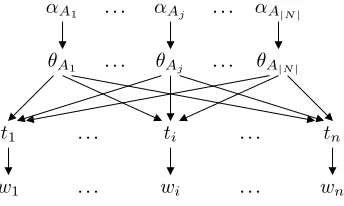
Figure 1: A Bayes net representation of dependen-cies among the variables in a PCFG.
the Expectation step replaced by samplingtand the
Maximization step replaced by samplingθ.
The dependencies among variables in a PCFG are depicted graphically in Figure 1, which makes clear that the Gibbs sampler is highly parallelizable (just like the EM algorithm). Specifically, the parses ti are independent given θ and so can be sampled in parallel from the following distribution as described in the next section.
PG(ti|wi, θ) =
PG(ti|θ) PG(wi|θ)
We make use of the fact that the posterior is a product of independent Dirichlet distributions in or-der to sample θ from PD(θ|t, α). The production probabilities θA for each nonterminal A ∈ N are sampled from a Dirchlet distibution with parameters
α′
A = fA(t) +αA. There are several methods for samplingθ = (θ1, . . . , θm)from a Dirichlet distri-bution with parameters α= (α1, . . . , αm), with the simplest being samplingxj from a Gamma(αj) dis-tribution for j = 1, . . . , m and then setting θj = xj/Pmk=1xk(Gentle, 2003).
4 Efficiently sampling fromP(t|w, θ)
This section completes the description of the Gibbs sampler for(t, θ)by describing a dynamic
program-ming algorithm for sampling trees from the set of parses for a string generated by a PCFG. This al-gorithm appears fairly widely known: it was de-scribed by Goodman (1998) and Finkel et al (2006) and used by Ding et al (2005), and is very simi-lar to other dynamic programming algorithms for CFGs, so we only summarize it here. The algo-rithm consists of two steps. The first step con-structs a standard “inside” table or chart, as used in
the Inside-Outside algorithm for PCFGs (Lari and Young, 1990). The second step involves a recursion from larger to smaller strings, sampling from the productions that expand each string and construct-ing the correspondconstruct-ing tree in a top-down fashion.
In this section we takewto be a string of terminal symbols w = (w1, . . . , wn) where each wi ∈ T, and define wi,k = (wi+1, . . . , wk) (i.e., the sub-string from wi+1 up to wk). Further, let GA = (T, N, A, R), i.e., a CFG just likeGexcept that the start symbol has been replaced withA, so,PGA(t|θ)
is the probability of a tree twhose root node is la-beledAand PGA(w|θ)is the sum of the
probabili-ties of all trees whose root nodes are labeledAwith yieldw.
The Inside algorithm takes as input a PCFG (G, θ) and a string w = w0,n and constructs a ta-ble with entries pA,i,k for each A ∈ N and 0 ≤ i < k ≤ n, wherepA,i,k = PGA(wi,k|θ), i.e., the
probability ofArewriting towi,k. The table entries are recursively defined below, and computed by enu-merating all feasiblei, kandAin any order such that all smaller values ofk−iare enumerated before any larger values.
pA,k−1,k = θA→wk
pA,i,k =
X
A→B C∈R
X
i<j<k
θA→B CpB,i,j pC,j,k
for allA, B, C ∈N and0≤i < j < k≤n. At the end of the Inside algorithm,PG(w|θ) =pS,0,n.
The second step of the sampling algorithm uses the function SAMPLE, which returns a sample from
PG(t|w, θ) given the PCFG (G, θ) and the inside table pA,i,k. SAMPLE takes as arguments a non-terminal A ∈ N and a pair of string positions 0 ≤ i < k ≤ n and returns a tree drawn from PGA(t|wi,k, θ). It functions in a top-down fashion,
selecting the productionA→B Cto expand theA, and then recursively calling itself to expand B and
Crespectively.
function SAMPLE(A, i, k) :
ifk−i= 1then return TREE(A, wk)
(j, B, C) =MULTI(A, i, k)
return TREE(A,SAMPLE(B, i, j),SAMPLE(C, j, k))
MULTI is a function that produces samples from a multinomial distribution over the possible “split” positions j and nonterminal children B and C, where:
P(j, B, C) = θA→B CPGB(wi,j|θ) PGC(wj,k|θ)
PGA(wi,k|θ)
5 A Hastings sampler forP(t|w, α)
The Gibbs sampler described in Section 3 has the disadvantage that each sample of θ re-quires reparsing the training corpus w. In
this section, we describe a component-wise Hastings algorithm for sampling directly from P(t|w, α), marginalizing over the
produc-tion probabilities θ. Transitions between states are produced by sampling parses ti from P(ti|wi,t−i, α) for each string wi in turn, where t−i = (t1, . . . , ti−1, ti+1, . . . , tn) is the current set
of parses forw−i = (w1, . . . , wi−1, wi+1, . . . , wn).
Marginalizing over θ effectively means that the production probabilities are updated after each sentence is parsed, so it is reasonable to expect that this algorithm will converge faster than the Gibbs sampler described earlier. While the sampler does not explicitly provide samples ofθ, the results outlined in Sections 2.3 and 3 can be used to sample the posterior distribution overθ for each sample of
tif required.
LetPD(θ|α)be a Dirichlet product prior, and let ∆be the probability simplex for θ. Then by inte-grating over the posterior Dirichlet distributions we have:
P(t|α) =
Z
∆
PG(t|θ)PD(θ|α)dθ
= Y
A∈N
C(αA+fA(t)) C(αA)
(3)
where C was defined in Equation 2. Because we are marginalizing overθ, the treestibecome depen-dent upon one another. Intuitively, this is because
wimay provide information about θthat influences how some other stringwj should be parsed.
We can use Equation 3 to compute the conditional probabilityP(ti|t−i, α)as follows:
P(ti|t−i, α) =
P(t|α) P(t−i|α)
= Y
A∈N
C(αA+fA(t)) C(αA+fA(t−i)) Now, if we could sample from
P(ti|wi,t−i, α) =
P(wi|ti)P(ti|t−i, α)
P(wi|t−i, α)
we could construct a Gibbs sampler whose states were the parse treest. Unfortunately, we don’t even
know if there is an efficient algorithm for calculat-ingP(wi|t−i, α), let alone an efficient sampling al-gorithm for this distribution.
Fortunately, this difficulty is not fatal. A Hast-ings sampler for a probability distribution π(s) is an MCMC algorithm that makes use of a proposal
distribution Q(s′|s) from which it draws samples,
and uses an acceptance/rejection scheme to define a transition kernel with the desired distribution π(s). Specifically, given the current states, a samples′6= sdrawn from Q(s′|s) is accepted as the next state
with probability
A(s, s′
) = min
1,π(s
′)Q(s|s′) π(s)Q(s′|s)
and with probability1−A(s, s′)
the proposal is re-jected and the next state is the current states.
We use a component-wise proposal distribution, generating new proposed values for ti, where i is chosen at random. Our proposal distribution is the posterior distribution over parse trees generated by the PCFG with grammar G and production proba-bilities θ′
, where θ′
is chosen based on the current
t−i as described below. Each step of our Hastings
sampler is as follows. First, we compute θ′
from
t−i as described below. Then we sample t′
i from P(ti|wi, θ′) using the algorithm described in Sec-tion 4. Finally, we accept the proposal t′
i given the old parsetiforwi with probability:
A(ti, t′i) = min
(
1,P(t ′
i|wi,t−i, α)P(ti|wi, θ′) P(ti|wi,t−i, α)P(t
′
i|wi, θ′)
)
= min
(
1,P(t ′
i|t−i, α)P(ti|wi, θ′) P(ti|t−i, α)P(t′i|wi, θ′)
)
compute P(wi|t−i, α) is a common factor of both the numerator and denominator, and hence is not re-quired. TheP(wi|ti)term also disappears, being 1 for both the numerator and the denominator since our proposal distribution can only generate trees for whichwiis the yield.
All that remains is to specify the production prob-abilities θ′ of the proposal distributionP(t′
i|wi, θ′). While the acceptance rule used in the Hastings algorithm ensures that it produces samples from P(ti|wi,t−i, α) with any proposal grammar θ′ in which all productions have nonzero probability, the algorithm is more efficient (i.e., fewer proposals are rejected) if the proposal distribution is close to the distribution to be sampled.
Given the observations above about the corre-spondence between terms in P(ti|t−i, α) and the relative frequency of the corresponding productions int−i, we setθ′
to the expected valueE[θ|t−i, α]of θgivent−iandαas follows:
θ′
r =
fr(t−i) +αr
P
r′∈RAfr′(t−i) +αr′
6 Inferring sparse grammars
As stated in the introduction, the primary contribu-tion of this paper is introducing MCMC methods for Bayesian inference to computational linguistics. Bayesian inference using MCMC is a technique of generic utility, much like Expectation-Maximization and other general inference techniques, and we be-lieve that it belongs in every computational linguist’s toolbox alongside these other techniques.
Inferring a PCFG to describe the syntac-tic structure of a natural language is an obvi-ous application of grammar inference techniques, and it is well-known that PCFG inference us-ing maximum-likelihood techniques such as the Inside-Outside (IO) algorithm, a dynamic program-ming Expectation-Maximization (EM) algorithm for PCFGs, performs extremely poorly on such tasks. We have applied the Bayesian MCMC methods de-scribed here to such problems and obtain results very similar to those produced using IO. We be-lieve that the primary reason why both IO and the Bayesian methods perform so poorly on this task is that simple PCFGs are not accurate models of English syntactic structure. We know that PCFGs
α= (0.1,1.0)
α= (0.5,1.0)
α= (1.0,1.0)
Binomial parameterθ1
P(θ1|α)
1 0.8 0.6 0.4 0.2 0
5
4
3
2
1
[image:6.612.315.521.56.169.2]0
Figure 2: A Dirichlet priorαon a binomial parame-terθ1. Asα1 →0,P(θ1|α)is increasingly concen-trated around0.
that represent only major phrasal categories ignore a wide variety of lexical and syntactic dependen-cies in natural language. State-of-the-art systems for unsupervised syntactic structure induction sys-tem uses models that are very different to these kinds of PCFGs (Klein and Manning, 2004; Smith and Eisner, 2006).1
Our goal in this section is modest: we aim merely to provide an illustrative example of Bayesian infer-ence using MCMC. As Figure 2 shows, when the Dirichlet prior parameter αr approaches 0 the prior probabilityPD(θr|α)becomes increasingly concen-trated around 0. This ability to bias the sampler toward sparse grammars (i.e., grammars in which many productions have probabilities close to 0) is useful when we attempt to identify relevant produc-tions from a much larger set of possible producproduc-tions via parameter estimation.
The Bantu language Sesotho is a richly agglutina-tive language, in which verbs consist of a sequence of morphemes, including optional Subject Markers (SM), Tense (T), Object Markers (OM), Mood (M)
and derivational affixes as well as the obligatory Verb stem (V), as shown in the following example:
re
SM
-a
T
-di
OM
-bon
V
-a
M
“We see them”
1
We used an implementation of the Hastings sampler described in Section 5 to infer morphological parses
t for a corpus w of 2,283 unsegmented Sesotho
verb types extracted from the Sesotho corpus avail-able from CHILDES(MacWhinney and Snow, 1985;
Demuth, 1992). We chose this corpus because the words have been morphologically segmented manu-ally, making it possible for us to evaluate the mor-phological parses produced by our system. We con-structed a CFGGcontaining the following produc-tions
Word → V
Word → V M
Word → SM V M
Word → SM T V M
Word → SM T OM V M
together with productions expanding the pretermi-nalsSM,T,OM,VandMto each of the 16,350 dis-tinct substrings occuring anywhere in the corpus, producting a grammar with 81,755 productions in all. In effect, G encodes the basic morphologi-cal structure of the Sesotho verb (ignoring factors such as derivation morphology and irregular forms), but provides no information about the phonological identity of the morphemes.
Note that Gactually generates a finite language. However, Gparameterizes the probability distribu-tion over the strings it generates in a manner that would be difficult to succintly characterize except in terms of the productions given above. Moreover, with approximately 20 times more productions than training strings, each string is highly ambiguous and estimation is highly underconstrained, so it provides an excellent test-bed for sparse priors.
We estimated the morphological parses t in two
ways. First, we ran the IO algorithm initialized with a uniform initial estimate θ0 forθ to produce an estimate of the MLE θˆ, and then computed the Viterbi parsesˆtof the training corpuswwith respect
to the PCFG(G,θˆ). Second, we ran the Hastings sampler initialized with trees sampled from(G, θ0) with several different values for the parameters of the prior. We experimented with a number of tech-niques for speeding convergence of both the IO and Hastings algorithms, and two of these were particu-larly effective on this problem. Annealing, i.e., us-ingP(t|w)1/τ in place ofP(t|w)whereτ is a
“tem-perature” parameter starting around 5 and slowly
ad-justed toward 1, sped the convergence of both algo-rithms. We ran both algorithms for several thousand iterations over the corpus, and both seemed to con-verge fairly quickly onceτ was set to 1. “Jittering” the initial estimate ofθused in the IO algorithm also sped its convergence.
The IO algorithm converges to a solution where
θWord→V = 1, and every stringw∈wis analysed
as a single morphemeV. (In fact, in this grammar P(wi|θ)is the empirical probability of wi, and it is easy to prove that thisθis the MLE).
The samples t produced by the Hastings
algo-rithm depend on the parameters of the Dirichlet prior. We set αr to a single value α for all pro-ductions r. We found that forα > 10−2 the sam-ples produced by the Hastings algorithm were the same trivial analyses as those produced by the IO algorithm, but as α was reduced below this t
be-gan to exhibit nontrivial structure. We evaluated the quality of the segmentations in the morpholog-ical analyses t in terms of unlabeled precision,
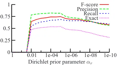
re-call, f-score and exact match (the fraction of words correctly segmented into morphemes; we ignored morpheme labels because the manual morphological analyses contain many morpheme labels that we did not include in G). Figure 3 contains a plot of how these quantities vary withα; obtaining an f-score of 0.75 and an exact word match accuracy of 0.54 at
α= 10−5(the corresponding values for the MLEθˆ are both 0). Note that we obtained good results asα
was varied over several orders of magnitude, so the actual value ofαis not critical. Thus in this appli-cation the ability to prefer sparse grammars enables us to find linguistically meaningful analyses. This ability to find linguistically meaningful structure is relatively rare in our experience with unsupervised PCFG induction.
We also experimented with a version of IO modi-fied to perform Bayesian MAP estimation, where the Maximization step of the IO procedure is replaced with Bayesian inference using a Dirichlet prior, i.e., where the rule probabilitiesθ(k)at iterationkare es-timated using:
Exact Recall PrecisionF-score
Dirichlet prior parameterαr
1 0.01 1e-04 1e-06 1e-08 1e-10 1
0.75
0.5
0.25
[image:8.612.86.292.55.168.2]0
Figure 3: Accuracy of morphological segmentations of Sesotho verbs proposed by the Hastings algo-rithms as a function of Dirichlet prior parameter
α. F-score, precision and recall are unlabeled mor-pheme scores, while Exact is the fraction of words correctly segmented.
and in some circumstances this may be a useful estimator. However, in our experiments with the Sesotho data above we found that for the small val-ues of α necessary to obtain a sparse solution,the expected rule countE[fr]for many rulesr was less than1−α. Thus on the next iterationθr= 0, result-ing in there beresult-ing no parse whatsoever for many of the strings in the training data. Variational Bayesian techniques offer a systematic way of dealing with these problems, but we leave this for further work.
7 Conclusion
This paper has described basic algorithms for per-forming Bayesian inference over PCFGs given ter-minal strings. We presented two Markov chain Monte Carlo algorithms (a Gibbs and a Hastings sampling algorithm) for sampling from the posterior distribution over parse trees given a corpus of their yields and a Dirichlet product prior over the produc-tion probabilities. As a component of these algo-rithms we described an efficient dynamic program-ming algorithm for sampling trees from a PCFG which is useful in its own right. We used these sampling algorithms to infer morphological analy-ses of Sesotho verbs given their strings (a task on which the standard Maximum Likelihood estimator returns a trivial and linguistically uninteresting so-lution), achieving 0.75 unlabeled morpheme f-score and 0.54 exact word match accuracy. Thus this is one of the few cases we are aware of in which a PCFG estimation procedure returns linguistically
meaningful structure. We attribute this to the ability of the Bayesian prior to prefer sparse grammars.
We expect that these algorithms will be of inter-est to the computational linguistics community both because a Bayesian approach to PCFG estimation is more flexible than the Maximum Likelihood meth-ods that currently dominate the field (c.f., the use of a prior as a bias towards sparse solutions), and because these techniques provide essential building blocks for more complex models.
References
Katherine Demuth. 1992. Acquisition of Sesotho. In Dan Slobin, editor, The Cross-Linguistic Study of Language
Ac-quisition, volume 3, pages 557–638. Lawrence Erlbaum
As-sociates, Hillsdale, N.J.
Ye Ding, Chi Yu Chan, and Charles E. Lawrence. 2005. RNA secondary structure prediction by centroids in a Boltzmann weighted ensemble. RNA, 11:1157–1166.
Jenny Rose Finkel, Christopher D. Manning, and Andrew Y. Ng. 2006. Solving the problem of cascading errors: Approximate Bayesian inference for linguistic annotation pipelines. In Proceedings of the 2006 Conference on
Empir-ical Methods in Natural Language Processing, pages 618–
626, Sydney, Australia. Association for Computational Lin-guistics.
Stuart Geman and Donald Geman. 1984. Stochastic relaxation, Gibbs distributions, and the Bayesian restoration of images.
IEEE Transactions on Pattern Analysis and Machine Intelli-gence, 6:721–741.
James E. Gentle. 2003. Random number generation and Monte
Carlo methods. Springer, New York, 2nd edition.
Joshua Goodman. 1998. Parsing inside-out.
Ph.D. thesis, Harvard University. available from http://research.microsoft.com/˜joshuago/.
Dan Klein and Chris Manning. 2004. Corpus-based induc-tion of syntactic structure: Models of dependency and con-stituency. In Proceedings of the 42nd Annual Meeting of the
Association for Computational Linguistics, pages 478–485.
K. Lari and S.J. Young. 1990. The estimation of Stochastic Context-Free Grammars using the Inside-Outside algorithm.
Computer Speech and Language, 4(35-56).
Brian MacWhinney and Catherine Snow. 1985. The child lan-guage data exchange system. Journal of Child Lanlan-guage, 12:271–296.
Noah A. Smith and Jason Eisner. 2006. Annealing structural bias in multilingual weighted grammar induction. In
Pro-ceedings of the 21st International Conference on Computa-tional Linguistics and 44th Annual Meeting of the Associa-tion for ComputaAssocia-tional Linguistics, pages 569–576, Sydney,