Using “Annotator Rationales” to Improve
Machine Learning for Text Categorization
∗Omar F. Zaidan and Jason Eisner
Department of Computer Science Johns Hopkins University Baltimore, MD 21218, USA
{ozaidan,jason}@cs.jhu.edu
Christine D. Piatko
JHU Applied Physics Laboratory 11100 Johns Hopkins Road
Laurel, MD 20723 USA
Abstract
We propose a new framework for supervised ma-chine learning. Our goal is to learn from smaller amounts of supervised training data, by collecting a richer kind of training data: annotations with “ra-tionales.” When annotating an example, the hu-man teacher will also highlight evidence support-ing this annotation—thereby teachsupport-ing the machine learnerwhythe example belongs to the category. We provide some rationale-annotated data and present a learning method that exploits the rationales during training to boost performance significantly on a sam-ple task, namely sentiment classification of movie reviews. We hypothesize that in some situations, providing rationales is a more fruitful use of an an-notator’s time than annotating more examples.
1 Introduction
Annotation cost is a bottleneck for many natural lan-guage processing applications. While supervised machine learning systems are effective, it is labor-intensive and expensive to construct the many train-ing examples needed. Previous research has ex-plored active or semi-supervised learning as possible ways to lessen this burden.
We propose a new way of breaking this annotation bottleneck. Annotators currently indicate whatthe correct answers are on training data. We propose that they should also indicatewhy, at least by coarse hints. We suggest new machine learning approaches that can benefit from this “why” information.
For example, an annotator who is categorizing phrases or documents might also be asked to high-light a few substrings that significantly influenced her judgment. We call such clues “rationales.” They need not correspond to machine learning features.
∗
This work was supported by the JHU WSE/APL Partner-ship Fund; National Science Foundation grant No. 0347822 to the second author; and an APL Hafstad Fellowship to the third.
In some circumstances, rationales should not be too expensive or time-consuming to collect. As long as the annotator is spending the time to study exam-plexiand classify it, it may not require much extra
effort for her to mark reasons for her classification.
2 Using Rationales to Aid Learning
We will not rely exclusively on the rationales, but use them only as an added source of information. The idea is to help direct the learning algorithm’s attention—helping it tease apart signal from noise.
Machine learning algorithms face a well-known “credit assignment” problem. Given a complex da-tumxiand the desired responseyi, many features of
xi could be responsible for the choice of yi. The
learning algorithm must tease out which features were actually responsible. This requires a lot of training data, and often a lot of computation as well. Our rationales offer a shortcut to solving this “credit assignment” problem, by providing the learning algorithm with hints as to which features ofxi were relevant. Rationales should help guide
the learning algorithm toward the correct classifica-tion funcclassifica-tion, by pushing it toward a funcclassifica-tion that correctly pays attention to each example’s relevant features. This should help the algorithm learn from less data and avoid getting trapped in local maxima.1 In this paper, we demonstrate the “annotator ra-tionales” technique on a text categorization problem previously studied by others.
1
To understand the local maximum issue, consider the hard problem of training a standard 3-layer feed-forward neural net-work. If the activations of the “hidden” layer’s features (nodes) were observed at training time, then the network would de-compose into a pair of independent 2-layer perceptrons. This turns an NP-hard problem with local maxima (Blum and Rivest, 1992) to a polytime-solvable convex problem. Although ratio-nales might only provideindirectevidence of the hidden layer, this would still modify the objective function (see section 8) in a way that tended to make the correct weights easier to discover.
3 Discriminative Approach
One popular approach for text categorization is to use a discriminative model such as a Support Vec-tor Machine (SVM) (e.g. (Joachims, 1998; Dumais, 1998)). We propose that SVM training can in gen-eral incorporate annotator rationales as follows.
From the rationale annotations on a positive ex-ample−→xi, we will construct one or more
“not-quite-as-positive”contrast examples −v→ij. In our text
cat-egorization experiments below, each contrast docu-ment−v→ij was obtained by starting with the original
and “masking out” one or all of the several rationale substrings that the annotator had highlighted (rij).
The intuition is that thecorrectmodel should be less sure of a positive classification on the contrast exam-ple−v→ij than on the original examplex~i, because−v→ij
lacks evidence that the annotator found significant. We can translate this intuition into additional con-straints on the correct model, i.e., on the weight vec-tor w~. In addition to the usual SVM constraint on positive examples thatw~ · −→xi ≥1, we also want (for
eachj) thatw~ ·~xi−w~ · −v→ij ≥µ, whereµ≥0
con-trols the size of the desired margin between original and contrast examples.
An ordinary soft-margin SVM choosesw~ and~ξto minimize
1 2kw~k
2+C(X
i
ξi) (1)
subject to the constraints
(∀i) w~ · −→xi·yi ≥ 1−ξi (2) (∀i) ξi ≥ 0 (3)
where −→xi is a training example, yi ∈ {−1,+1} is
its desired classification, and ξi is a slack variable
that allows training example −→xi to miss satisfying
the margin constraint if necessary. The parameter
C > 0 controls the cost of taking such slack, and should generally be lower for noisier or less linearly separable datasets. We add thecontrast constraints
(∀i, j) w~ ·(−→xi− −v→ij)·yi≥µ(1−ξij), (4)
where −v→ij is one of the contrast examples
con-structed from example−→xi, andξij ≥ 0is an
asso-ciated slack variable. Just as these extra constraints have their own marginµ, their slack variables have
their own cost, so the objective function (1) becomes
1 2kw~k
2+C(X
i
ξi) +Ccontrast(X i,j
ξij) (5)
The parameterCcontrast ≥0determines the
impor-tance of satisfying the contrast constraints. It should generally be less thanC if the contrasts are noisier than the training examples.2
In practice, it is possible to solve this optimization using a standard soft-margin SVM learner. Dividing equation (4) through byµ, it becomes
(∀i, j) w~ · −x→ij ·yi≥1−ξij, (6)
where −x→ij def
= −→xi−−v→ij
µ . Since equation (6) takes
the same form as equation (2), we simply add the pairs (−x→ij, yi) to the training set as
pseudoexam-ples, weighted byCcontrastrather thanCso that the
learner will use the objective function (5).
There is one subtlety. To allow a biased hyper-plane, we use the usual trick of prepending a 1 el-ement to each training example. Thus we require
~
w ·(1,−→xi) ≥ 1 −ξi (which makes w0 play the
role of a bias term). This means, however, that we must prepend a 0 element to each pseudoexample:
~
w·(1,~xi)−(1,−v→ij)
µ =w~·(0,
−→
xij)≥1−ξij.
In our experiments, we optimize µ, C, and
Ccontrast on held-out data (see section 5.2).
4 Rationale Annotation for Movie Reviews
In order to demonstrate that annotator rationales help machine learning, we needed annotated data that included rationales for the annotations.
We chose a dataset that would be enjoyable to re-annotate: the movie review dataset of (Pang et al., 2002; Pang and Lee, 2004).3 The dataset consists of 1000 positive and 1000 negative movie reviews obtained from the Internet Movie Database (IMDb) review archive, all written before 2002 by a total of 312 authors, with a cap of 20 reviews per author per
2
TakingCcontrastto be constant means that all rationales are equally valuable. One might instead choose, for example, to reduceCcontrastfor examplesxithat havemanyrationales, to preventxi’s contrast examplesvijfrom together dominating the optimization. However, in this paper we assume that anxi with more rationales really does provide more evidence about the true classifierw~.
3
category. Pang and Lee have divided the 2000 docu-ments into 10 folds, each consisting of 100 positive reviews and 100 negative reviews.
The dataset is arguably artificial in that it keeps only reviews where the reviewer provided a rather high or rather low numerical rating, allowing Pang and Lee to designate the review as positive or neg-ative. Nonetheless, most reviews contain a difficult mix of praise, criticism, and factual description. In fact, it is possible for a mostly critical review to give a positive overall recommendation, or vice versa.
4.1 Annotation procedure
Rationale annotators were given guidelines4 that read, in part:
Each review was intended to give either a positive or a neg-ative overall recommendation. You will be asked to justify why a review is positive or negative. To justify why a review is posi-tive, highlight the most important words and phrases that would tell someone to see the movie. To justify why a review is nega-tive, highlight words and phrases that would tell someone not to see the movie. These words and phrases are calledrationales.
You can highlight the rationales as you notice them, which should result in several rationales per review. Do your best to mark enough rationales to provide convincing support for the class of interest.
You do not need to go out of your way to mark everything. You are probably doing too much work if you find yourself go-ing back to a paragraph to look for even more rationales in it. Furthermore, it is perfectly acceptable to skim through sections that you feel would not contain many rationales, such as a re-viewer’s plot summary, even if that might cause you to miss a rationale here and there.
The last two paragraphs were intended to provide some guidance on howmanyrationales to annotate. Even so, as section 4.2 shows, some annotators were considerably more thorough (and slower).
Annotators were also shown the following exam-ples5of positive rationales:
• you will enjoy the hell out ofAmerican Pie.
• fortunately, theymanaged to do it in an interesting and funny way.
• he isone of the most exciting martial artists on the big screen, continuing to perform his own stunts and daz-zling audienceswith his flashy kicks and punches. • the romance wasenchanting.
and the following examples5of negative rationales:
4Available at http://cs.jhu.edu/∼ozaidan/rationales. 5
[image:3.612.335.517.56.191.2]For our controlled study of annotation time (section 4.2), different examples were given with full document context.
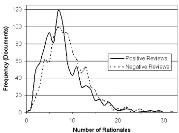
Figure 1: Histograms of rationale counts per document (A0’s annotations). The overall mean of 8.55 is close to that of the four annotators in Table 1. The median and mode are 8 and 7.
• A woman in peril. A confrontation. An explosion. The
end.Yawn. Yawn. Yawn.
• when a film makes watching Eddie Murphya tedious ex-perience, you know something is terribly wrong. • the movie isso badly put togetherthat even the most
casual viewer may notice themiserable pacing and stray plot threads.
• don’t go seethis movie
The annotation involvesboldfacingthe rationale phrases using an HTML editor. Note that a fancier annotation tool would be necessary for a task like named entity tagging, where an annotator must mark many named entities in a single document. At any given moment, such a tool should allow the annota-tor to highlight, view, and edit only the several ra-tionales for the “current” annotated entity (the one most recently annotated or re-selected).
One of the authors (A0) annotated folds 0–8 of the movie review set (1,800 documents) with ra-tionales that supported the gold-standard classifica-tions. This training/development set was used for all of the learning experiments in sections 5–6. A histogram of rationale counts is shown in Figure 1. As mentioned in section 3, the rationale annotations were just textual substrings. The annotator did not require knowledge of the classifier features. Thus, our rationale dataset is a new resource4 that could also be used to study exploitation of rationales un-der feature sets or learning methods other than those considered here (see section 8).
4.2 Inter-annotator agreement
doc-Rationales % rationales also % rationales also % rationales also % rationales also % rationales also per document annotated by A1 annotated by A2 annotated by AX annotated byAY ann. byanyone else
A1 5.02 (100) 69.6 63.0 80.1 91.4
A2 10.14 42.3 (100) 50.2 67.8 80.9
AX 6.52 49.0 68.0 (100) 79.9 90.9
[image:4.612.73.542.57.121.2]AY 11.36 39.7 56.2 49.3 (100) 75.5
Table 1: Average number of rationales and inter-annotator agreement for Tasks 2 and 3. A rationale by Ai(“I thinkthis is a great
movie!”) is considered to have been annotated also by Ajif at least one of Aj’s rationales overlaps it (“I think this is agreat movie!”). In computing pairwise agreement on rationales, we ignored documents where Aiand Ajdisagreed on the class. Notice that the most thorough annotatorAYcaught most rationales marked by the others (exhibiting high “recall”), and that most rationales enjoyed some degree of consensus, especially those marked by the least thorough annotatorA1(exhibiting high “precision”).
uments were split into three groups, each consisting of 50 documents (25 positive and 25 negative). Each subset was used for one of three tasks:6
• Task 1:Given the document, annotate only the class (positive/negative).
• Task 2: Given the document and its class, an-notate some rationales for that class.
• Task 3:Given the document, annotate both the class and some rationales for it.
We carried out a pilot study (annotators AX and AY: two of the authors) and a later, more controlled study (annotators A1 and A2: paid students). The latter was conducted in a more controlled environ-ment where both annotators used the same annota-tion tool and annotaannota-tion setup as each other. Their guidelines were also more detailed (see section 4.1). In addition, the documents for the different tasks were interleaved to avoid any practice effect.
The annotators’ classification accuracies in Tasks 1 and 3 (against Pang & Lee’s labels) ranged from 92%–97%, with 4-way agreement on the class for 89% of the documents, and pairwise agreement also ranging from 92%–97%. Table 1 shows how many rationales the annotators provided and how well their rationales agreed.
Interestingly, in Task 3, four of AX’s ratio-nales for a positive class were also partially highlighted by AY as support for AY’s (incorrect) negativeclassifications, such as:
6
Each task also had a “warmup” set of 10 documents to be annotated before that tasks’s 50 documents. Documents for Tasks 2 and 3 would automatically open in an HTML editor while Task 1 documents opened in an HTML viewer with no editing option. The annotators recorded their classifications for Tasks 1 and 3 on a spreadsheet.
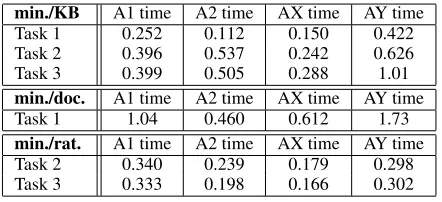
min./KB A1 time A2 time AX time AY time
Task 1 0.252 0.112 0.150 0.422
Task 2 0.396 0.537 0.242 0.626
Task 3 0.399 0.505 0.288 1.01
min./doc. A1 time A2 time AX time AY time
Task 1 1.04 0.460 0.612 1.73
min./rat. A1 time A2 time AX time AY time
Task 2 0.340 0.239 0.179 0.298
Task 3 0.333 0.198 0.166 0.302
Table 2: Average annotation rates on each task. • Even with its numerous flaws, the movie all comes
to-gether, if only for those who . . .
• “Beloved” acts like an incredibly difficult chamber drama paired with a ghost story.
4.3 Annotation time
Average annotation times are in Table 2. As hoped, rationales did not take too much extra time for most annotators to provide. For each annotator except A2, providing rationales only took roughly twice the time (Task 3 vs. Task 1), even though it meant mark-ing an average of 5–11 rationales in addition to the class.
Why this low overhead? Because marking the class already required the Task 1 annotator to read the document and find some rationales, even if s/he did not mark them. The only extra work in Task 3 is in making them explicit. This synergy between class annotation and rationale annotation is demon-strated by the fact that doing both at once (Task 3) was faster than doing them separately (Tasks 1+2).
We remark that this task—binary classification on full documents—seems to be almost a worst-case scenario for the annotation of rationales. At a purely mechanical level, it was rather heroic of A0 to at-tach 8–9 new rationale phrases rij to every bit yi
[image:4.612.317.538.202.303.2]lower-level annotationyiwill tend to have fewer
ra-tionalesrij, whileyiitself will be more complex and
hence more difficult to mark. Thus, we expect that the overhead of collecting rationales will be less in many scenarios than the factor of 2 we measured.
Annotation overhead could be further reduced. For a multi-class problem like relation detection, one could ask the annotator to provide rationalesonlyfor the rarer classes. This small amount of extra time where the data is sparsest would provide extra guid-ance where it was most needed. Another possibility is passive collection of rationales via eye tracking.
5 Experimental Procedures
5.1 Feature extraction
Although this dataset seems to demand discourse-level features that contextualize bits of praise and criticism, we exactly follow Pang et al. (2002) and Pang and Lee (2004) in merely using binary uni-gram features, corresponding to the 17,744 un-stemmed word or punctuation types with count≥4
in the full 2000-document corpus. Thus, each docu-ment is reduced to a 0-1 vector with 17,744 dimen-sions, which is then normalized to unit length.7
We used the method of section 3 to place addi-tional constraints on a linear classifier. Given a train-ing document, we create several contrast documents, each by deleting exactly one rationale substring from the training document. Converting documents to feature vectors, we obtained an original exam-ple −→xi and several contrast examples −v→i1,−v→i2, . . ..8
Again, our training method required each original document to be classified more confidently (by a marginµ) than its contrast documents.
If we were using more than unigram features, then simplydeleting a rationale substring would not al-ways be the best way to create a contrast document, as the resulting ungrammatical sentences might cause deep feature extraction to behave strangely (e.g., parse errors during preprocessing). The goal in creating the contrast document is merely to suppress
7
The vectors are normalizedbeforeprepending the 1 corre-sponding to the bias term feature (mentioned in section 3).
8
The contrast examples were not normalized to precisely unit length, but instead were normalized by the same factor used to normalize−→xi. This conveniently ensured that the pseudoex-amples−x→ij
def
= ~xi−−v→ij
µ were sparse vectors, with 0 coordinates for all words not in thejthrationale.
features (n-grams, parts of speech, syntactic depen-dencies . . . ) that depend in part on material in one or more rationales. This could be done directly by modifying the feature extractors, or if one prefers to use existing feature extractors, by “masking” rather than deleting the rationale substring—e.g., replacing each of its word tokens with a specialMASK token that is treated as an out-of-vocabulary word.
5.2 Training and testing procedures
We transformed this problem to an SVM problem (see section 3) and applied SVMlightfor training and testing, using the default linear kernel. We used only A0’s rationales and the true classifications.
Fold 9 was reserved as a test set. All accuracy results reported in the paper are the result of testing on fold 9, after training on subsets of folds 0–8.
Our learning curves show accuracy after training onT < 9folds (i.e.,200T documents), for various
T. To reduce the noise in these results, the accuracy we report for training onT folds is actually the aver-age of 9 different experiments with different (albeit overlapping) training sets that cover folds 0–8:
1 9
8
X
i=0
acc(F9 |θ∗, Fi+1∪. . .∪Fi+T) (7)
whereFj denotes the fold numberedj mod 9, and
acc(Z |θ, Y)means classification accuracy on the setZ after training onY with hyperparametersθ.
To evaluate whether two different training meth-ods A and B gave significantly different average-accuracy values, we used a paired permutation test (generalizing a sign test). The test assumes in-dependence among the 200 test examples but not among the 9 overlapping training sets. For each of the 200 test examples in fold 9, we measured
(ai, bi), where ai (respectively bi) is the number
of the 9 training sets under which A (respectively B) classified the example correctly. The p value is the probability that the absolute difference be-tween the average-accuracy values would reach or exceed the observed absolute difference, namely
| 1 200
P200
i=1
ai−bi
9 |, if each(ai, bi)had an independent
1/2 chance of being replaced with(bi, ai), as per the
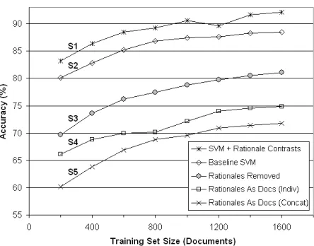
Figure 2: Classification accuracy under five different experi-mental setups (S1–S5). At each training size, the 5 accura-cies are pairwise significantly different (paired permutation test,
p < 0.02; see section 5.2), except for{S3,S4}or{S4,S5}at some sizes.
(C, µ, Ccontrast) to maximize the following cross-validation performance:9
θ∗= argmax θ
8
X
i=0
acc(Fi |θ, Fi+1∪. . .∪Fi+T)
(8) We used a simple alternating optimization procedure that begins atθ0 = (1.0,1.0,1.0)and cycles
repeat-edly through the three dimensions, optimizing along each dimension by a local grid search with resolu-tion 0.1.10 Of course, when training without ratio-nales, we did not have to optimizeµorCcontrast.
6 Experimental Results
6.1 The value of rationales
The top curve (S1) in Figure 2 shows that perfor-mance does increase when we introduce rationales for the training examples as contrast examples (sec-tion 3). S1 is significantly higher than the baseline curve (S2) immediately below it, which trains an or-dinary SVM classifier without using rationales. At the largest training set size, rationales raise the accu-racy from 88.5% to 92.2%, a 32% error reduction.
9
One might obtain better performance (acrossallmethods being compared) by choosing a separateθ∗for each of the 9 training sets. However, to simulate real limited-data training conditions, one should then find theθ∗for each{i, ..., j} us-ing a separate cross-validation within{i, ..., j}only; this would slow down the experiments considerably.
10
For optimizing along theCdimension, one could use the efficient method of Beineke et al. (2004), but not in SVMlight.
The lower three curves (S3–S5) show that learn-ing is separately helped by the rationale and the non-rationale portions of the documents. S3–S5 are degraded versions of the baseline S2: they are ordinary SVM classifiers that perform significantly worse than S2 (p <0.001).
Removing the rationale phrases from the train-ing documents (S3) made the test documents much harder to discriminate (compared to S2). This sug-gests that annotator A0’s rationales often covered mostof the usable evidence for the true class.
However, the pieces to solving the classification puzzle cannot be found solely in the short rationale phrases. Removing allnon-rationale text from the training documents (S5) was even worse than re-moving the rationales (S3). In other words, we can-not hope to do well simply by training on just the rationales (S5), although that approach is improved somewhat in S4 by treating each rationale (similarly to S1) as aseparateSVM training example.
This presents some insight into why our method gives the best performance. The classifier in S1 is able to extract subtle patterns from the corpus, like S2, S3, or any other standard machine learn-ing method, but it isalsoable to learn from a human annotator’s decision-making strategy.
6.2 Using fewer rationales
In practice, one might annotate rationales for only sometraining documents—either when annotating a new corpus or when adding rationales post hoc to an existing corpus. Thus, a range of options can be found between curves S2 and S1 of Figure 2.
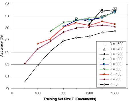
Figure 3 explores this space, showing how far the learning curve S2 moves upward if one has time to annotate rationales for a fixed number of documents
R. The key useful discovery is that much of the ben-efit can actually be obtained with relatively few ra-tionales. For example, with 800 training documents, annotating (0%, 50%, 100%) of them with rationales gives accuracies of (86.9%, 89.2%, 89.3%). With the maximum of 1600 training documents, annotat-ing (0%, 50%, 100%) with rationales gives (88.5%, 91.7%, 92.2%).
To make this point more broadly, we find that the
R = 200 curve is significantly above the R = 0
curve (p < 0.05) at allT ≤ 1200. By contrast, the
Figure 3: Classification accuracy forT ∈ {200,400, ...,1600} training documents (x-axis) when onlyR ∈ {0,200, ..., T}of them are annotated with rationales (different curves). TheR= 0curve above corresponds to the baseline S2 from Figure 2. S1’s points are found above as the leftmost points on the other curves, whereR=T.
value are all-pairs statistically indistinguishable. The figure also suggests that rationales and docu-ments may be somewhat orthogonal in their benefit. When one has many documents and few rationales, there is no longer much benefit in adding more doc-uments (the curve is flattening out), but adding more rationales seems to provide a fresh benefit: ratio-nales have not yet reachedtheirpoint of diminishing returns. (While this fresh benefit was often statisti-cally significant, and greater than the benefit from more documents, our experiments did not establish that it was significantly greater.)
The above experiments keepallof A0’s rationales ona fraction oftraining documents. We also exper-imented with keepinga fraction of A0’s rationales (chosen randomly with randomized rounding) onall training documents. This yielded no noteworthy or statistically significant differences from Figure 3.
These latter experiments simulate a “lazy annota-tor” who is less assiduous than A0. Such annotators may be common in the real world. We also suspect that they will be more desirable. First, they should be able to add more rationales per hour than the A0-style annotator from Figure 3: some rationales are simply more noticeable than others, and a lazy anno-tator will quickly find the most noticeable ones with-out wasting time tracking down the rest. Second, the “most noticeable” rationales that they mark may be the most effective ones for learning, although our
random simulation of laziness could not test that.
7 Related Work
Our rationales resemble “side information” in ma-chine learning—supplementary information about the target function that is available at training time. Side information is sometimes encoded as “virtual examples” like our contrast examples or pseudoex-amples. However, past work generates these by automatically transforming the training examples in ways that are expected to preserve or alter the classification (Abu-Mostafa, 1995). In another for-mulation, virtual examples are automatically gener-ated but must be manually annotgener-ated (Kuusela and Ocone, 2004). Our approach differs because a hu-man helps to generate the virtual examples. Enforc-ing a margin between ordinary examples and con-trast examples also appears new.
Other researchers have considered how to reduce annotation effort. In active learning, the annotator classifies only documents where the system so far is less confident (Lewis and Gale, 1994), or in an in-formation extraction setting, incrementally corrects details of the system’s less confident entity segmen-tations and labelings (Culotta and McCallum, 2005). Raghavan et al. (2005) asked annotators to iden-tify globally “relevant”features. In contrast, our ap-proach does not force the annotator to evaluate the importance of features individually, nor in a global context outside any specific document, nor even to know the learner’s feature space. Annotators only mark text that supports their classification decision. Our methods then consider the combined effect of this text on the feature vector, which may include complex features not known to the annotator.
8 Future Work: Generative models
Our SVM contrast method (section 3) is not the only possible way to use rationales. We would like to ex-plicitly model rationale annotation as a noisy pro-cess that reflects, imperfectly and incompletely, the annotator’s internal decision procedure.
A natural approach would start with log-linear models in place of SVMs. We can define a proba-bilistic classifier
pθ(y|x) def = 1
Z(x)exp k X
h=1
wheref~(·)extracts a feature vector from a classified document.
A standard training method would be to chooseθ
to maximize the conditional likelihood of the train-ing classifications:
argmax ~ θ
n Y
i=1
pθ(yi |xi) (10)
When a rationale ri is also available for each (xi, yi), we propose to maximize a likelihood that
tries to predict these rationale dataas well:
argmax ~ θ
n Y
i=1
pθ(yi |xi)·pθ0(ri|xi, yi, θ) (11)
Notice that a given guess ofθmight make equa-tion (10) large, yet accord badly with the annotator’s rationales. In that case, the second term of equa-tion (11) will exert pressure onθto change to some-thing that conforms more closely to the rationales. If the annotator is correct, such a θwill generalize better beyond the training data.
In equation (11),pθ0models the stochastic process of rationale annotation. What is an annotator actu-ally doing when she annotates rationales? In par-ticular, how do her rationales derive from the true value of θand thereby tell us aboutθ? Building a good modelpθ0 of rationale annotation will require some exploratory data analysis. Roughly, we expect that if θhfh(xi, y) is much higher for y = yi than
for other values ofy, then the annotator’sriis
corre-spondingly more likely to indicate in some way that feature fh strongly influenced annotationyi.
How-ever, we must also model the annotator’s limited pa-tience (she may not annotate all important features), sloppiness (she may indicate only indirectly thatfh
is important), and bias (tendency to annotate some kindsof features at the expense of others).
One advantage of this generative approach is that it eliminates the need for contrast examples. Con-sider a non-textual example in which an annotator highlights the line crossing in a digital image of the digit “8” to mark the rationale that distinguishes it from “0.” In this case it is not clear how to mask out that highlighted rationale to create a contrast exam-ple in which relevant features would not fire.11
11
One cannot simply flip those highlighted pixels to white
9 Conclusions
We have proposed a quite simple approach to im-proving machine learning by exploiting the clever-ness of annotators, asking them to provide enriched annotations for training. We developed and tested a particular discriminative method that can use “an-notator rationales”—even on a fraction of the train-ing set—to significantly improve sentiment classifi-cation of movie reviews.
We found fairly good annotator agreement on the rationales themselves. Most annotators provided several rationales per classification without taking too much extra time, even in our text classification scenario, where the rationales greatly outweigh the classifications in number and complexity. Greater speed might be possible through an improved user interface or passive feedback (e.g., eye tracking).
In principle, many machine learning methods might be modified to exploit rationale data. While our experiments in this paper used a discriminative SVM, we plan to explore generative approaches.
References
Y. S. Abu-Mostafa. 1995. Hints.Neural Computation, 7:639– 671, July.
P. Beineke, T. Hastie, and S. Vaithyanathan. 2004. The sen-timental factor: Improving review classification via human-provided information. InProc. of ACL, pages 263–270. A. L. Blum and R. L. Rivest. 1992. Training a 3-node neural
network is NP-complete.Neural Networks, 5(1):117–127. A. Culotta and A. McCallum. 2005. Reducing labeling effort
for structured prediction tasks. InAAAI, pages 746–751. S. Dumais. 1998. Using SVMs for text categorization. IEEE
Intelligent Systems Magazine, 13(4), July/August.
T. Joachims. 1998. Text categorization with support vector machines: Learning with many relevant features. InProc. of the European Conf. on Machine Learning, pages 137–142. P. Kuusela and D. Ocone. 2004. Learning with side
informa-tion: PAC learning bounds. J. of Computer and System Sci-ences, 68(3):521–545, May.
D. D. Lewis and W. A. Gale. 1994. A sequential algorithm for training text classifiers. InProc. of ACM-SIGIR, pages 3–12. B. Pang and L. Lee. 2004. A sentimental education: Sen-timent analysis using subjectivity summarization based on minimum cuts. InProc. of ACL, pages 271–278.
B. Pang, L. Lee, and S. Vaithyanathan. 2002. Thumbs up? Sentiment classification using machine learning techniques. InProc. of EMNLP, pages 79–86.
H. Raghavan, O. Madani, and R. Jones. 2005. Interactive fea-ture selection. InProc. of IJCAI, pages 41–46.