Tied Mixture Language Modeling in Continuous Space

Tied–Mixture Language Modeling in Continuous Space

Ruhi Sarikaya

IBM T.J. Watson Research Center Yorktown Heights, NY 10598 [email protected]

Mohamed Afify Orange Labs.

Cairo, Egypt

mohamed [email protected]

Brian Kingsbury

IBM T.J. Watson Research Center Yorktown Heights, NY 10598

[email protected]

Abstract

This paper presents a new perspective to the language modeling problem by moving the word representations and modeling into the continuous space. In a previous work we in-troduced Gaussian-Mixture Language Model (GMLM) and presented some initial experi-ments. Here, we propose Tied-Mixture Lan-guage Model (TMLM), which does not have the model parameter estimation problems that GMLM has. TMLM provides a great deal of parameter tying across words, hence achieves robust parameter estimation. As such, TMLM can estimate the probability of any word that has as few as two occurrences in the train-ing data. The speech recognition experiments with the TMLM show improvement over the word trigram model.

1 Introduction

Despite numerous studies demonstrating the serious short-comings of the n–gram language models, it has been surprisingly difficult to outperform n–gram language models consistently across different do-mains, tasks and languages. It is well-known that n– gram language models are not effective in modeling long range lexical, syntactic and semantic dependen-cies. Nevertheless, n–gram models have been very appealing due to their simplicity; they require only a plain corpus of data to train the model. The im-provements obtained by some more elaborate lan-guage models (Chelba & Jelinek, 2000; Erdogan et al., 2005) come from the explicit use of syntactic and semantic knowledge put into the annotated corpus.

In addition to the mentioned problems above, tra-ditional n–gram language models do not lend them-selves easily to rapid and effective adaptation and

discriminative training. A typical n–gram model contains millions of parameters and has no structure capturing dependencies and relationships between the words beyond a limited local context. These pa-rameters are estimated from the empirical distribu-tions, and suffer from data sparseness. n–gram lan-guage model adaptation (to new domain, speaker, genre and language) is difficult, simply because of the large number of parameters, for which large amount of adaptation data is required. Instead of up-dating model parameters with an adaptation method, the typical practice is to collect some data in the tar-get domain and build a domain specific language model. The domain specific language model is in-terpolated with a generic language model trained on a larger domain independent data to achieve ro-bustness. On the other hand, rapid adaptation for acoustic modeling, using such methods as Maxi-mum Likelihood Linear Regression (MLLR) (Leg-etter & Woodland, 1995), is possible using very small amount of acoustic data, thanks to the inher-ent structure of acoustic models that allow large de-grees of parameter tying across different words (sev-eral thousand context dependent states are shared by all the words in the dictionary). Likewise, even though discriminatively trained acoustic mod-els have been widely used, discriminatively trained languages models (Roark et al., 2007) have not widely accepted as a standard practice yet.

In this study, we present a new perspective to the language modeling. In this perspective, words are not treated as discrete entities but rather vectors of real numbers. As a result, long–term semantic re-lationships between the words could be quantified and can be integrated into a model. The proposed formulation casts the language modeling problem as

an acoustic modeling problem in speech recognition. This approach opens up new possibilities from rapid and effective adaptation of language models to using discriminative acoustic modeling tools and meth-ods, such as Minimum Phone Error (MPE) (Povey & Woodland, 2002) training to train discriminative language models.

We introduced the idea of language modeling in continuous space from the acoustic modeling per-spective and proposed Gaussian Mixture Language Model (GMLM) (Afify et al., 2007). However, GMLM has model parameter estimation problems. In GMLM each word is represented by a specific set of Gaussian mixtures. Robust parameter estimation of the Gaussian mixtures requires hundreds or even thousands of examples. As a result, we were able to estimate the GMLM probabilities only for words that have at least 50 or more examples. Essentially, this was meant to estimate the GMLM probabilities for only about top 10% of the words in the vocab-ulary. Not surprisingly, we have not observed im-provements in speech recognition accuracy (Afify et al., 2007). Tied-Mixture Language Model (TMLM) does not have these requirements in model estima-tion. In fact, language model probabilities can be es-timated for words having as few as two occurrences in the training data.

The concept of language modeling in continuous space was previously proposed (Bengio et al., 2003; Schwenk & Gauvain, 2003) using Neural Networks. However, our method offers several potential advan-tages over (Schwenk & Gauvain, 2003) including adaptation, and modeling of semantic dependencies because of the way we represent the words in the continuous space. Moreover, our method also al-lows efficient model training using large amounts of training data, thanks to the acoustic modeling tools and methods which are optimized to handle large amounts of data efficiently.

It is important to note that we have to realize the full potential of the proposed model, before investi-gating the potential benefits such as adaptation and discriminative training. To this end, we propose TMLM, which does not have the problems GMLM has and, unlike GMLM we report improvements in speech recognition over the corresponding n–gram models.

The rest of the paper is organized as follows.

Sec-tion 2 presents the concept of language modeling in continuous space. Section 3 describes the tied– mixture modeling. Speech recognition architecture is summarized in Section 4, followed by the experi-mental results in Section 5. Section 6 discusses var-ious issues with the proposed method and finally, Section 7 summarizes our findings.

2 Language Modeling In Continuous Space

The language model training in continuous space has three main steps; namely, creation of a co– occurrence matrix, mapping discrete words into a continuous parameter space in the form of vectors of real numbers and training a statistical parametric model. Now, we will describe each step in detail.

2.1 Creation of a co–occurrence Matrix

There are many ways that discrete words can be mapped into a continuous space. The ap-proach we take is based on Latent Semantic Analy-sis (LSA) (Deerwester et al., 1990), and begins with the creation of a co–occurrence matrix. The co–occurrence matrix can be constructed in sev-eral ways, depending on the morphological com-plexity of the language. For a morphologically impoverished language, such as English the co– occurrence matrix can be constructed using word bi-gram co–occurrences. For morphologically rich lan-guages, there are several options to construct a co– occurrence matrix. For example, the co–occurrence matrix can be constructed using either words (word– word co–occurrences) or morphemes (morpheme– morpheme co–occurrences), which are obtained af-ter morphologically tokenizing the entire corpus. In addition to word–word or morpheme–morpheme co–occurrence matrices, a word–morpheme co– occurrence matrix can also be constructed. A word

w can be decomposed into a set of prefixes, stem

and suffixes:w= [pf x1+pf x2+pf xn+stem+

In this study, we use morpheme level bigram co– occurrences to construct the matrix. All the mor-pheme1 _{bigrams are accumulated for the entire}

cor-pus to fill in the entries of a co–occurrence matrix,

C, whereC(wi, wj) denotes the counts for which word wi follows wordwj in the corpus. This is a large, but very sparse matrix, since typically a small number of words follow a given word. Because of its large size and sparsity, Singular Value Decom-position (SVD) is a natural choice for producing a reduced-rank approximation of this matrix.

The co–occurrence matrices typically contain a small number of high frequency events and a large number of less frequent events. Since SVD derives a compact approximation of the co–occurrence ma-trix that is optimal in the least–square sense, it best models these high-frequency events, which may not be the most informative. Therefore, the entries of a word-pair co–occurrence matrix are smoothed ac-cording to the following expression:

ˆ

C(wi, wj) = log(C(wi, wj) + 1) (1)

Following the notation presented in (Bellegarda, 2000) we proceed to perform the SVD as follows:

ˆ

C≈U SVT (2)

whereU is a left singular matrix with row vectors

ui (1 ≤ i ≤ M) and dimensionM ×R. S is a diagonal matrix of singular values with dimension

R_×R.V is a right singular matrix with row vectors

vj (1 ≤ j ≤ N) and dimension N ×R. R is the order of the decomposition andR _¿ min(M, N). M and N are the vocabulary sizes on the rows and columns of the co–occurrence matrix, respec-tively. For word–word or morpheme–morpheme co–occurrence matrices M = N, but for word– morpheme co–occurrence matrix,M is the number

of unique words in the training corpus andN is the

number of unique morphemes in morphologically tokenized training corpus.

2.2 Mapping Words into Continuous Space The continuous space for the words listed on the rows of the co–occurrence matrix is defined as the space spanned by the column vectors ofAM×R =

1_{For the generality of the notation, from now on we use}

“word” instead of “morpheme”.

U S. Similarly, the continuous space for the words

on the columns are defined as the space spanned by the row vectors ofB_R×N = SVT. Here, for

a word–word co–occurrence matrix, each of the scaled vectors (byS) in the columns ofAand rows ofB are called latent word history vectors for the

forward and backward bigrams, respectively. Now, a bigramwij = (wi, wj)(1 ≤ i, j ≤ M) is repre-sented as a vector of dimensionM ×1, where the

ithentry ofwij is 1 and the remaining ones are zero. This vector is mapped to a lower dimensional vector

ˆ

wij by:

ˆ

wij =ATwij (3)

wherewˆij has dimension ofR ×1. Similarly, the backward bigramwji(1≤j, i≤N) is mapped to a lower dimensional vectorwˆjiby:

ˆ

wji =Bwji (4)

wherewˆji has dimension ofR×1. Note that for a word–morpheme co–occurrence matrix the rows of

Bwould contain latent morpheme vectors.

Since a trigram history consists of two bigram his-tories, a trigram history vector is obtained by con-catenating two bigram vectors. Having generated the features, now we explain the structure of the parametric model and how to train it for language modeling in continuous space.

2.3 Parametric Model Training in Continuous Space

Recalling the necessary inputs to train an acoustic model for speech recognition would be helpful to explain the new language modeling method. The acoustic model training in speech recognition needs three inputs: 1) features (extracted from the speech waveform), 2) transcriptions of the speech wave-forms and 3) basewave-forms, which show the pronuncia-tion of each word in the vocabulary. We propose to model the language model using HMMs. The HMM parameters are estimated in such way that the given set of observations is represented by the model in the “best” way. The “best” can be defined in vari-ous ways. One obvivari-ous choice is to use Maximum Likelihood (ML) criterion. In ML, we maximize the probability of a given sequence of observationsO,

This probability is the total likelihood of the obser-vations and can be expressed mathematically as:

Ltot =p(O|λ) (5)

However, there is no known way to analytically solve for the modelλ = _{A, B, π_} , which max-imize the quantity Ltot, where A is the transi-tion probabilities, B is the observation

probabili-ties, and π is the initial state distribution. But we can choose model parameters such that it is locally maximized, using an iterative procedure, like Baum-Welch method (Baum et al., 1970).

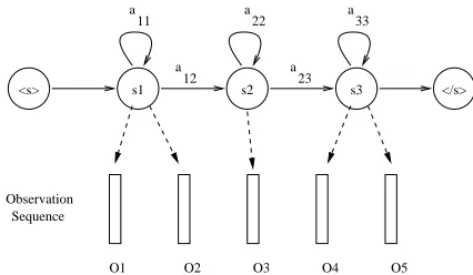
The objective function given in Eq. 5 is the same objective function used to estimate the parameters of an HMM based acoustic model. By drawing an analogy between the acoustic model training and language modeling in continuous space, the history vectors are considered as the acoustic observations (feature vectors) and the next word to be predicted is considered as the label the acoustic features belong to, and words with their morphological decomposi-tions can be considered as the lexicon or dictionary. Fig. 1 presents the topology of the model for model-ing a word sequence of 3 words. Each word is mod-eled with a single state left–to–right HMM topology. Using a morphologically rich language (or a char-acter based language like Chinese) to explain how HMMs can be used for language modeling will be helpful. In the figure, let the states be the words and the observations that they emit are the morphemes (or characters in the case of Chinese). The same topology (3 states) can also be used to model a sin-gle word, where the first state models the prefixes, the middle state models the stem and the final state models the suffixes. In this case, words are repre-sented by network of morphemes. Each path in a word network represents a segmentation (or “pro-nunciation”) of the word.

The basic idea of the proposed modeling is to cre-ate a separcre-ate model for each word of the language and use the language model corpus to estimate the parameters of the model. However, one could argue that the basic model could be improved by taking the contexts of the morphemes into account. Instead of building a single HMM for each word, several models could be trained according to the context of the morphemes. These models are called context–

<s> s1 s2 s3 </s> a

11

a 12

22 a

a 23

a 33

Observation Sequence

O1 O2 O3 O4 O5

Figure 1: HMM topology for language modeling in con-tinuous space.

dependent morphemes. The most obvious choice is to use both left and right neighbor of a morpheme as context, and creating, what we call tri–morphemes. In principal even if context-dependent morphemes could improve the modeling accuracy, the number of models increase substantially. For a vocabulary size ofV, the number of tri–morpheme could be as high asV3. However, most of the tri–morphemes

are either rare or will not be observed in the training data altogether.

Decision tree is one approach that can solve this problem. The main idea is to find similar tri– morphemes and share the parameters between them. The decision tree uses a top-down approach to split the samples, which are in a single cluster at the root of the tree, into smaller clusters by asking questions about the current morpheme and its context. In our case, the questions could be syntactic and/or seman-tic in nature.

What we hope for is that in the new continuous space there is some form of distance or similarity between histories such that histories not observed in the data for some words are smoothed by similar ob-served histories.

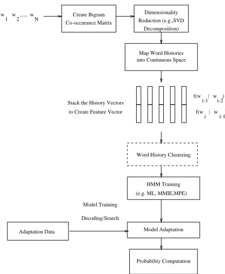
ma-trix is decomposed using SVD. The columns of the left–singular matrix obtained from SVD is used to map the bigram word histories into a lower dimen-sional continuous parameter space. The projected word history vectors are stacked together depending on the size of the n–gram. For example, for trigram modeling two history vectors are stacked together. Even though, we have not done so, at this stage one could cluster the word histories for robust parame-ter estimation. Now, the feature vectors, their corre-sponding transcriptions and the lexicon (baseforms) are ready to perform the “acoustic model training”. One could use maximum likelihood criterion or any other objective function such as Minimum Phone Er-ror (MPE) training to estimate the language model parameters in the continuous space.

The decoding phase could employ an adaptation step, if one wants to adapt the language model to a different domain, speaker or genre. Then, given a hypothesized sequence of words the decoder ex-tracts the corresponding feature vectors. The fea-ture vectors are used to estimate the likelihood of the word sequence using the HMM parameters. This likelihood is used to compute the probability of the word sequence. Next, we introduce Tied–Mixture Modeling, which is a special HMM structure to ro-bustly estimate model parameters.

3 Tied–Mixture Modeling

Hidden Markov Models (HMMs) have been exten-sively used virtually in all aspects of speech and language processing. In speech recognition area continuous-density HMMs have been the standard for modeling speech signals, where several thousand context–dependent states have their own Gaussian density functions to model different speech sounds. Typically, speech data have hundreds of millions of frames, which are sufficient to robustly estimate the model parameters. The amount of data for language modeling is orders of magnitude less than that of the acoustic data in continuous space. Tied–Mixture Hidden Markov Models (TM–HMMs) (Bellegarda & Nahamoo, 1989; Huang & Jack, 1988) have a bet-ter decoupling between the number of Gaussians and the number of states compared to continuous den-sity HMMs. The TM–HMM is useful for language modeling because it allows us to choose the

num-HMM Training (e.g. ML, MMIE,MPE)

Model Adaptation Decoding/Search

Model Training

Word History Clustering

Adaptation Data

Probability Computation N

w 1

to Create Feature Vector ,...,

2 w

w Dimensionality Reduction (e.g.,SVD

Decomposition) Create Bigram

Co-occurance Matrix

Map Word Histories into Continuous Space

i-2 i-1

i-1 i f(w | w )

f(w | w ) Stack the History Vectors

Figure 2: Language Model Training and Adaptation in Continuous Space.

ber of Gaussian densities and the number of mixture weights independently. Much more data is required to reliably estimate Gaussian densities than to esti-mate mixture weights.

The evaluation of the observation density func-tions for TM–HMMs can be time consuming due to the large mixture weight vector and due to the fact that for each frame all Gaussians have to be evalu-ated. However, there are a number of solutions pro-posed in the past that significantly reduces the com-putation (Duchateau et al., 1998).

The function p(w | h), defined in a

continu-ous space, represents the conditional probability of the word w given the history h. In general, h

state in which a single set of Gaussians is shared among all states:

p(o|w) =

J

X

j

cw,jNj(o, µw,j,Σw,j) (6)

wherewis the state,_Nj is thejth Gaussian, ando is the observation (i.e. history) vectors. andJ is the

number of component mixtures in the TM-HMM. In order to avoid zero variance in word mapping into continuous space, all the latent word vectors are added a small amount of white noise.

The TM–HMM topology is given in Fig. 3. Each state models a word and they all share the same set of Gaussian densities. However, each state has a spe-cific set of mixture weights associated with them. This topology can model a word–sequence that con-sist of three words in them. The TM–HMM esti-mates the probability of observing the history vec-tors (h) for a given wordw. However, what we need

is the posterior probabilityp(w _|h)of observingw

as the next word given the history,h. This can be obtained using the Bayes rule:

p(w|h) = p(h|w)p(w)

p(h) (7)

= _PVp(h|w)p(w)

v=1p(h|v)p(v)

(8)

wherep(w) is the unigram probability of the word w. The unigram probabilities can also be substituted

for more accurate higher order n–gram probabilities. If this n–gram has an order that is equal to or greater than the one used in defining the continuous contexts

h, then the TMLM can be viewed as performing a

kind of smoothing of the original n–gram model:

Ps(w|h) =

P(w_|h)p(h_|w) PV

v=1P(v|h)p(h|v)

(9)

where Ps(w | h) andP(w | h) are the smoothed and original n–grams.

The TM–HMM parameters are estimated through an iterative procedure called the Baum-Welch, or forward-backward, algorithm (Baum et al., 1970). The algorithm locally maximizes the likelihood function via an iterative procedure. This type of

33

<s> s1 s2 s3 </s>

a 11

a 12

22 a

a 23

a

Figure 3: Tied-Mixture HMM topology for language modeling in continuous space. The mixtures are tied across states. Each state represents a word. The TM-HMM is completely defined with the mixture weights, mixture densities and transition probabilities.

training is identical to training continuous density HMMs except the Gaussians are tied across all arcs. For the model estimation equations the readers are referred to (Bellegarda & Nahamoo, 1989; Huang & Jack, 1988).

Next, we introduce the speech recognition system used for the experiments.

4 Speech Recognition Architecture

The speech recognition experiments are carried out on the Iraqi Arabic side of an English to Iraqi Ara-bic speech-to-speech translation task. This task cov-ers the military and medical domains. The acoustic data has about 200 hours of conversational speech collected in the context of a DARPA supported speech-to-speech (S2S) translation project (Gao et al., 2006).

2005). The baseline speech recognition system used in our experiments is the state–of–the–art and pro-duces a competitive performance.

The phone set consists of 33 graphemes represent-ing speech and silence for acoustic modelrepresent-ing. These graphemes correspond to letters in Arabic plus si-lence and short pause models. Short vowels are im-plicitly modeled in the neighboring graphemes. Fea-ture vectors are first aligned, using initial models, to model states. A decision tree is then built for each state using the aligned feature vectors by ask-ing questions about the phonetic context; quinphone questions are used in this case. The resulting tree has about 3K leaves. Each leaf is then modeled using a Gaussian mixture model. These models are first bootstrapped and then refined using three iterations of forward–backward training. The current system has about 75K Gaussians.

The language model training data has 2.8M words with 98K unique words and it includes acoustic model training data as a subset. The morpholog-ically analyzed training data has 58K unique vo-cabulary items. The pronunciation lexicon consists of the grapheme mappings of these unique words. The mapping to graphemes is one-to-one and there are very few pronunciation variants that are sup-plied manually mainly for numbers. A statistical tri-gram language model using Modified Kneser-Ney smoothing (Chen& Goodman, 1996) has been built using the training data, which is referred to as Word-3gr.

For decoding a static decoding graph is com-piled by composing the language model, the pro-nunciation lexicon, the decision tree, and the HMM graphs. This static decoding scheme, which com-piles the recognition network off–line before decod-ing, is widely adopted in speech recognition (Ri-ley et al., 2002). The resulting graph is further op-timized using determinization and minimization to achieve a relatively compact structure. Decoding is performed on this graph using a Viterbi beam search.

5 Experimental Results

We used the following TMLM parameters to build the model. The SVD projection size is set to 200 (i.e. R = 200) for each bigram history. This re-sults into a trigram history vector of size 400. This

−8 −7 −6 −5 −4 −3 −2 −1 0

−9 −8 −7 −6 −5 −4 −3 −2 −1 0

N−gram Probability

TMLM Probability

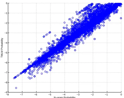
Figure 4: Scatter plot of the n–gram and TMLM proba-bilities.

vector is further projected down to a 50 dimensional feature space using LDA transform. The total num-ber of Gaussian densities used for the TM–HMM is set to 1024. In order to find the overall relationship between trigram and TMLM probabilities we show the scatter plot of the trigram and TMMT probabili-ties in Fig. 4. While calculating the TMLM score the TMLM likelihood generated by the model is divided by 40 to balance its dynamic range with that of the n–gram model. Most of the probabilities lie along the diagonal line. However, some trigram proba-bilities are modulated making TMLM probaproba-bilities quite different than the corresponding trigram prob-abilities. Analysis of TMLM probabilities with re-spect to the trigram probabilities would be an inter-esting future research.

LM TestA TestB TestC All

Word-3gr 18.7 18.6 38.9 32.9

TMLM 18.8 18.9 38.2 32.5

TMLM + Word-3gr 17.6 18.0 37.4 31.9

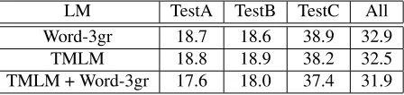
Table 1: Speech Recognition Language Model Rescoring Results.

In order to evaluate the performance of the TMLM, a lattice with a low oracle error rate was generated by a Viterbi decoder using the word tri-gram model (Word-3gr) model. From the lattice at most 30 (N=30) sentences are extracted for each ut-terance to form an N-best list. The N–best error rate for the combined test set (All) is 22.7%. The N– best size is limited (it is not in the hundreds), simply because of faster experiment turn-around. These ut-terances are rescored using TMLM. The results are presented in Table 1. The first two rows in the ta-ble show the baseline numbers for the word trigram (Word–3gr) model. TestA has a WER of 18.7% sim-ilar to that of TestB (18.6%). The WER for TestC is relatively high (38.9%), because, as explained above, TestC contains causal conversation with hes-itations and repairs, and speakers do not necessar-ily stick to the domain. Moreover, when users are speaking to a device, as in the case of TestA and TestB, they use clear and shorter sentences, which are easier to recognize. The TMLM does not pro-vide improvements for TestA and TestB but it im-proves the WER by 0.7% for TestC. The combined overall result is a 0.4% improvement over base-line. This improvement is not statistically signifi-cant. However, interpolating TMLM with Word-3gr improves the WER to 31.9%, which is 1.0% better than that of the Word-3gr. Standard p-test (Matched Pairs Sentence-Segment Word Error test available in standard SCLITEs statistical system comparison program from NIST) shows that this improvement is significant atp < 0.05 level. The interpolation

weights are set equally to 0.5 for each LM.

6 Discussions

Despite limited but encouraging experimental re-sults, we believe that the proposed perspective is a radical departure from the traditional n–gram based language modeling methods. The new perspective

opens up a number of avenues which are impossible to explore in one paper.

We realize that there are a number of outstand-ing issues with the proposed perspective that re-quire a closer look. We make a number of deci-sions to build a language model within this perspec-tive. The decisions are sometimes ad hoc. The de-cisions are made in order to build a working sys-tem and are by no means the best decisions. In fact, it is quite likely that a different set of de-cisions may result into a better system. Using a word–morpheme co–occurrence matrix instead of a morpheme–morpheme co–occurrence matrix is one such decision. Another one is the clustering/tying of the rarely observed events to achieve robust para-meter estimation both for the SVD and TMLM pa-rameter estimation. We also use a trivial decision tree to build the models where there were no con-text questions. Clustering morphemes with respect to their syntactic and semantic context is another area which should be explored. In fact, we are in the process of building these models. Once we have realized the full potential of the baseline maximum likelihood TMLM, then we will investigate the dis-criminative training methods such as MPE (Povey & Woodland, 2002) to further improve the language model performance and adaptation to new domains using MLLR (Legetter & Woodland, 1995).

We also realize that different problems such as segmentation (e.g. Chinese) of words or morpholog-ical decomposition of words into morphemes can be addressed within the proposed perspective.

7 Conclusions

References

M.Afify, O. Siohan and R. Sarikaya. 2007. Gaussian Mixture Language Models for Speech Recognition, ICASSP, Honolulu, Hawaii.

C.J. Legetter and P.C. Woodland. 1995. Maximum like-lihood linear regression for speaker adaptation of con-tinuous density hidden Markov models, Computer Speech and Language, vol.9, pp. 171-185.

J. Bellegarda. 2000. Large Vocabulary Speech Recogni-tion with Multispan Language Models, IEEE Trans-actions on Speech and Audio Processing, vol. 8, no. 1, pp. 76-84.

H. Schwenk, and J.L. Gauvain. 2003. Using Continuous Space Language Models for Conversational Telephony Speech Recognition, IEEE Workshop on Spontaneous Speech Processing and Recognition, Tokyo, Japan. J. Duchateau, K. Demuynck, D.V. Compernolle and P.

Wambacq. 1998. Improved Parameter Tying for Ef-ficient Acoustic Model Evaluation in Large Vocabu-lary Continuous Speech Recognition. Proc. of ICSLP, Sydney, Australia.

Y. Gao, L. Gu, B. Zhou, R. Sarikaya, H.-K. Kuo. A.-V.I. Rosti, M. Afify, W. Zhu. 2006. IBM MASTOR: Multilingual Automatic Speech-to-Speech Translator. Proc. of ICASSP, Toulouse, France.

S. Chen, J. Goodman. 1996. An Empirical Study of Smoothing Techniques for Language Modeling, ACL, Santa Cruz, CA.

J. Bellagarda and D. Nahamoo. 1989. Tied mixture con-tinuous parameter models for large vocabulary isolated speech recognition, Proc. of ICASSP, pp. 13-16. X.D. Huang and M.A. Jack. 1988. Hidden Markov

Mod-elling of Speech Based on a Semicontinuous Model, Electronic Letters, 24(1), pp. 6-7, 1988.

D. Povey and P.C. Woodland. 2002. Minimum phone er-ror and I-smoothing for improved discriminative train-ing,Proc. of ICASSP, pp. 105–108, Orlando, Florida. D. Povey, B. Kingsbury, L. Mangu, G. Saon, H. Soltau,

G. Zweig. 2005. fMPE: Discriminatively Trained Features for Speech Recognition, Proc. of ICASSP, pp. 961–964, Philadelphia, PA.

C. Chelba and F. Jelinek. 2000. Structured language modeling, Computer Speech and Language, 14(4), 283–332, 2000.

H. Erdogan, R. Sarikaya, S.F. Chen, Y. Gao and M. Picheny. 2005. Using Semantic Analysis to Improve Speech Recognition Performance, Computer Speech & Language Journal, vol. 19(3), pp: 321–343. B. Roark, M. Saraclar, M. Collins. 2007. Using

Seman-tic Analysis to Improve Speech Recognition Perfor-mance,Computer Speech & Language, vol. 21(2), pp: 373–392.

M. Riley, E. Bocchieri, A. Ljolje and M. Saraclar. 2007. The AT&T 1x real-time Switchboard speech-to-text system, NIST RT02 Workshop, Vienna, Virginia. Y. Bengio, R. Ducharme, P. Vincent and C. Jauvin. 2003.

A Neural Probabilistic Language Model. Journal of Machine Learning Research, vol. 3, 11371155. S. Deerwester, Susan Dumais, G. W. Furnas, T. K.

Lan-dauer, R. Harshman. 1990. Indexing by Latent Se-mantic Analysis, Journal of the American Society for Information Science, 41 (6): 391–407.