Conditions on abruptness in a gradient-ascent Maximum Entropy learner
∗Elliott Moreton
University of North Carolina, Chapel Hill [email protected]
Abstract
When does a gradual learning rule translate into gradual learningperformance? This pa-per studies a gradient-ascent Maximum En-tropy phonotactic learner, as applied to two-alternative forced-choice performance ex-pressed as log-odds. The main result is that slow initial performance cannot acceler-ate lacceler-ater if the initial weights are near zero, but can if they are not. Stated another way, abrupt-ness in this learner is an effect of transfer, ei-ther from Universal Grammar in the form of an initial weighting, or from previous learning in the form of an acquired weighting.
1 Introduction
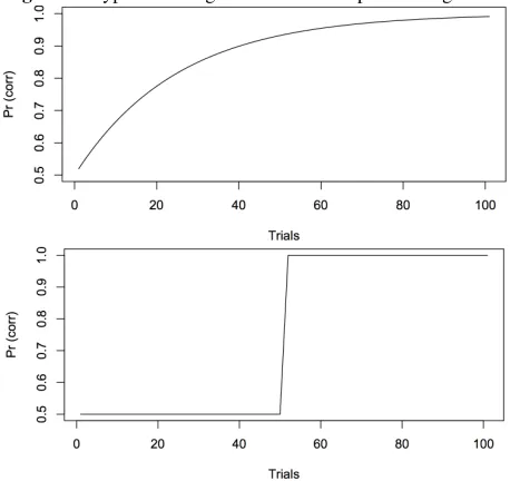
An important class of constraint-based phonologi-cal learning models responds to training by mak-ing small changes in the weight or rank of con-straints (reviewed in Jarosz 2016). The gradualness of the learning rule seems to suggest that perfor-mance ought to change gradually as well, resem-bling the first rather than the second panel in Figure 1. In work on non-linguistic pattern learning, abrupt improvement has been cited as diagnostic of an ex-plicit, “rule-based” learning algorithm which seri-ally tests hypotheses, as opposed to a “cue-based” one which slowly learns association weights (Ashby et al., 1998; Love, 2002; Maddox and Ashby, 2004; Smith et al., 2012; Kurtz et al., 2013). Abruptness
∗The author is indebted to Jen Smith, Joe Pater, Katya Pertsova, and Chris Wiesen for comments and suggestions. Any errors are of the author’s own making. The research was sup-ported in part by NSF BCS 1651105, “Inside phonological learning”, to E. Moreton and K. Pertsova.
has been found to correlate with other indicia of ex-plicitness by humans learning artificial phonology (Moreton and Pertsova, 2016).
[image:1.612.312.541.451.667.2]In fact, performance can change abruptly in grad-ual learners (Elman et al. 1996, Ch. 3–4; GLA ex-amples in Boersma 1998, Figure 14.25; Boersma and Levelt 2000; Jesney 2016). When does a gradual learning rule entail gradual learning performance? Could the model spend many trials invisibly inch-ing its way around to some point in weight space from which it can suddenly accelerate? Conversely, if we observe abrupt improvement in human learn-ers, does that disconfirm the model?
Figure 1:Hypothetical “gradual” and “abrupt” learning curve.
This paper addresses the question in a particu-larly basic case, that of a Maximum Entropy phono-tactic learner with a fixed constraint set that uses
113
gradient ascent on log-likelihood, no prior, and no restrictions on weights, and that makes two-alternative forced-choice (2AFC) decisions using the Luce choice rule. Gradient ascent Max-Ent is of interest not only in its own right, but because of its close relation to the Gradual Learning Algo-rithms for Stochastic Optimality Theory, Harmonic Grammar and Noisy Harmonic Grammar, and mod-els of non-linguistic learning such as the Perceptron (Boersma and Hayes, 2001; Fischer, 2005; J¨ager, 2007; Johnson, 2007; Pater, 2008; Pater and More-ton, 2012; Boersma and Pater, 2016; Moreton et al., 2017).
The results can be summarized as follows: Re-gardless of what the constraints actually are, if the initial weights are exactly zero then — provided that the training and test distributions are chosen in a par-ticular way — 2AFC performance improves fastest at the outset of learning, making abrupt learning im-possible. Even if, instead, the initial weights are onlynearzero, the 2AFC learning curve tracks that of a learner whose initial weights areexactly zero, in that the two learners’ trajectories in weight space steadily converge, and the closer they are in weight space, the more similar their 2AFC performance is. An example is given to show that largenon-zero ini-tial weights can, but need not, lead to abrupt 2AFC performance.
2 Learner and experimental scenario The universe of candidates is a finite set X = {x1, . . . , xn}, known to the experimenter. The model uses an unobservable set of constraints
c1, . . . , cm and an unobservable weight vectorw=
(w1, . . . , wm) to assign unobservable probabilities p = (p1, . . . , pn) to the candidate. This is done as follows (Goldwater and Johnson, 2003; J¨ager, 2007; Hayes and Wilson, 2008):
The harmony of a candidatexj is defined as the sum of its score vector, weighted by the current weights:
hw(xj) = m
X
i=1
wici(xj) (1)
The model’s estimate of the probabilitypj of can-didatexj is the exponential of its harmony, divided by the summed exponentials of the harmonies of all representations:
Zw= n
X
j=1
exphw(xj) (2)
Pr(X =xj |w) =
exphw(xj)
Zw (3)
The experimenter can at any time give the model a two-alternative forced-choicetest, in which two can-didatesxiandxj are presented to the model, which choosesxiwith probability
Pr(xi|(xi, xj)) =
pi
pi+pj (4)
This is the Luce choice rule (Luce, 1959, 23). The test is assumed not to change the state of the model. At the beginning of the experiment, the experi-menter chooses two probability distributionsr+and r−. On each test trial, one candidate is sampled from X with probabilities given by r+, and the other is
sampled fromXwith probabilities given byr−. The experimenter can also train the model by giving it a candidate xi as an example of a le-gal word. Instead of training on individual candi-dates (stochastic gradient ascent), we instead run the learner in batch mode (gradient ascent); i.e., instead of a candidate on each trial, the learner receives a distributionp+, wherep+i corresponds to the
proba-bility of presentingxion a stochastic gradient ascent training trial.
The model updates its weights according to the following rule:
∆wi =θ·(Ep+[ci]−Ew[ci]) (5)
This the Maximum Entropy gradient-ascent up-date rule, as described by J¨ager (2007). Its contribu-tion to the update is independent ofp−, the proba-bilities of the negative training candidates; i.e., the learner does “unsupervised” learning.
Below a continuous approximation to this discrete update rule is used, substituting dwi/dt for ∆wi. The learning rate parameterηis omitted by setting it
2001) or adaptively (Boyd and Vandenberghe, 1999, Section 5.2.1).
In this paper, “abrupt” is used to mean that perfor-mance improves slowly at the outset of the experi-ment, then accelerates later (e.g., a sigmoid). Perfor-mance is expressed here as log-odds rather than pro-portion correct because (A) log-odds is more trans-parently related both to the learning model (J¨ager, 2007) and to the statistical models fit to experimen-tal results (Jaeger, 2008), and (B) proportion correct acts as a squashing function, reducing the visible in-fluence of changing large weights and thus exagger-ating the effect whose existence we are arguing for on other grounds.
3 Improvement in log-likelihood decelerates monotonically
We begin by establishing a result that is almost what we want:
Proposition 1. Let L(t) = Pnj=1p+j logpj(t) de-note the model’s expectation of the log-likelihood of the empirical distribution at time t (Berger et al.,
1996). Then L(t) is always increasing but never accelerating; i.e., for anyt ≥ 0, dL/dt ≥ 0 and
d2L/dt2≤0.
Proof. We convert the learner to its Replicator form (Moreton et al., 2017):
d
dtlogpi= (C
TCe)
j−pTCTCe (6)
where C is the matrix1 whose (i, j)-th entry is ci(xj), ande = p+−p. Differentiating the defi-nition ofL(t)then yields
dL
dt =
n
X
j=1
p+j d
dtlogpj
=
n
X
j=1
p+j((CTCe)j−pTCTCe))
=(p+−p)TCTCe
=eTCTCe
=kCek2
(7)
1Note difference from familiar tableaus: RowsofC
corre-spond to constraints, andcolumnsto candidates.
(In this paper, k · k is the usual Euclidean norm.)
Since CTC is positive semidefinite, dL/dt ≥ 0. That confirms what we already know, since the learner does gradient ascent on L. The second
derivative is
d2L
dt2 =
d dte
TCTCe
=2eCTC
d dte
=−2
X
j
pj(CTCe)2j−
X
j
(pj(CTCe)j)2
=−2X
j
pj(1−pj)(CTCe)2j
(8)
Since0< pj <1, the sum is positive unlesse=0. Hence d2L/dt2 ≤0— the log-likelihood is always
increasing, but always more and more slowly, until it stops.
Regardless of the constraint set, initial state, tar-get pattern, or model parameters, learning, measured as log-likelihood, only ever slows down. Abrupt, sigmoidal, or U-shaped L(t) curves are not
possi-ble. However, what the experiments measure is not log-likelihood, which depends only on the probabil-ity assigned by the model to the winners, but rather 2AFC performance, which depends in part on how it distributes probability among the losing candidates. The next section addresses that complication.
4 When initial weights are all zero, initial improvement bounds later improvement In typical “artificial-language” experiments, the training and testing stimuli are, or approximate, ran-dom samples from the same distribution, and are presented to participants with equal frequency. We consider here a slightly more general possibility: Proposition 2. Suppose the experimenter chooses p+,r+, andr−such that at timet= 0, we have
p+−p(0) =α(r+−r−) (9)
for someα >0. Letλ+,−be the log-odds of a
d
dtEw[λ+,−]
t
≤ ddtEw[λ+,−] 0 (10)
Proof. For a given weight vector w, the expected harmony of a positive test candidate is
Ew,r+[hw(x+)] =
X
j
r+j hw(xj)
=X
j
r+j X
i
wici(xj)
! =X i wi X j
r+j ci(xj)
=X
i
wiEr+[ci]
(11)
i.e, the expected harmony of a positive test candidate is the weighted-by-the-weights sum of the average score on each constraint among positive test candi-dates. In terms ofC, the matrix whose(i, j)-th entry
isci(xj), we can write this as
Ew,r+[hw(x+)] =
X
i
wi(Cr+)i
=wTCr+
(12)
The same holds, mutatis mutandis, for negative test candidates. For any test pair (xi, xj), the log-odds λi,j of choosing xi is, by Equation 3, just the difference in harmony scores given the current weighting:
λi,j =hw(xi)−hw(xj) (13)
That gives us the following expression for the ex-pected value ofλ+,−, the log-odds in favor of a
cor-rect test response:
Ew[λ+,−] =Ew[hw(x+)−hw(x−)]
=X
i
wi(Er+[ci]−Er−[ci])
=wTC(r+−r−)
(14)
We differentiate that to get d
dtEw[λ+,−] =
X
i
d
dtwi
(C(r+−r−))i
=
d dtw
T
C(r+−r−)
(15)
By the update rule in Equation 5, we have
d
dtwi= (Ep+[ci]−Ew[ci]) (16)
Ifqis any probability distribution over the candi-datesX = {x1, . . . , xn}, thenCqis a vector with
melements in which the ith element is Eq[ci], the expected score on Constraintci when a candidate is sampled fromXunder the distributionq. Hence
d
dtw=C(p
+−p) (17)
Substituting back into Equation 15 then yields
d
dtEw[λ+,−] = (C(p
+
−p))TC(r+−r−) (18)
Settinge=p+−p, we have
d
dtEw[λ+,−] = (Ce)
T
C(r+−r−) (19)
Applying the Cauchy-Schwarz inequality to Equation 19 yields:
ddtEw[λ+,−]
≤ kCek · kC(r+−r−)k (20)
with strict equality if and only ifC(r+ −r−) is a
scalar multiple of Ce. Because the experimenter chose p+,r+, and r− to satisfy the hypothesis in
Equation 9, C(r+ − r−) is a scalar multiple of Ce(0), and so strict equality holds att= 0:
ddtEw[λ+,−]|t=0
=kCe(0)k · kC(r+−r−)k
(21)
From Proposition 1, we know that kCek de-creases monotonically as t increases. Since kC(r+−r−)kis constant, the product is never big-ger than att= 0:
ddtEw[λ+,−]
≤ kCe(0)k · kC(r+−r−)k
≤
ddtEw[λ+,−]|t=0
In other words, if the learner starts withw = 0 att= 0, then 2AFC performance can’t later on
im-prove (or deteriorate) any faster than it did att= 0.
In particular, the abrupt learning curve of Figure 1 is impossible for such a learner.2
This result was checked numerically by simula-tion. Each replication of the simulation was done as follows: mandnwere sampled uniformly from {4, . . . ,30}. A probabilityswas sampled uniformly
from the interval(0,1), and anm×n
constraint-by-candidate matrixCwas generated by randomly
set-ting each entry to 1 with probabilitys, else to 0. A
random concept was generated by uniformly sam-pling an integer kfrom{1, . . . , m}, and decreeing
Candidates{x1, . . . , xk} to be positive. The train-ing and test distributions were set thus:p+ =r+= (1/k, . . . ,1/k,0, . . . ,0)T;r− = (0, . . . ,0,1/(n− k), . . . ,1/(n−k))T. The learning rateηwas set to
1/100, w(0) was set to0, and the learner was run for 300 update cycles. The change in the model’s log-likelihood on each cycle was measured, and the index of the largest increase was recorded. Ten thou-sand such replications were run. The largest increase always occurred on the first cycle, as predicted.
5 Adjacent learning trajectories converge in weight space
In this section, we show that learning erases small perturbations in the state of the model: Two learners that now have slightly different weights will in the future draw closer and closer together. This is not al-together unexpected; after all, the learners are climb-ing the same convex hill, and eventually they will both arrive at the summit. But what if a small ini-tial difference somehow leads to paths that diverge before converging, or causes one to lag further and further behind the other for a while? Fortunately, this is not the case.
Proposition 3. Consider two otherwise identical learning simulations such that at a given time t1,
one is in state w(t1) and the other is in a nearby
statew0(t1). For anyt2 > t1, we havekw(t2)−
w0(t2)k ≤ kw(t1)−w0(t1)k.
2The rate of improvement is bounded above by a
monotoni-cally decreasing quantity (Equation 20), but that does not guar-antee that the rate itself is monotonically decreasing. Hence, U-shaped curves are not excluded by this result. None were found in the simulations described on this page.
Proof. The rate of change in the squared distance between the two learners in weight space at any time
tis
D= d
dtkw−w
0k2 = 2(w
−w0)T d
dt(w−w 0)
= 2(w−w0)T(Ce−Ce0) =−2(w−w0)TC(p−p0)
(23) Since the harmonies of the candidates are the weighted sums of their constraint scores,
(w−w0)TC= (h−h0)T (24)
It will be convenient to setγ=h0−hand write
D= 2γT(p−p0) (25)
We will show thatDattains a local maximum atγ=
0, using the usual second-derivative test.
Whenw= w0,γ =0, and so of courseD = 0.
We now find the first and second partial derivatives ofDwith respect to the elements ofγ, evaluated at
γ=0. From Equation 3, we have
p0i = e
hi+γi
P
kehk+γk
(26)
The effect on p0 of small changes inγ is given by
the derivatives
∂ ∂γi
p0i=p0i(1−p0i) and ∂ ∂γi
p0j6=i =−p0ip0j
(27) Hence the first-order partials ofDare
∂ ∂γi
D=2X
k
∂ ∂γi
γk(pk−p0k)
=2 pi−p0i−γip0i+p0i
X
k
γkp0k
! (28)
These are all zero at γ = 0, since then pi = p0i. The second-order partials atγ = 0 turn out (after considerable algebra, omitted here) to be
∂2 ∂γ2
i
and
∂2
∂γi∂γj
D=4pipj (30)
The Hessian matrixHofDatγ=0is thus3
H=−4(diag(p)−ppT) (31)
The row sums ofH are all zero, the diagonal
en-tries are all negative, and the off-diagonal enen-tries are positive, so by the Gershgorin circle theorem (Horn and Johnson, 1985, 344–345), none of the eigenval-ues ofH are positive. We now show that exactly
one of the eigenvalues is zero: SupposeHx = 0. Then diag(p)x=p(pTx), i.e., a scalar multiple of
p. Consequently, for every i, it is true that pixi =
pipTx. We can cancel the pis to getxi = pTx, sox = 1(pTx). Hence, 1 is the only eigenvector whose eigenvalue is zero. The other eigenvalues are all negative.
Thus the value thatDattains atγ =0 is a local maximum in every direction except along the line whereγis a scalar multiple of1. We now show that along this line, Dis constantly zero: Let γ = t1. Then, from the original definition ofDin Equation 25,D= 2t1T(p−p0) = 2t(1Tp−1Tp0) = 0. All
derivatives of D along that line are therefore
con-stantly zero.4
If w0 differs by a small amount from w, thenγ
differs by a small amount from0. The component of the difference along the linet1 has no effect on
3The HessianH is−4times the variance-covariance
ma-trix of the multinomial distribution parametrized byp(Agresti 1990, 423; Chris Wiesen, p.c., 2017), i.e., the Max Ent distri-bution parametrized byw. HenceDis approximately a scalar multiple of the variance in the difference between the two learn-ers in harmony, sampled under the distribution of the original learner.
4Moving γ along the line1thas the effect of adding the
same fixed amounttto the harmony of every candidate.
Do-ing that does not change the model’s candidate-probability esti-mates (etcancels in the numerator and denominator of Equation
3), and so it also does not change the model’s expectations of the constraint scores, and so it also does not change the update to the weights. Two learners whose weights differ by a multiple of1are indistiguishable by any experiment. That is a special case of a general consequence of Max-Ent/Replicator equiva-lence, which is that if two learners assign the same probabilities to all candidates at some timet, they will continue to do so at
all later times if exposed to identical training data.
D; all other components make D negative. Since Dis the rate of change in the squared distance
be-tweenw(t) andw0(t), that distance must be stable
or decreasing over time. Thus for anyt2 > t1, we
have kw(t2) −w0(t2)k ≤ kw(t1) −w0(t1)k, as
claimed.
To check this result, the simulations from Section 4 were repeated, except this time the initial weights w(0)were not zero, but were sampled from a
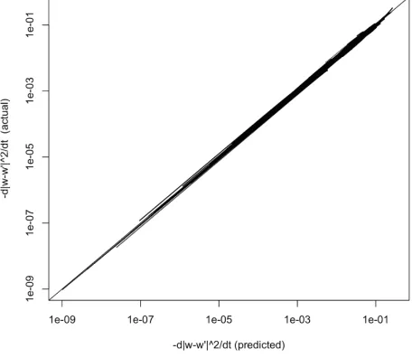
nor-mal distribution (mean 0, s.d. 1). Then, for each of those 10,000 simulations, a perturbed mate was made by adding normally distributed noise (mean zero, s.d. 0.1) to w(0)to get w0(0). The second-order Taylor approximation to Daround γ = 0 is D ≈(1/2)γTHγ, whereγ = CT(w0 −w). This
[image:6.612.313.541.431.629.2]was used to predict D on each of the 300 update steps for each pair. Results, shown in Figure 2, ver-ify the accuracy of the approximation (and hence corroborate the analysis), and show that D was in every case negative, i.e., that each learner consis-tently converged with its mate over time.
Figure 2: Actual vs. predicted rate of convergence between pairs in weight space. Values have been multiplied by -1 so that logarithmic axes can be used. Each streak is one ofN= 1000
pairs (9,000 more omitted to reduce image size).
6 Similar initial weights imply similar 2AFC learning curves
performance in a learner that starts at0 never im-proves faster than it did att= 0(Proposition 2). Just
how closely is the 2AFC learning curve of the near-0learner tethered to the bounded learning curve of the at-0learner?
Proposition 4. For any w and w0, the difference
∆λ(w,w0) = Ew0[λ+,−]−Ew[λ+,−]is bounded
by|∆λ| ≤ kw0 −wk√mcrange, wherecrangeis the
largest absolute difference between any two entries inC.
Proof. From Equation 14, the difference between the two learners in the expected log-odds of a cor-rect test response is given by∆λ(w,w0) = (w0− w)TC(r+ −r−). By Cauchy-Schwarz, this is no
greater thankw0 −wkkC(r+−r−)k. Each entry inC(r+−r−)is the difference between the average
scores of the positive versus negative test stimuli on one of the constraints, which is at mostcrange. Thus
kC(r+−r−)k ≤√mcrange.
Since kw0(t) − w(t)k ≤ kw0(0)− w(0)k by Proposition 3, the 2AFC learning curve of a learner that started atw0(0) 6= 0 cannot stray further than
kw0(0)k√mcrangefrom one that started at0. In actual practice, the experimenter will often di-vide the candidates into positive and negative test sets in a controlled way, so that the two sets receive, on average, the same score from all but some small numberm?of themconstraints, which we can
sup-pose are Constraintsc1 throughcm?. Since theith
entry of C(r+−r−) is the average difference
be-tween the positive and the negative test sets in their score on theith constraint, all but the firstm?of the entries will be as close to zero as the experimenter is able to arrange. In that case, we can truncatew,w0, andCto their firstm?entries or rows, tightening the bound to|∆λ| ≤ kw0?−w?k√m?c?
range.
Proposition 5. LetM = maxikCi,·k be the norm of the row ofC with the largest norm, and letR = maxi|Ci,·1|be the largest absolute row sum inC.
Then the difference between the initial rate of 2AFC improvement of a learner that starts atw= 0 and one that starts atw0 near0is bounded by
|d∆λ/dt|w=0≤ kw0k
M2
n +
R2 n2
m√m?crange (32)
Proof. Use Equation 19, approximating p0 −p ≈ JCT(w0−w), whereJ
i,j=∂pi/∂γjis the Jacobian ofp0as a function ofγ. From Equation 27 it follows
thatJ =diag(p)−ppT (i.e.,J =−H/4; see Eqn.
31). Then
|d∆λ/dt| ≈(w0−w)TCJCTC(r+−r−) ≤ k(w0−w)TkkCJCTkkC(r+−r−)k
(33)
wherek · k, for matrices, is the operator norm, the
maximum factor by which the matrix can stretch a vector (Strang, 1980, 284). Since CJCT is
symmetric, its operator norm is simply its largest eigenvalue, which is no larger than ma, where
a= maxi,j|(CJCT)i,j|(Zhan, 2006, Corollary 2). What isa?
For w = 0, we have J = n1I − n1211T, so
CJCT = 1nCCT − 1
n2C11TCT. Then
1 n(CC
T) i,j
=
1
n|Ci,··Cj,·|
≤1
nmaxi |Ci,··Ci,·|
≤1 nM
2
(34)
Likewise,
1 n2C11
TCT
≤
1
n2 maxi,j |(C1)i·(C1)j|
≤ 1
n2 maxi(C1) 2
i
≤n12R2
(35)
Hence
a= max
i,j |(CJC T)
i,j| ≤ 1
nM
2+ 1
n2R
2 (36)
and so, sincekCJCTk ≤ma,
kCJCTk ≤m
1 nM
2+ 1
n2R 2
(37)
A row ofCcorresponds to a constraint, each
en-try being the score that that constraint gives to one candidate. Since all of those scores are less thancmax (the largest absolute value of any element inC), we
haveM2 ≤nc2
maxandR2 ≤(ncmax)2. Hence
|d∆λ/dt|w=0≤ kw0km
√ m?c2
maxcrange (38)
This is a worst-case estimate, based on very weak hypotheses about C and on the blunt
instru-ment of the vector and matrix norms, which ig-nore exploitable structure. Stronger hypotheses per-mit improvment. For example, suppose C is
bi-nary, and let di = n1C1 be the proportion of 1’s in Row i. Each entry (CCT)i,j is the number of 1’s that appear in the same column in Rows i and j, and hence is at most the smaller of the two row
sums, so 1
n(CCT)i,j ≤ min{di, dj}. Each entry
(C11TCT)
i,j is the product of the row sums of Rows i and j, so n12(C11TCT)i,j = didj.
Con-sequently,
a= max
i,j |(CJC T)
i,j| ≤min{di, dj} −didj
≤min{di(1−dj), dj(1−di)}
≤1/4
(39)
To justify this last step, suppose without loss of generality that di(1 − dj) ≤ dj(1 − di). Then
a2 = (di(1−dj))2 ≤ di(1−dj)dj(1−di) =
di(1−di)dj(1−dj) ≤ (1/4)(1/4), so unsquaring on both sides yieldsa≤1/4. It follows that
|d∆λ/dt|w=0 ≤ kw0k
1 4m
√
m? (40)
Suppose further that the entries ofCare modelled
as i.i.d. Bernoulli trials with Pr(Ci,j = 1) = s. ThenM2 = max
iPnj=1Ci,j2 =
Pn
j=1|Ci,j| = R. Ifnis large, the row sums are approximately
sam-ples from a normal distribution with mean ns and
standard deviationpns(1−s). The expected value
of the maximum of a sample of sizemfrom the
stan-dard normal distribution N(0,1) is approximately √
2 logm (Cram´er, 1946, 374). Hence E[M2] =
E[R] = (ns+pns(1−s)2 logm). Asn → ∞,
E[M2]/n → s, whileE[R2]/n2 = (E[R]/n)2 =
(E[M2]/n)2 → s2. Thus k(CJCT)k → (s+ s2)m=s(1 +s)m, andc
max=crange= 1, so from Equation 40, we have
E[|d∆λ/dt|w=0]≤ kw0km
√
m?min
1
4, s(1 +s)
(41) Equation 41 was checked against 10,000 simu-lations, generated as described in Section 4. The yoked pairs consisted of one learner that started at w(0) =0, and one that started atw0(0)with entries
sampled from a normal distribution with mean 0 and standard deviation 0.1. In calculating the bound,m? was set equal to m. The actual value was always
less than the bound, with the minimum difference being 0.01405. The bound was usually a substantial overestimate, the median difference being 5.372 and the maximum 30.51. In the subset where the near-zero learner’s initial performance was near chance (|λ0(0)| ≤ 1/10) and initial improvement was near
zero (|dλ0/dt| ≤ 1/10), a total of 1075 cases, the
bound proved much tighter, overestimating by a me-dian of 0.591 and a maximum of 0.998. These cases tended to have either smallmor extremes.
7 Putting the bounds together
One way that these bounds might be applied in practice is as follows. Suppose we hypothesize that the learner’s initial weightsw0(0)are such that kw0(0)k ≤ w, and we experimentally measure ini-tial performance to beλ0(0) = 0and the initial
im-provment rate to bedλ0/dt(0) = 0. Proposition 5
then gives us a bound — call itb — on the initial improvement rate for an otherwise identical learner withw(0) = 0. By Proposition 2, the slope of the hypothetical0-learner’s 2AFC curveλ(t)never ex-ceedsb. That curve would have started atλ(0) = 0,
sincew(0) = 0 makes all candidates equally har-monic. Hence the hypothetical 0-learner’s 2AFC curve is bounded byλ(t) ≤ bt. By Proposition 3,
the observed and hypothetical learner converge in weight space, which by Proposition 4 means that
λ0(t)≤bt+w√m?crange. Conversely, ifλ0(t)ever
exceeds this value, we know that w0(0)must have
been more thanw, contrary to hypothesis.5
5We also have to assume that the experiment has sufficient
8 When initial weights are far from zero, 2AFC performance can accelerate
If the initial weights are far from 0, then even a simple constraint set can yield abrupt learning. For
n = 4, let C = I4, the identity matrix of order
4 (i.e., 4 candidates, 4 constraints, each constraint gives a 1 to just one candidate). If we setw(0) = (x,−x,0,0)T, p+ = r+ = (1/2,1/2,0,0)T, and
r− = (0,0,1/2,1/2)T, the 2AFC curve starts out
flat at 0 and stays that way (longer the biggerxis),
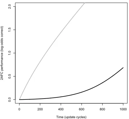
[image:9.612.73.288.336.534.2]then starts climbing rapidly as shown in the black curve on Figure 3.
Figure 3: 2AFC learning curves forn = 4, C = I4, and
w0 = (6,−6,0,0)T (black curve) or(6,−6,6,−6)T (gray
curve), with p+ = r+ = (1/2,1/2,0,0)T, and r− =
(0,0,1/2,1/2)T. Other parameters:η= 1/100.
0 200 400 600 800 1000
0.0
0.5
1.0
1.5
2.0
Time (update cycles)
2AF
C
p
erf
orma
nce
(l
og
-o
dd
s
co
rre
ct
)
The idea behind this construction is that initially, every negative candidate is much less probable than half of the positive candidates, and much more prob-able than the other half, so that the outcome of a 2AFC trial is 50% likely to be correct (0 logits). The learner then spends ages laboriously hauling up the low-frequency half of the positive candidates, and letting down the negative candidates, until the low-frequency positive candidates finally start winning a
brief but huge improvment rate that would satisfy the hypoth-esis of Proposition 2 and thus allow later unexpected sudden improvement.
noticeable number of 2AFC competitions. The con-struction can be carried out for anyCthat makes it
possible to sandwich the initial probabilities of the positive (negative) candidate between those of the negative (positive) ones by artful choice ofw(0).
9 Discussion
Since abrupt learning has been observed in human phonological acquisition in nature Smith (1973); Macken and Barton (1978); Vihman and Velleman (1989); Barlow and Dinnsen (1998); Levelt and van Oostendorp (2007); Gerlach (2010); Guy (2014) and in the lab Moreton and Pertsova (2016), the question of when a gradual learning ruletranslates into gradual learningperformanceis pertinent. For the learner and experimental paradigm studied here, transfer from UG or from previous learning is a nec-essary condition for abruptness. This result spawns many further questions, among them:
The non-abrupt gray curve in Figure 3 shows that not just any set of large non-zero initial weights, paired with just any training and test distribution, leads to abrupt learning in the model. Which ones do? What are the most general sufficient conditions? Phonological theory offers many proposals about the initial state of L1 or L2 learning (e.g., Demuth (1995); Gnanadesikan (1995); Smolensky (1996); Pater (1997); Broselow et al. (1998); Boersma and Levelt (2000); Curtin and Zuraw (2002); Hayes (2004); Wilson (2006); Hayes et al. (2009); Jesney and Tessier (2011); White (2014)); what predictions follow for abruptness?
In human learners, is abrupt learning associated with transfer of constraint weights from UG, L1, or previous training in the lab? What is going on during apparent initial stagnation? Does it actually consist of steadyunlearning of a pre-existing grammar?
References
Agresti, A. (1990). Categorical data analysis. New York: Wiley Interscience.
Ashby, F. G., L. A. Alfonso-Reese, A. U. Turken, and E. M. Waldron (1998). A neuropsychological theory of multiple systems in category learning. Psychological Review 105(3), 442–481.
Barlow, J. A. and D. A. Dinnsen (1998). Asymmet-rical cluster development in a disordered system. Language Acquisition 7(1), 1–49.
Berger, A. L., S. A. Della Pietra, and V. J. Della Pietra (1996). A maximum entropy approach to natural language processing. Computational Lin-guistics 22(1), 39–71.
Boersma, P. (1998).Functional Phonology: formal-izing the interactions between articulatory and perceptual drives. Ph. D. thesis, University of Amsterdam.
Boersma, P. and B. Hayes (2001). Empirical tests of the Gradual Learning Algorithm. Linguistic In-quiry 32, 45–86.
Boersma, P. and C. Levelt (2000). Gradual
constraint-ranking learning algorithm predicts ac-quisition order. In Proceedings of Child Lan-guage Research Forum 30, Stanford, California, pp. 229–237.
Boersma, P. and J. Pater (2016). Convergence prop-erties of a gradual learning algorithm for Har-monic Grammar. In J. J. McCarthy and J. Pater (Eds.),Harmonic Grammar and Harmonic Seri-alism, pp. 389–434. Sheffield, England: Equinox. Boyd, S. and L. Vandenberghe (1999).Convex
opti-mization. Cambridge University Press.
Broselow, E., S.-I. Chen, and C. Wang (1998). The emergence of the unmarked in second language phonology. Studies in Second Language Acquisi-tion 20, 261–280.
Cram´er, H. (1946). Mathematical methods of statis-tics. Princeton, New Jersey: Princeton University Press.
Curtin, S. and K. R. Zuraw (2002). Explaining constraint demotion in a developing system. In B. Skerabela, S. Fish, and A. H.-J. Do (Eds.), Papers from the 26th Boston University Confer-ence on Language Development (BUCLD 26), Somerville, pp. 118–129. Cascadilla Press. Demuth, K. (1995). Markedness and the
develop-ment of prosodic structure. In J. Beckman (Ed.), Proceedings of the 25th Meeting of the North-East Linguistics Society, Amherst, Mass., pp. 13–26. Graduate Linguistics Students Association. Elman, J. L., E. A. Bates, M. H. Johnson,
A. Karmiloff-Smith, D. Parisi, and K. Plunkett (1996). Rethinking innateness. Cambridge, Mas-sachusetts: MIT Press.
Fischer, M. (2005). A Robbins-Monro type learn-ing algorithm for an entropy maximizlearn-ing version of Stochastic Optimality Theory. Master’s thesis, Humboldt-Universit¨at, Berlin.
Gerlach, S. R. (2010). The acquisition of conso-nant feature sequences: harmony, metathesis, and deletion patterns in phonological development. Ph. D. thesis, University of Minnesota.
Gnanadesikan, A. (1995, October). Markedness and faithfulness constraints in child phonology. Manuscript # 67, Rutgers Optimality Archive
(roa.rutgers.edu).
Goldwater, S. J. and M. Johnson (2003). Learning OT constraint rankings using a maximum entropy model. In J. Spenader, A. Erkisson, and O. Dahl (Eds.), Proceedings of the Stockholm Workshop on Variation within Optimality Theory, pp. 111– 120.
Guy, G. R. (2014). Linking usage and grammar: generative phonology, exemplar theory, and vari-able rules. Lingua 142, 57–65.
Hayes, B. (2004). Phonological acquisition in Op-timality Theory: the early stages. In R. Kager, J. Pater, and W. Zonneveld (Eds.), Constraints in phonological acquisition, Chapter 5, pp. 158– 203. Cambridge, England: Cambridge University Press.
Hayes, B. and C. Wilson (2008). A Maximum Entropy model of phonotactics and phonotactic learning. Linguistic Inquiry 39(3), 379–440. Hayes, B., K. Zuraw, P. Sipt´ar, and Z. Londe (2009).
Natural and unnatural constraints in Hungarian vowel harmony. Language 85(4), 822–863. Horn, R. A. and C. R. Johnson (1985).Matrix
anal-ysis. Cambridge, England: Cambridge University Press.
J¨ager, G. (2007). Maximum Entropy models and Stochastic Optimality Theory. In J. Grimshaw, J. Maling, C. Manning, J. Simpson, and A. Zae-nen (Eds.),Architectures, rules, and preferences: a festschrift for Joan Bresnan, pp. 467–479. Stan-ford, California: CSLI Publications.
Jarosz, G. (2016). Learning with violable con-straints. To appear in: Jeff Lidz, William Snyder, and Joe Pater (eds.),The Oxford handbook of de-velopmental linguistics. Oxford, England: Oxford University Press.
Jesney, K. (2016). On the relationship between learning sequence and rate of acquisition. In G. la-fur Hansson, A. Farris-Trimble, K. McMullin, and D. Pulleyblank (Eds.),Proceedings of the An-nual Meeting on Phonology 2015, Volume 3. Lin-guistic Society of America.
Jesney, K. and A.-M. Tessier (2011). Biases in Har-monic Grammar: the road to restrictive learning. Natural Language and Linguistic Theory 29(1), 251–290.
Johnson, M. (2007, November). A gentle in-troduction to Maximum Entropy models and their friends. Slides from a talk,
ac-cessed at web.science.mq.edu.au/
∼mjohnson/ papers/CompPhon07-slides.pdf
on 2013 August 6.
Kurtz, K. J., K. R. Levering, R. D. Stanton, J. Romero, and S. N. Morris (2013). Human learning of elemental category structures: revis-ing the classic result of Shepard, Hovland, and Jenkins (1961).Journal of Experimental Psychol-ogy: Learning, Memory, and Cognition 39(2), 552–572.
Levelt, C. and M. van Oostendorp (2007). Feature co-occurrence constraints in L1 acquisition. Lin-guistics in the Netherlands 24(1), 162–172. Love, B. C. (2002). Comparing supervised and
un-supervised category learning. Psychonomic Bul-letin and Review 9(4), 829–835.
Luce, R. D. (2005 [1959]).Individual choice behav-ior: a theoretical analysis. New York: Dover. Macken, M. A. and D. Barton (1978, March). The
acquisition of the voicing contrast in English: a study of voice-onset time in word-initial stop con-sonants. Report from the Stanford Child Phonol-ogy Project.
Maddox, W. T. and F. G. Ashby (2004). Dissociating
explicit and procedural-learning based systems of perceptual category learning. Behavioural Pro-cesses 66, 309–332.
Moreton, E., J. Pater, and K. Pertsova (2017). Phonological concept learning. Cognitive Sci-ence 41(1), 4–69.
Moreton, E. and K. Pertsova (2016). Implicit and explicit processes in phonotactic learning. In TBA (Ed.),Proceedings of the 40th Boston Uni-versity Conference on Language Development, Somerville, Mass., pp. TBA. Cascadilla.
Pater, J. (1997). Minimal violation in phonological development. Language Acquisition 6(3), 201– 253.
Pater, J. (2008). Gradual learning and convergence. Linguistic Inquiry 39(2), 334–345.
Pater, J. (2016). Universal Grammar with weighted constraints. To appear in: John McCarthy and Joe Pater (eds.), Harmonic Grammar and Harmonic Serialism.
Pater, J. and E. Moreton (2012). Structurally bi-ased phonology: complexity in learning and ty-pology. Journal of the English and Foreign Lan-guages University, Hyderabad 3(2), 1–44. Smith, J. D., M. E. Berg, R. G. Cook, M. S. Murphy,
M. J. Crossley, J. Boomer, B. Spiering, M. J. Be-ran, B. A. Church, F. G. Ashby, and R. C. Grace (2012). Implicit and explicit categorization: a tale of four species. Neuroscience and Biobehavioral Reviews 36(10), 2355–2369.
Smith, N. (1973). The acquisition of phonology: a case study. Cambridge, England: Cambridge University Press.
Smolensky, P. (1996). On the
comprehen-sion/production dilemma in child language. Lin-guistic Inquiry 27, 720–731.
Strang, G. (1980). Linear algebra and its applica-tions. Orlando, Florida: Academic Press.
Vihman, M. M. and S. Velleman (1989). Phonolog-ical reorganization: a case study. Language and Speech 32, 149–170.
White, J. (2014). Evidence for a learning bias against saltatory phonological alternations. Cog-nition 130, 96–115.